Article

The Comparison of Density-Based Clustering Approach among Different Machine Learning Models on Paddy Rice Image Classification of Multispectral and Hyperspectral Image Data

1
Information Technology, Ling Tung University, Taichung 40851, Taiwan
2
Department of Soil and Environmental Sciences, National Chung Hsing University, Taichung 40851, Taiwan
*
Author to whom correspondence should be addressed.
Agriculture 2020, 10(10), 465; https://doi.org/10.3390/agriculture10100465
Submission received: 29 August 2020 / Revised: 1 October 2020 / Accepted: 5 October 2020 / Published: 10 October 2020

Abstract

:
The analysis, measurement, and computation of remote sensing images often require enhanced unsupervised/supervised classification approaches. The goal of this study is to have a better understanding of (a) the classification performance of multispectral image and hyperspectral image data; (b) the classification performance of unsupervised and supervised models; and (c) the classification performance of feature selection among different models. More specifically, the multispectral images and hyperspectral images with high spatial resolution are well accepted for improving land use and classification. Hence, this study used multispectral images (WorldView-2) and hyperspectral images (CASI-1500) and focused on the classifiers K-means, density-based spatial clustering of applications with noise (DBSCAN), linear discriminant analysis (LDA), and back-propagation neural network (BPN). Then the feature selection (principle component analysis, PCA) on four classifiers is studied. The results show that the image material of CASI-1500 classification accuracy is slightly better than that of WorldView-2. The overall classification of BPN is the best, the overall data has a κ value of 0.89 and the overall accuracy is 97%. The DBSCAN presents a reality with good accuracy and the integrity of the thematic map. The DBSCAN can attain an accuracy of about 88% and save 95.1% of computational time.

1. Introduction

Rice is an important crop in Taiwan, therefore, the Agriculture and Food Agency Council of Agriculture Executive Yuan in Taiwan has focused on the location and spatial distribution of paddy rice planting area. The rice spatial information database is used by the Taiwan Food Bureau to grasp the changes in rice production through field surveys and remote sensing image analysis. The use of remote sensing detection technology is to classify the use or growth of agricultural land. It can estimate the planting area or crop yield which has become an acceptable method. In Taiwan, there have been studies using remote sensing images to establish rice yield estimation models [1] and to quantify the long-term average yield and spatial distribution of rice [2,3].
Excessive studies on remote sensing image classification are contributed by experts and scholars for generating those thematic maps [3,4,5,6,7]. They proposed different image classification models through supervised or unsupervised classification methods [8,9,10] and considered computing them with different algorithms. The target categories on how to improve classification accuracy have been extensively discussed. These arise two basic reasons for material image data [4] and approaches which make the interpretation interesting and different:
  • The ability to interpret different types of characteristic spectra is solved by increasing ancillary information [5,6,7,11,12] to improve the classification accuracy of an image. Researchers usually use supervised classifiers to resolve image processing problems [10,13,14,15]. Therefore, ancillary information has become an alternative component of the analyzed dataset to enhance classification outcomes. Adding different types of band information may help improve classification results.
  • Suitable classification approaches for models can improve classification results. In addition, the selection of applicable mathematical algorithms for high-precision parameters is important to model the data and verify the classification outcomes. Generally speaking, the establishment of synchronized image capture and ground survey operations can provide high accuracy in various modeling and different features [14,15,16,17,18,19].
In Taiwan, aerial orthophotos and satellite images are often used to study the use of classified agricultural land. (1) The aerial orthophotos data of Taiwan has a spatial resolution of 25 cm. In the past, this kind of datum is difficult to obtain. Unfortunately, the images are only red, green, and blue visible spectral bands, with a lack of near-infrared band information. Because the visible spectral values are similar, the classification of the green crops effect is quite limited. Leaf pigments and cell walls are hardly absorbed in the near-infrared region (700–1300 nm). The reflectance spectrum of the leaves is quite different in the near infrared region. In a peak area, the reflectivity is related to various factors such as the thickness, size, arrangement, and cell contents of mesophyll cells. (2) The spatial resolution of the satellite image is too rough. The small area of farmland cannot be distinguished. The length of the farmland is located between 10 and 50 m and the width is generally 7 to 20 m. Therefore, the spatial resolution of 6 to 40 m satellite image data in the target area of Taiwan is very hard to use. In other words, the spatial resolution is too low to separate various agricultural land uses. Part of the research will collect images from multiple periods and increase the accuracy of classification by adding time-series information [2,6]. Therefore, the multispectral image and/or hyperspectral image with high spatial resolution and multiple bands are the research materials that domestic scholars would like to obtain. At present, many studies have used high-resolution with multispectral WorldView series of image data. This was combined with deep learning for research and analysis, and the classification results were quite good [20,21,22]. Hyperspectral images have a finer and continuous spectrum, the number of bands is 10–20 times higher than that of the multispectral data, and the resolution is enhanced by a small wavelength which is conducive to the segmentation and extraction of fine information. Therefore, hyperspectral images are often used as materials to develop estimation models or algorithms for quantifying targets [23,24,25].
In 2014, the Taiwan Agriculture Committee launched the “Golden Corridor Agriculture New Plan and Action Plan” and entrusted the Executive Institute of Agricultural Experiments to collect land use information for the second crop of the Golden Corridor in 2014. The study used multispectral image and hyperspectral image data combined with field investigation to establish an accurate agricultural classification method through image data. Our analytical data and the field survey data in this study are the sample data provided by the research institute, Taiwan Agricultural Research Institute, Council of Agriculture (TARI). Due to a lack of appropriate classification algorithms for machine learning, the selection of suitable mathematical algorithms is required to test and conduct high-precision parameter screening modeling and verification of various studies.
This set of data of TARI is a very rare research material. They also involved the increase in band information and resolution or high spatial dimension. The database is relatively large and requires a good classification method for investigation and research. Clustering can be done well by selecting an appropriate algorithm. This can aggregate similar data into corresponding clusters. Unfortunately, it encounters some problems by applying them. In most cases, it seems difficult to recognize which input parameter plays an important role for a particular target. If the user lacks domain knowledge, the survey data must be re-evaluated. Therefore, most of the studies point out that the accuracy of supervised classification is higher than that of unsupervised classification. However, considering the research area of general telemetry images, there may not be ground true data that can be used directly. The training and testing data of land classification require a lot of manpower and resources to produce them for a supervised model. In other words, the land use of in situ surveys is very time-consuming work. Moreover, the image could be also influenced by weather factors. On the other hand, delay in image acquisition time will also produce a slight inconsistency during image capture. This all may result in a slight inaccuracy for final classification results. Land classification will increase the problem of land-use change, such as short-term crop conversion, which increases the difficulties in image classification. Therefore, it was decided to use two widely used unsupervised classification methods: K-means and density-based spatial clustering of applications with noise (DBSCAN). On the other hand, it also used two supervised classification methods with higher classification accuracy: linear discriminant analysis (LDA) and Artificial Neural Network (ANN)–backpropagation neural network (BPN). In this study, the classification accuracy was compared and thematic maps were drawn.
K-means has been developed by many software or toolboxes. It is easy to take and apply which is also the most common unsupervised classification model. DBSCAN which provides an interesting solution for image classification. This data analysis can be performed in an in situ process which does not request previously investigating the rice and non-rice zone. Linear discriminant analysis (LDA) is a well known approach with some labeled data which is selected as the parallel study. The LDA classification was by Blei et al. [26], who suggested that the simplicity and effectiveness of the model, the trend of the topic model research, has been set. At present, several neural network models have been proposed and they have been successfully used in business forecasting and engineering applications. Vellido et al. [27] collected the commercial analysis of the use of neural networks from 1992 to 1998. There are approximately 78% of applications using supervised backpropagation neural network (BPN) as an analytical model. Gupta and Stafford [28] also suggested that BPN is suitable for solving problems in prediction, classification, and system model construction. It is widely used in the natural and social sciences [13,14,15].
The purpose of this study was to use the multispectral and hyperspectral images. This study was also designed to compare the difference between the unsupervised classification models and supervised classification models. The ground truth data, combined with common mathematical algorithms such as K-means, DBSCAN, LDA, and BPN are applied for rice area classification. It is decided to examine and compare the classification accuracy of paddy rice and to apply the classification algorithm in decision making. The research further presents the classification results then discusses the reasons that may lead to poor classification results.

2. Materials and Methods
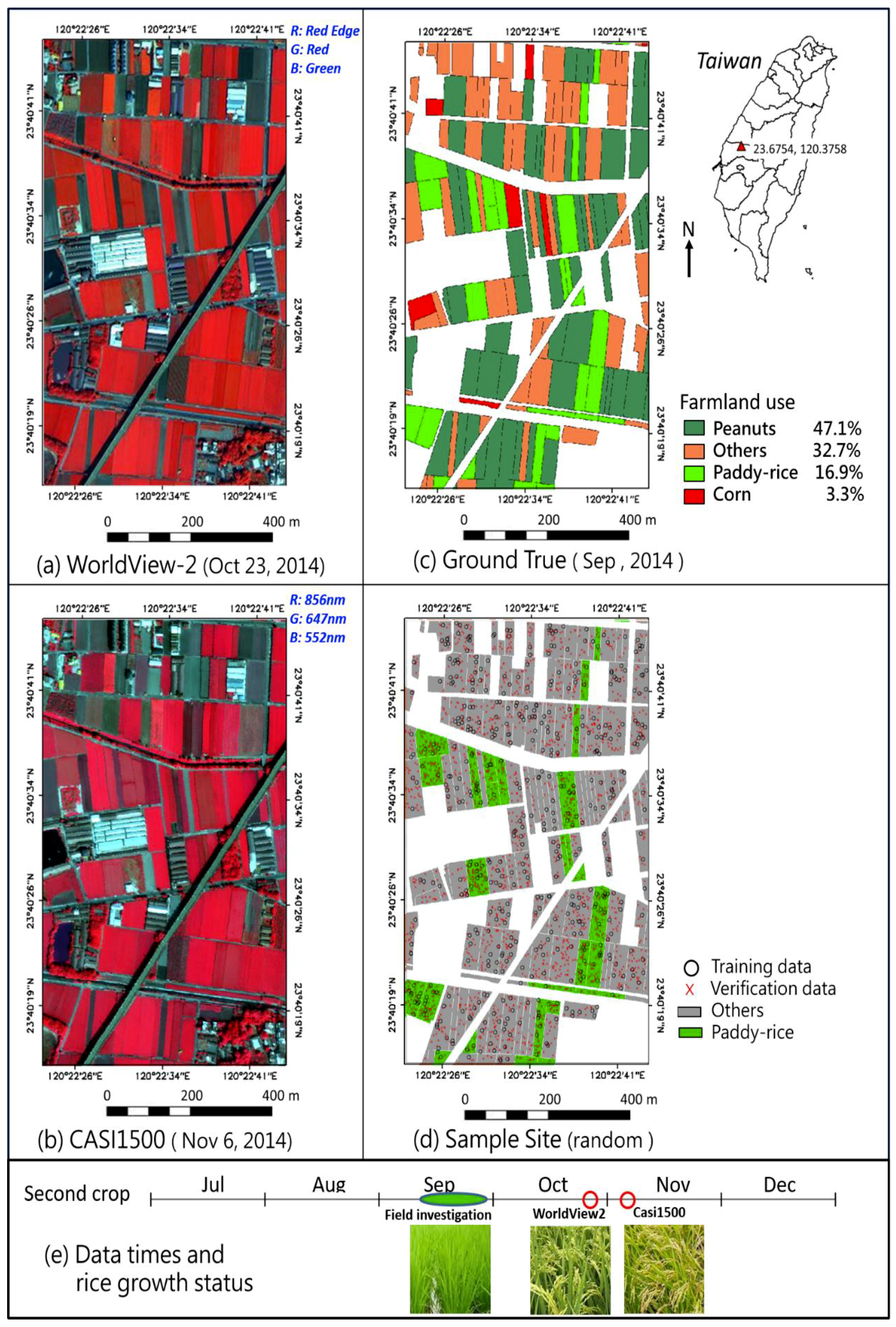
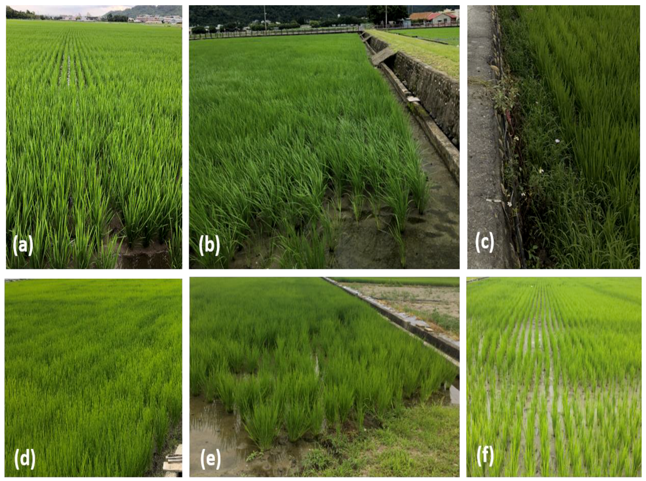
2.1. Study Area

The Golden Corridor located in Yunlin County is the sample data provided by the research institute, TARI. The longitude and latitude of the Golden Corridor address is at 23.6754° N and 120.3758° E, respectively, with a high-rail speed track across. The study area has a length of the test area of 942 m and a width of 569 m with the size of the area of 0.536 km2. This study used multispectral image (WorldView-2) and the hyperspectral image (CASI-1500) to establish an accurate agricultural land interpretation method through image classification. In the second season crop, a large number of paddy fields are converted into corn, cabbage, groundnut, etc. The utilization is 15% for paddy fields and 60% for dry fields. Figure 1a,b show the location of the test area and the false color image of the WorldView-2 image and CASI-1500. The land use survey was conducted during September 2014. The ground truth state is shown in Figure 1c. The utilization is 47.1% for peanuts, 32.7% for others, 16.9% for paddy rice, and 3.3% for corn. Figure 1d shows the spatial distribution of 500 training data (generated by random numbers) used for the supervised classification and 2000 verification data (generated by random numbers) for comparing the classification accuracy. Figure 1e shows the rice growth period corresponding to the data collection time. The second-stage crop is mainly planted at the end of July and harvested in mid-November. Due to the large time difference between the field survey and image obtained, some crops were harvested.

2.2. Introduction on CASI-1500 and WorldView-2 Image Data

Sample image data were provided by TARI. TARI purchased the multispectral images of the test area from the manufacturer. Table 1 lists the full width at half maximum (FWHM) of each band of multispectral and the hyperspectral data. The hyperspectral image was commissioned and used the CASI-1500 sensor to capture images with image wavelengths ranging from 350 to 1050 nm, 72 bands, and a spatial resolution of 1 m. The CASI-1500 shooting date was on 6 November 2014. The image has been processed completely by TARI for radiation correction, space correction, and atmospheric correction. The multispectral image WorldView-2 was commissioned by DigitalGlobe. The image was taken on 23 October 2014. WorldView-2 have eight bands (List in Table 1), a spatial resolution of 2 m. We resampled the 2 m spatial resolution of the Worldview-2 image to 1 m, so that the data have the same spatial position for comparison. Worldview-2 data were calibrated by a TARI. Due to poor weather, the video shooting took place more than the field investigation did one month late. The state of rice shows the maturity levels of different growth (Figure 1e), while when the WorldView-2 image took place, the rice spike was mainly green. In the CASI-1500 image, the local rice spike has turned yellow. Thus, the difference in the band information between different patches may exist. However, the classifiers in this study can compare the classification diversity for the CASI-1500 image data.

2.3. Selection of Training and Testing Samples

As mentioned previously, due to the small test area and the difficulty in obtaining data, it was decided to select training samples and testing samples from the same figure with random selection of pixel in each kind of the corps. The study selected 500 samples (100 paddy rice, 400 others) as the modeling parameters in the farmland area (about 0.15% of the data), and it was based on the random number method. There were 2000 samples (600 paddy rice, 1400 others) selected for testing the data of model verification. In addition, the test applied the classification model to the entire region and further compared the classification accuracy of various algorithms. The data distribution is shown in Figure 1d.

2.4. Classification Modeling for Experiments

To have a better understanding of the classification performance of K-means, DBSCAN, LDA, and BPN, this study was designed to construct parallel approaches on a given rice field to observe the discrepancy of classification outcomes. Due to the large number of image bands in the study, the study will use PCA for feature selection, and compare to which accuracy it was improved. Principal component analysis (PCA) is a well known multivariate approach to reduce the data dimensions for data mining. In the initial stage, the usage of PCA considers a smaller number of variables in a multivariate dataset. Mathematically, PCA is a process that decomposes the covariance matrix of a matrix into two parts: eigenvalues and column eigenvectors. In the second stage, the reduction process is achieved by taking p variables X1, X2, …, Xp and combining them to produce principal components (PCs) PC1, PC2, …, PCp, which are uncorrelated. These PCs are also termed eigenvectors. Then, the lack of correlation is a useful property as it means that the PCs are measuring for new “dimensions” in the data. However, the new calculated PCs are ordered. For instance, the PC1 exhibits the largest amount of variation, PC2 exhibits the second largest amount of variation …… and so on. When using PCA, it is hoped that the eigenvalues of most of the PCs will be low so that they are virtually ignorable. Consequently, it sieves a small amount of variables in the original number of variables (X variables) which can be described using the smaller number of PCs [29,30]. The classifiers are K-means, DBSCAN, LDA, and BPN. Then, the PCA is used for dimension selection. We set 65% as the largest eigenvalue of the WorldView-2 (eight bands by PCA selection for five PCAs) and CASI-1500 (72 bands by PCA selection for 46 PCAs) to compare with a study example to determine whether the influenced factor works better or not.

2.4.1. K-Means

K-means is an iterative clustering algorithm by MacQueen [31]. The items are moved among a set of clusters until the desired set is reached. The cluster center is determined as the mean value of each cluster. While it implements the K-means approach, the first step is to assign numbers of clusters and the initial value for each cluster center. Then, it assigns each item ti to the cluster, which has the closest center, and to calculate the new mean value for each cluster as a new center. These steps were repeated until the convergence criteria were successfully met. This algorithm is inherently iterative to approach the optimal solution. Hence, the performance of the K-means will depend on the initial positions of the cluster center which makes it advisable to either employ a proper initial cluster set or allow more iterations.

2.4.2. DBSCAN

The density-based clustering (DBSCAN) approach [32,33,34,35,36] resolved this type of problem. The clusters are allocated in the dense regions in the data space which separates the lower density of points by regions. The DBSCAN algorithm is based on this intuitive notion of “clusters” and “noise”. The key idea is that for each point of a cluster, the neighborhood of a given radius has to contain at least a minimum number of points. The DBSCAN algorithm applies a set of points in a given space as well as aggregates data points which are packed together nearby (points with many nearby neighbors). It can also treat as outlier points (noise) that allocate alone in low-density regions. In addition, spatial datasets using DBSCAN can handle huge amounts of data with smaller related cluster patterns in various dimensions. This process can decrease a huge amount of computation time. The shapes of the image data clusters should be adjusted for bad cases which are always favorable and should be or extracted. DBSCAN employs a data clustering algorithm that considers a density-based clustering process by evaluating the data distribution and location. A set of points in some space were grouped together with the concept of density. As the algorithm was applied, it closely aggregated nearby sample points. It also marked as outlier points those that were alone in low-density regions (whose nearest neighbors were too far away). DBSCAN is one of the most common clustering algorithms used for handling improperly distributed sample data, especially in Geosciences or image classification. Most of the readers are not familiar with DBSCAN, thus, a brief introduction to DBSCAN follows.
First, assume a set of points is to be clustered. A developed computer program by Python follows the DBSCAN algorithm. The definition of the core points, reachable points, and outliers are introduced as follows. A core point (P) is selected by the computer program if at least MinPts nearby points are within distance ε of it (including p). Those points are defined as directly reachable from p. The program will check (a) that none of the points are directly reachable from a non-core point; and (b) that each of the points is directly reachable from a core point. The program will also check that each point q is reachable from p if there is a series of path p1, ..., pn. Considering one of the points p1 = p and pn = q, for each pi + 1, find all the points that are directly reachable from pi and record these points into a matrix. The program defines those points that are not reachable from any other point as outliers. More specifically, if p is selected as a core point, then it is selected as a cluster aggregated with the corresponding nearby points that may be reachable from it. Those corresponding nearby points may be core or non-core points. The developed program will also check that each computed cluster includes at least one core point. The non-core points can be part of a cluster, and the program will not use them to reach more points. The DBSCAN process is illustrated as follows. The Eps is defined as all the points corresponding to region O with the given associated radius. Please see Figure 2a. The user should determine the minimal number of data point p with regard to the clustering set P. Please see Figure 2a. The DBSCAN clustering process is as follows.
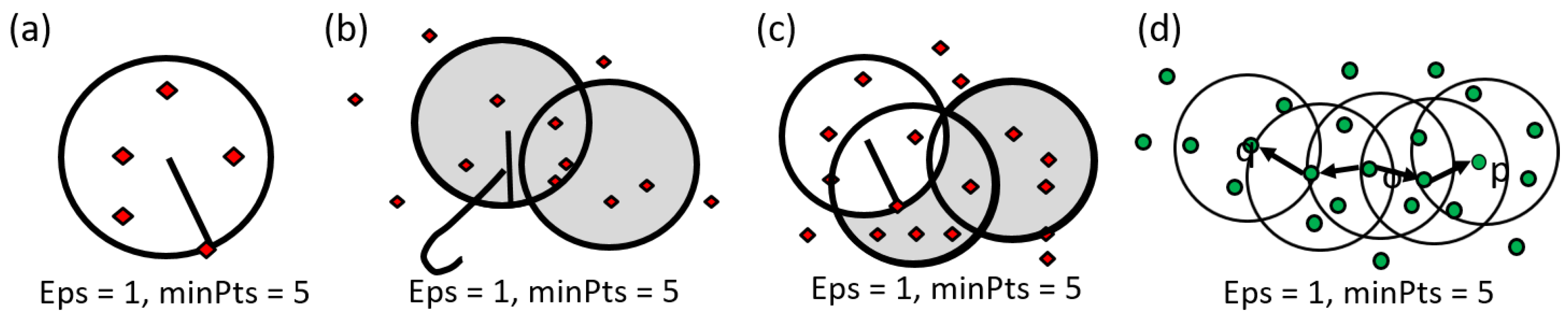
  • Directly density reachable: each of the sample points is tested against the cluster-center with the associated radius. If this point falls in the range, the rest of the points will also be tested. This procedure is called directly density reachable which makes a cluster group of D. Please see Figure 2b. The developed program system will automatically count the number of sample data, which is either greater than the minimum data number given or not. This minimal data number given is named as MinPts. Please see Figure 2c. For instance, if the user defined it as MinPts = 5, the program will search the nearby data which fall in this range with the Eps = 1.
  • Density reachable: in certain cases, for instance, the data points in a scatter diagram are a group but they are distributed linearly. The program will check each of the data with each of their neighboring points to see whether they falls in the minimal density or not. That is, a series of data may distribute as a rectangle shape and they are density reachable. Furthermore, these data could also be targets of clustering. Please see Figure 2d.
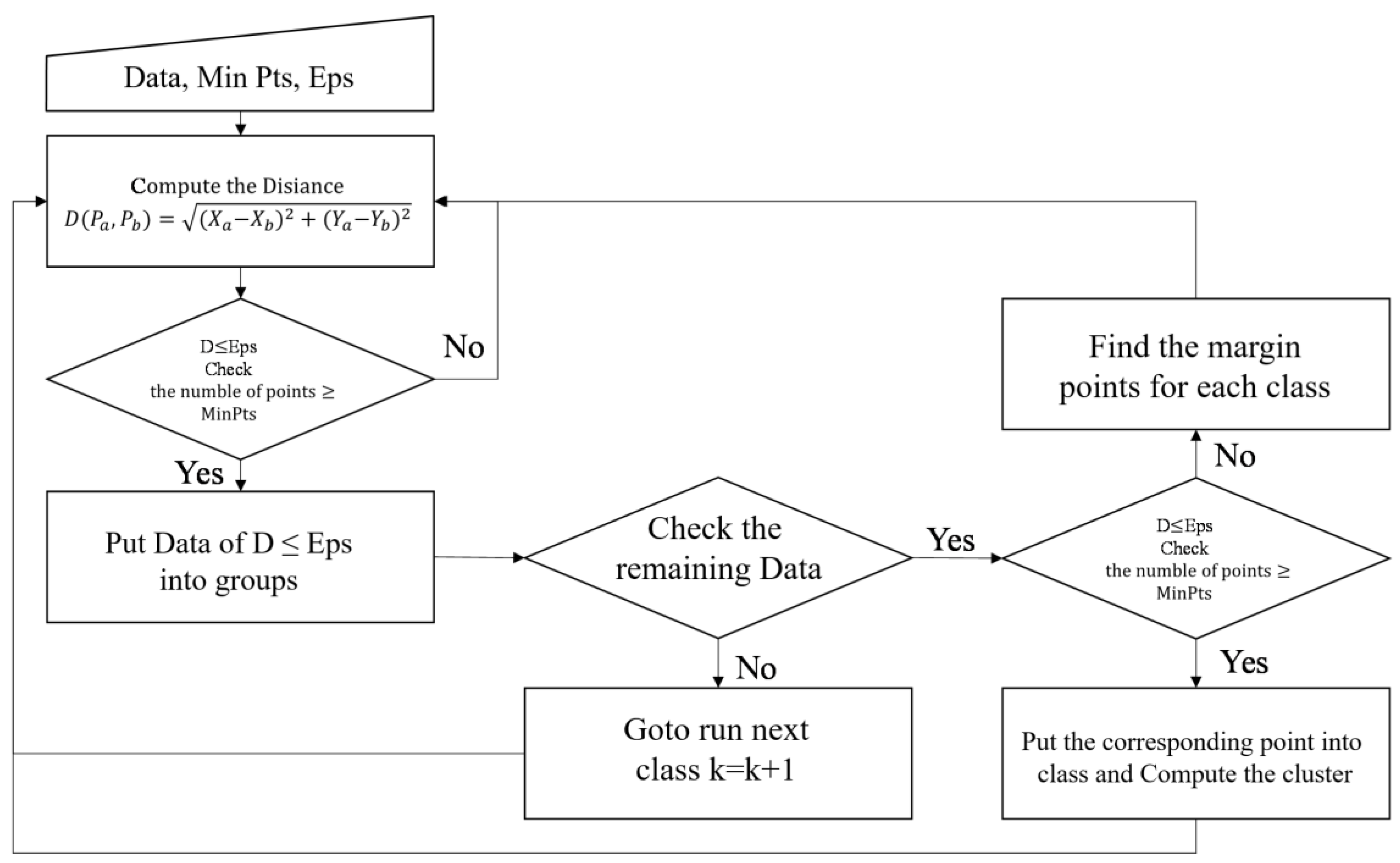
  • Outlier analysis of DBSCAN: as mentioned before, if a sample point does not fall in any of the ranges defined by the user, it is called an outlier or noise data. Since the DBSCAN algorithm can detect noise data, our developed program can be robust to outliers. In essence, the outlier analysis data in image classification are very important. Since the majority of the data could be observed by the main target category, a salt and pepper effect could also be significantly affected by the minor data. The DBSCAN can remove them to a list table. Figure 3 show steps for DBSCAN.

2.4.3. LDA

Linear discriminant analysis (LDA) is a classical statistical approach for classifying samples of unknown classes [11]. LDA is related to machine learning to find the linear combination of features which best separate two or more series of classes of objects. LDA can consider the measurements which are independent variables for various observations through continuous quantities. LDA is also to be viewed as an a priori process of data processing. Each case must have a score on one or more quantitative predictor measures and a score on a group measure. When dealing with categorical data, LDA is also different from factor analysis in that it is not an interdependent technique: a distinction between independent variables and dependent variables (also called criterion variables) must be made.

2.4.4. BPN

Neural networks are an information processing idea based on the way biological neural systems process data. Neural networks (NN) were first proposed in the early 1940s as a simulation of human brains’ cognitive learning processes [28]. They may be programmed so that the primary function is to develop various NN models of computer problems by trail and error or learning procedures. In the past twenty years, back propagation neural network were extensively applied in many fields. The relationship between massive data and a certain phenomenon is obtained through a learning system (instead of calculation), based on the neuron cell concept. Backpropagation is a widely used algorithm in training feedforward neural networks for supervised learning. Backpropagation computes the gradient of the loss function with corresponding weights of the network for a single input–output. This process makes it feasible to use gradient methods for training multilayer networks and updating weights to minimize loss is very popular. In the past, engineers and researchers experienced that the described variables for classifying remote sensing imagery are tough tasks. If a rice spatial image datum was well developed to describe the input variables and output categories rationally, it may be more suitable to apply a back propagation neural network as a learning machine.

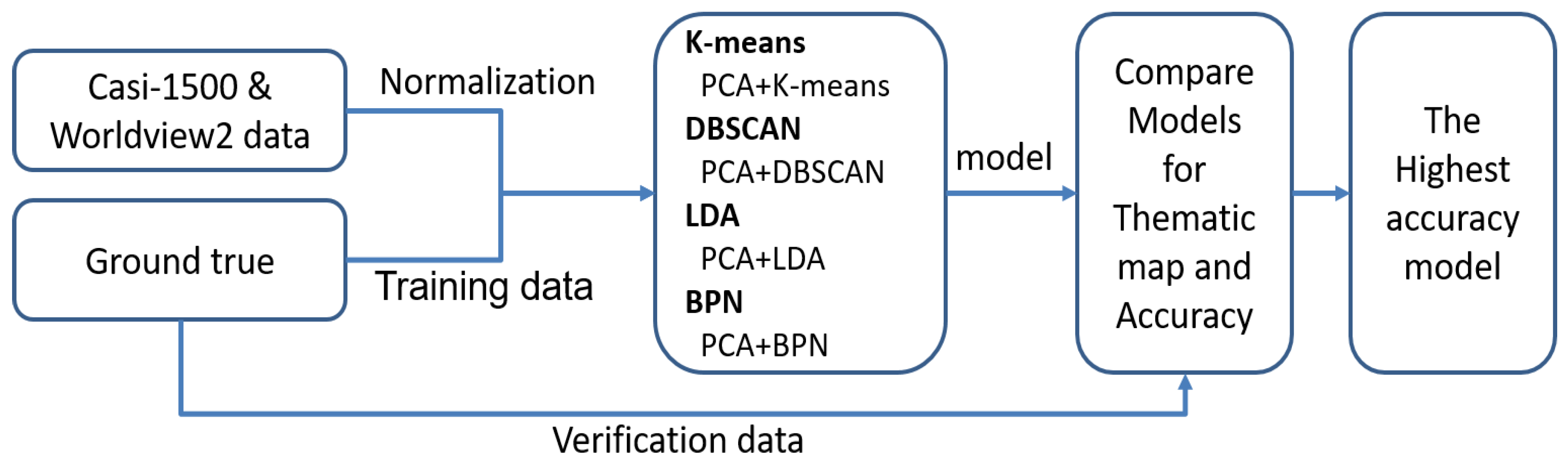
2.5. Data Pre-Processing with Evaluation Model

The model of our study contains DBSCAN, PCA, LDA and BPN four different approaches to understanding the different features between hyperspectral and multispectral data. LDA is a research method by attempting to use a single dependent variable as a linear combination to demonstrate features and measurements. We randomly and uniformly selected 500 training data items and 2000 testing data items for which a dataset was ready to verify the models. The research steps are shown in Figure 3. In Figure 3, the normalization process will arrange all the corresponding data to [−1, 1] by Equation (1):
X inew = 1   2 ( X i X m i n ) ( X m a x X m i n )
The research was designed to use PCA as a pre-processing tool to select the influenced attributes of the image spectral among 72 bands. While various attributes were selected, the classifier was adopted to present different classification outcomes. There are four classification methods for the test. The first classifier is the K-means as a tool to discern the paddy rice area. As part of this study, the DBSCAN was also applied as a classifier to approach the image classification on paddy rice. On the other hand, the LDA and BPN was used as a parallel study to compare the diversity outcomes from an image classifier. The data processing is shown in Figure 4, PCA has the function of attribute reduction, which can reduce the signal-to-noise ratio. Therefore, we also discuss PCA for LDA, DBSCAN and BPN groups, respectively, to check the difference in the data. The study will use κ and overall accuracy to calculate which classification method has better results.

3. Results and Discussion

This experiment was based on the farmland data that were investigated in the field. This experiment focused on the use of appropriate mathematical algorithms to improve the classification accuracy of classification among rice and other crop types. The above process will classify the sample: if it is similar to rice, it is classified into rice (replaced with rice); otherwise, the program will assign it in other types. In the supervised classification, 500 training samples and 2000 verification test samples are randomly selected to verify the model established by the training data. It is considered that some bands may not be suitable for parameter modeling. Therefore, the band is reduced in the PCA process and then classified. As mentioned above, 46 of the 72 bands that are factors are reduced to extract the performance of classification by the PCA approach. It is decided to set the 70% maximum eigenvalues of 72 bands (selected by PCA) to compare the research accuracy and it determines whether the classification effect will improve or not. The data handler must assign K (centroid number), Minpts, and Eps, which are three independent initial tracking values to achieve the best accuracy. The program has an iterative loop that does not stop until the best precision is reached.

3.1. Generation of Thematic Map

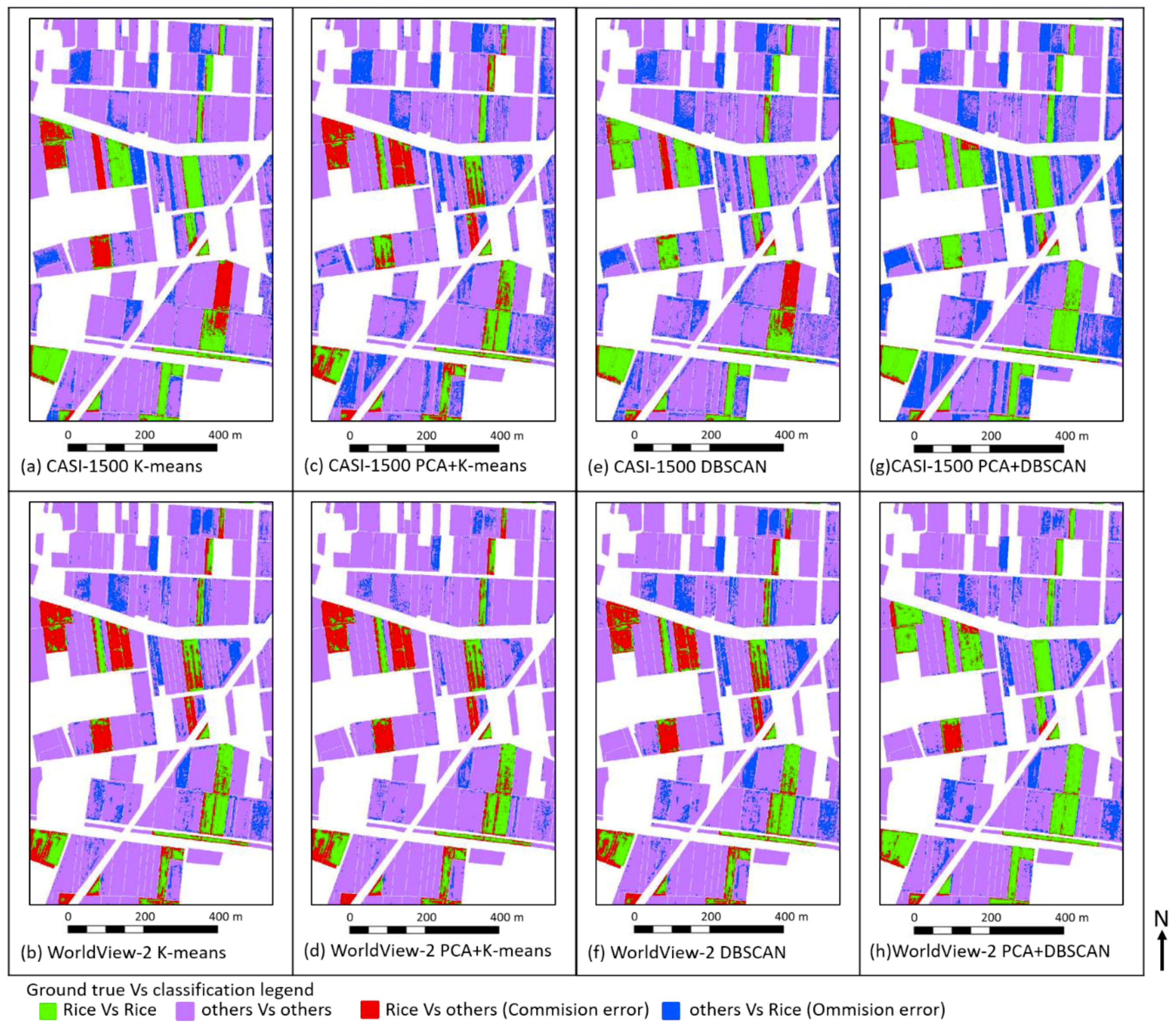
3.1.1. The Thematic Map Generated by K-Means

K-means and DBSCAN are both unsupervised learning approaches. Figure 5e–h present the thematic map of the full-size image classification of K-means on CASI-1500 and WorldView-2 with/without feature selection. For unsupervised learning, the label data were not requested for analysis which avoided a great amount of human in situ work for investigating. The thematic map is shown in Figure 5. In this figure, the thematic map is generated from the full-size image classification of K-means on CASI-1500 (hyperspectral) and WorldView-2 (multispectral) with/without feature selection. By using PCA for preprocessing, the hyperspectral data performed better than those of multispectral data. From the observations of the thematic map, most of the paddy rice area was integrity.

3.1.2. The Thematic Map Generated by DBSCAN

Figure 5e–h present the thematic map of the full-size image classification of DBSCAN on CASI-1500 and WorldView-2 with/without feature selection. The density-based clustering algorithm will adjust the factor of K (number of centroids) and Eps is used to obtain the highest accuracy classification result. The final parameter of inputs is selected by the combination of MinPts = 2, Eps = 0.05 as the best for the hyperspectral data. The combination of MinPts = 5, Eps = 0.35 was selected as the best for the hyperspectral data. This outcome was derived from the iteration search varying MinPts from 2 to 25 at 0.05 per iteration and Eps from 0.05 to 1.5 at 0.05 per iteration. The minimal error was attained step by step by following the previous ranges for MinPts and Eps. This figure is generated by following a similar process in Figure 5. Figure 5 is an unsupervised learning approach. The outcomes are clearly compared with two important conclusions: (a) hyperspectral image data interpret the classification outcomes much better than the multispectral image data; (b) DBSCAN provides better both in hyperspectral image data and multispectral image data by considering the results of solving the outlier data. The red parts (commission error) and blue parts (omission error) in Figure 5. This implies that the DBSCAN has better performance in classification than those of K-means. The feature selection method (PCA) does not display well for the K-means analysis. The outcome of DBSCAN is a little bit higher than that of K-means. The DBSCAN handles the outlier data much better than the K-means, especially when a proper EPS and radius are selected.

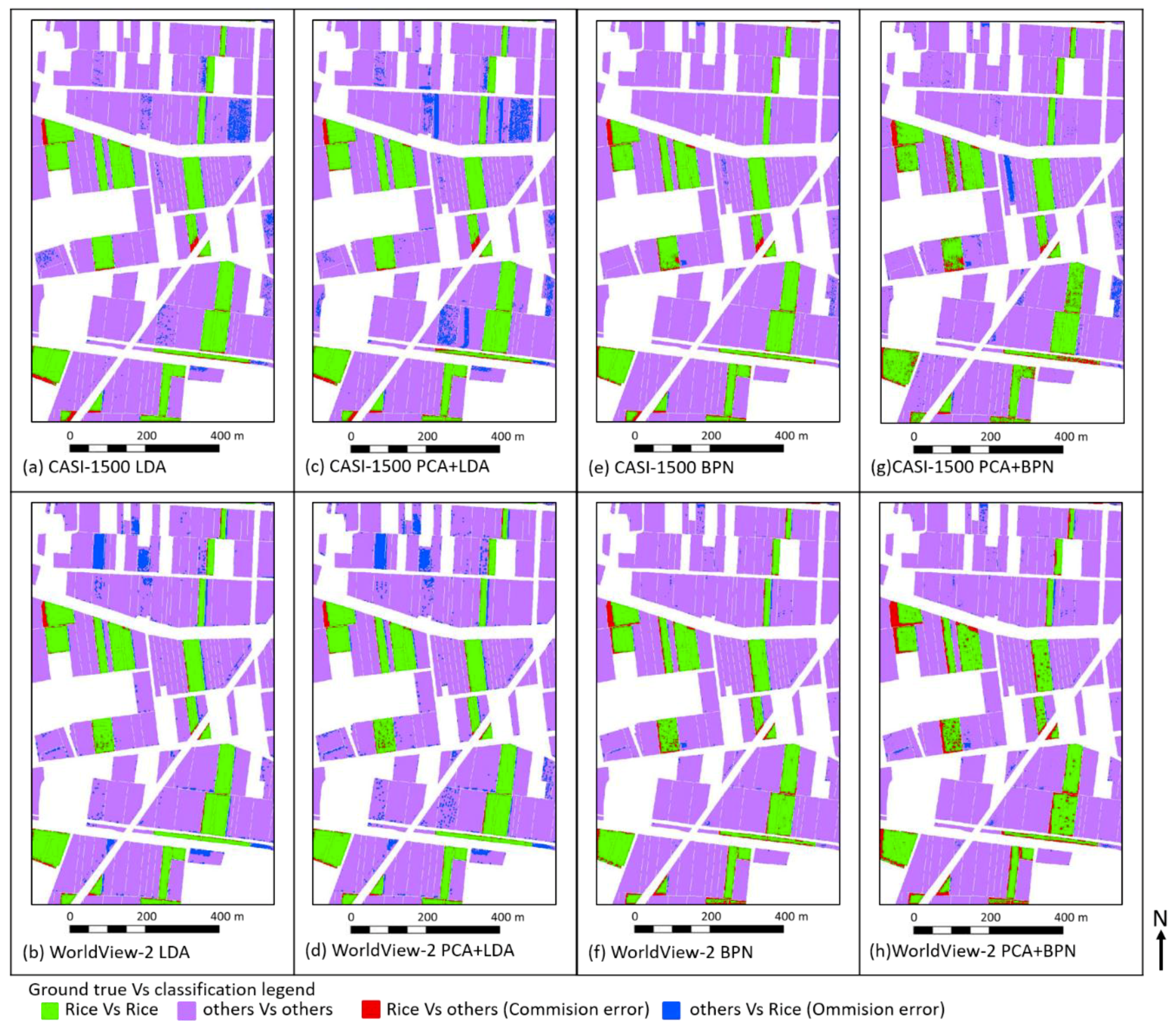
3.1.3. The Thematic Map Generated by LDA

This study used the Fisher’s linear discriminant, which is a statistics and machine learning approach to find a linear combination of features. Figure 6a–d present the thematic map of the full-size image classification of the LDA on CASI-1500 and WorldView-2 with/without feature selection. This clearly separates two or more classes of objects or events. PCA does not change much or improve the LDA approach of feature selection compared to Figure 5 and Figure 6. Figure 6 has very few red parts (commission error). The omission error displays many places on the thematic maps of considering/ignoring feature selection. Applying both hyperspectral and multispectral materials, it also displays an omission error much larger than the commission error. LDA clearly improves the accuracy rate of classification. However, the computational time of LDA is 6.5 times more than DBSCAN.

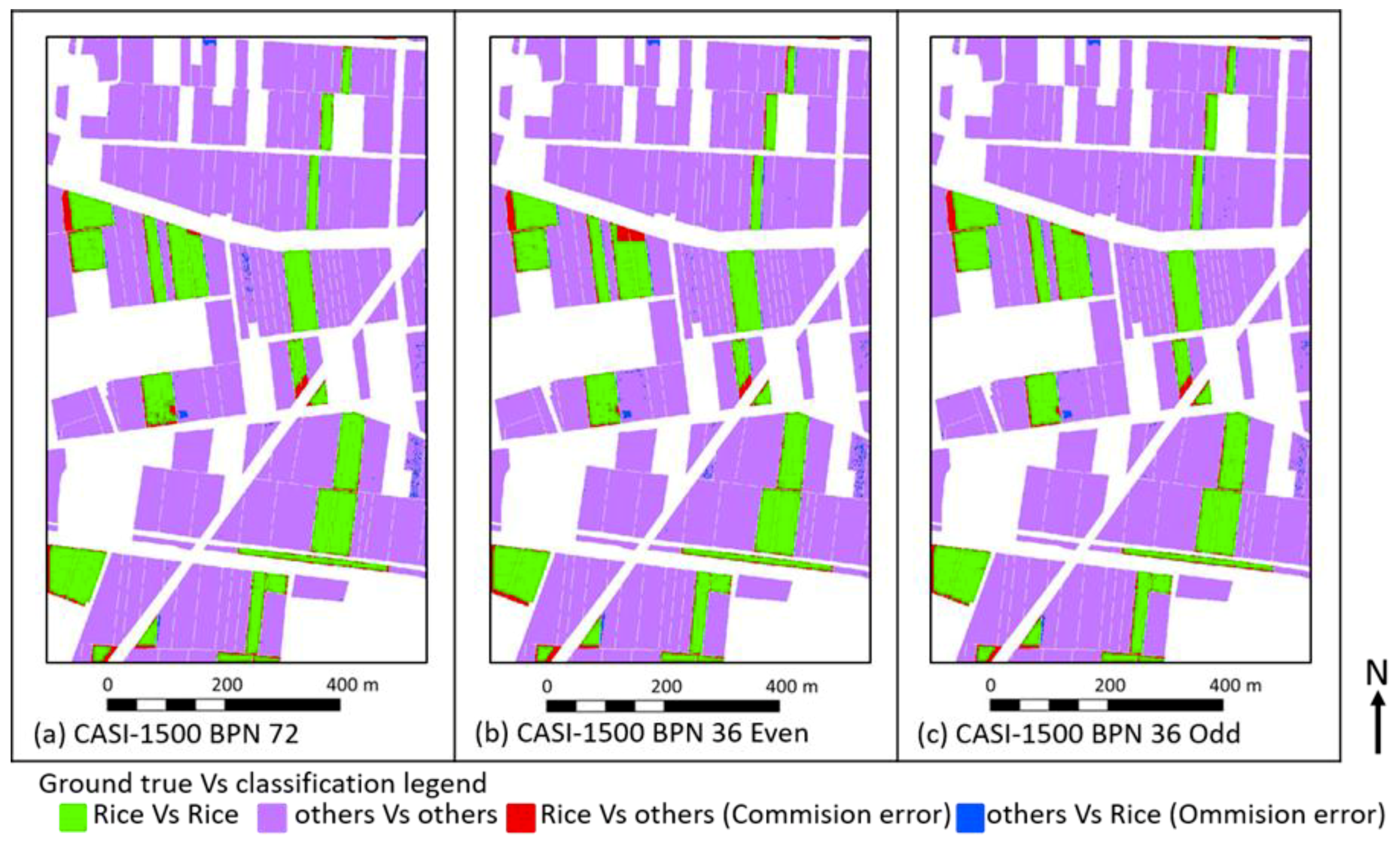
3.1.4. The Thematic Map Generated by BPN

Figure 6e–h present the thematic map of the full-size image classification of BPN on CASI-1500 and WorldView-2 with/without feature selection. In Figure 6e-g, it can be observed whether it has missed or misjudged the quite small proportion. Most of the errors come from the edge of the field area. As observed in Figure 6f,h, the process through PCA does not improve the classification accuracy. BPN obtains the best accuracy among the four classification methods. Neural networks have a calculation of iteration, so the classification result of the image will not be affected by the time difference between the image capture and field survey (Figure 1e).
This study wanted to explore if the original 72 bands are then divided into odd and even bands of 36 bands for the two different cases. Then, it was decided to compare the differences in data patterns to the classification results. The thematic map of the study is shown in Figure 7. Figure 7 shows that there are only small differences between the 72 bands, odd arrays, and even tissues, with no significant difference. Studies have shown that data analysis with BPN yields similar results.
From the experience of long-term field observation, we find that the edge area may be mainly affected by the following factors and shown in the Figure 8. There are some possible reasons for poor classification: (a) different planting directions; (b) paddy rice not full; (c) weed pixels interference, and different degrees of sunlight; (d) uneven fertilizer application, mainly the location of the outlet or inlet of the irrigation water which will affect the distribution of fertilizer in the field to varying degrees; (e) poor growth of machine channels, the tiller passes through the squeezing position repeatedly, and the soil becomes denser; or (f) the growth rate of the paddy rice is different. Therefore, the growth of the edge area is relatively inconsistent compared to the middle position. In addition, it is also possible that the information on the hill block of agricultural land utilization is summarized as paddy rice in the entire block, so even the surrounding area is indeed not paddy rice, and the classification result is also classified as non-paddy rice, but matching with the ground truth information will be classified as the omission error.

3.2. The Error Matrix for Accuracy

Table 2 shows the accuracy of 2000 verification samples of K-means, LDA, DBSCAN, and BPN (with/without PCA). It was found that BPN had the highest classification accuracy, the overall accuracy reaching 98%, followed by LDA, with an overall accuracy of 96%. Among the unsupervised classification methods, the PCA + DBSCAN had the higher overall accuracy (90%). Moreover, the DBSCAN could identify paddy rice areas without in situ investigation. It had been shown that the PCA plays an important role in DBSCAN in hyperspectral data than in multispectral data. It displays better agreements for accurate outcomes for hyperspectral data. This study summarizes the prominent function of PCA which is quite important for clustering analysis (DBSCAN), than the supervised classification analysis. Especially for a mass volume of data such as hyperspectral data. Since Worldview-2 or CASI-1500 images were taken during the reproductive period of rice, rice in different mounds has a non-synchronized growth state. For example, Park et al. [6] used time-series multispectral images for the field rice classification research. The research collected 11 multispectral images (Landsat) from before planting (March) to after the harvest (September) of rice. His study used support vector machines for supervised classification to analyze and compare the accuracy of rice classification in each period. Their results show that the classification accuracy of different growth stages will be different. For example, the classification accuracy of just the planting stage is 72~81%, the classification accuracy of the growth stage is 90~97%, and the harvest stage is 78~88%. The images used in this study are close to the upcoming harvest. Unsupervised classification does not have the characteristics of training samples like supervised classification. Therefore, the classification performance is slightly lower, which is accepted.
Table 2 also shows the results of the verification accuracy of four actual true evidences, and Figure 5, Figure 6 and Figure 7 show a graphical representation of the accuracy of full-frame image verification. Comparing the difference between the two different verification areas (2000 random sampling data and 323,600-pixel data in the whole area) in Table 2, the results show that the overall average accuracy of Table 2 is quite similar, it decreased the mean from 0.4 to 2.8%. In this area, it was decided to consider the four different models mentioned previously. Similar to the previous calculation, the K-means with/without feature selection of PCA attain about 82~84% accuracy vs. 80~81%, respectively. The DBSCAN is also an unsupervised approach which presents about 4.9~6.0% accuracy compared to the K-means. The LDA and BPN are a supervised approach which requests a series of label data of previous preparing works. These preparing works of in situ investigation are very time-consuming for large training datasets. In addition, the computational time of the huge training data is many times larger than DBSCAN.

4. Conclusions

Paddy rice is an important crop that plays a crucial role in agriculture in Taiwan. Different image data with a suitable image classification model is very helpful to determine the area and location of paddy rice. On the other hand, different classification models may result in various classification outcomes with different image material which draw great attention from scientists and scholars. Therefore, this study analyzes multispectral (WorldView-2) and hyperspectral images (CASI-1500) of a typical agricultural land in Yunlin County, Taiwan. The study uses unsupervised classification algorithms of K-means and PCA and supervised classification algorithms of LDA and DBSCAN for rice image classification. The image data and ground truth data of our study area are well recorded and verified.
The advantage of using DBSCAN is that it does not need to pre-request given categories. That is, it greatly reduces a huge amount of in situ works. In addition, it renders better K-means classification. The DBSCAN approach performs about 5.4% better classification outcomes than those of K-means. It also saves a great amount of the computational time to only 15% (such as comparing to LDA). The DBSCAN with considering the feature selection (PCA) can attain an about accuracy of 90% and also save 95.1% of the computational time which compares to BPN. Although, the flaw of this method is that the accuracy cannot be compared to a supervised learning model, such as BPN. To sum up, DBSCAN can widely be applied to the geosciences of remote sensing without a large number of preprocessing calculations and parameter screening is a good model to save labor time and cost, as well as for fast classification.
Among all the approaches, the results show that the BPN, which is a supervised approach, has the highest accuracy for rice classification in hyperspectral and multispectral. With a κ of 0.90 and an overall classification accuracy of 97%, hyperspectral is better than those of the multispectral. The accuracy of other classifications is significantly lower. For LDA, even if the status of CASI-1500 and WorldView-2 have a different record on the field investigations, but the classification outcomes are still well modeled by BPN.
Comparing the image data of the supervised and unsupervised classification, the hyperspectral classification accuracy is better than that of multispectral image classification since the hyperspectral has more information to interpret the in situ investigation. Different approaches are presented and hyperspectral and multispectral images are both employed to show their differences in error matrix and thematic maps. In this study, one can observe the classification and track the distribution status of the error information. PCA for feature selection will slightly reduce the accuracy but greatly improve the computation efficiency. BPN is the best classifier in the supervised approach.

Author Contributions

S.W. was responsible for the concept, design and most of the writing and review of the manuscript, and participated in the linear discriminant analysis, density-based clustering algorithms, and the back propagation and data analysis. Y.-P.W. mainly processed and analyzed the multispectral and hyperspectral images, organized graphics, statistical and verification forms, and participated in writing and editing the manuscripts. All authors have read and agreed to the published version of the manuscript.

Funding

This research was funded by [Ministry of Science and Technology, Taiwan] grant number [106-2119-M-275-002] and [106-2313-B-005-013].

Conflicts of Interest

The authors declare no conflict of interest.

References

  1. Wang, Y.P.; Chang, K.-W.; Chen, R.-K.; Lo, J.-C.; Shen, Y. Large-area rice yield forecasting using satellite imageries. Int. J. Appl. Earth Obs. Geoinf. 2010, 12, 27–35. [Google Scholar] [CrossRef]
  2. Wang, Y.P.; Shen, Y. Identifying and characterizing yield limiting soil factors with the aid of remote sensing and data mining techniques. Precis. Agric. 2015, 16, 99–118. [Google Scholar] [CrossRef]
  3. Wan, S. A spatial decision support system for extracting the core factors and thresholds for landslide susceptibility map. Eng. Geol. 2009, 108, 237–251. [Google Scholar] [CrossRef]
  4. Coca, F.C.-D.; García-Haro, F.J.; Gilabert, M.A.; Melia, J. Vegetation cover seasonal changes assessment from TM imagery in a semi-arid landscape. Int. J. Remote Sens. 2004, 25, 3451–3476. [Google Scholar] [CrossRef]
  5. Steele, B. Combining Multiple Classifiers: An Application Using Spatial and Remotely Sensed Information for Land Cover Type Mapping. Remote Sens. Environ. 2000, 74, 545–556. [Google Scholar] [CrossRef]
  6. Park, S.; Im, J.; Park, S.; Yoo, C.; Han, H.; Rhee, J. Classification and Mapping of Paddy Rice by Combining Landsat and SAR Time Series Data. Remote Sens. 2018, 10, 447. [Google Scholar] [CrossRef] [Green Version]
  7. Anys, H.; He, D.-C. Evaluation of textural and multipolarization radar features for crop classification. IEEE Trans. Geosci. Remote Sens. 1995, 33, 1170–1181. [Google Scholar] [CrossRef]
  8. Pradhan, B. A comparative study on the predictive ability of the decision tree, support vector machine and neuro-fuzzy models in landslide susceptibility mapping using GIS. Comput. Geosci. 2013, 51, 350–365. [Google Scholar] [CrossRef]
  9. Breim, G.J.; Benediktsson, J.A.; Sveinsson, J.R. Multiple classifiers applied to multisource remote sensing data. IEEE Trans. Geosci. Remote Sens. 2002, 40, 2291–2299. [Google Scholar] [CrossRef] [Green Version]
  10. Xu, M.; Watanachaturaporn, P.; Varshney, P.K.; Arora, M.K. Decision tree regression for soft classification of remote sensing data. Remote Sens. Environ. 2005, 97, 322–336. [Google Scholar] [CrossRef]
  11. Wan, S.; Chang, S.-H. Combined particle swarm optimization and linear discriminant analysis for landslide image classification: Application to a case study in Taiwan. Environ. Earth Sci. 2014, 72, 1453–1464. [Google Scholar] [CrossRef]
  12. Carr, J.R. Spectral and textural classification of single and multiple band digital images. Comput. Geosci. 1996, 22, 849–865. [Google Scholar] [CrossRef]
  13. Carpenter, G.; Gjaja, M.; Gopal, S.; Woodcock, C. ART neural networks for remote sensing: Vegetation classification from Landsat TM and terrain data. IEEE Trans. Geosci. Remote Sens. 1997, 35, 308–325. [Google Scholar] [CrossRef] [Green Version]
  14. Benediktsson, J.A.; Swain, P.H.; Esroy, O.K. Neural network approaches versus statistical methods in classification of multisource remote sensing data. IEEE Trans. Geosci. Remote Sens. 1990, 28, 540–552. [Google Scholar] [CrossRef]
  15. Vinodhini, G.; Chandrasekaran, R.M. A comparative performance evaluation of neural network based approach for sentiment classification of online reviews. J. King Saud Univ. Comput. Inf. Sci. 2016, 28, 2–12. [Google Scholar] [CrossRef] [Green Version]
  16. Yu, S.; Backer, S.D.; Scheunders, P. Genetic feature selection combined with composite fuzzy nearest neighbor classifiers for high-dimensional remote sensing data. In Proceedings of the IEEE International Conference on Systems, Man & Cybernetics, Nashville, TN, USA, 8–11 October 2000; pp. 1912–1916. [Google Scholar]
  17. Cheriyadat, A.; Bruce, L.M. Why principal component analysis is not an appropriate feature extraction method for hyperspectral data. In Proceedings of the IEEE International Geoscience and Remote Sensing Symposium, Toulouse, France, 21–25 July 2003; pp. 3420–3422. [Google Scholar]
  18. Bárdossy, A.; Samaniego, L. Fuzzy rule-based classification of remotely sensed imagery. IEEE Trans. Geosci. Remote Sens. 2002, 40, 362–374. [Google Scholar] [CrossRef]
  19. Lu, D.; Mausel, P.; Batistella, M.; Morán, E. Land-cover binary change detection methods for use in the moist tropical region of the Amazon: A comparative study. Int. J. Remote Sens. 2005, 26, 101–114. [Google Scholar] [CrossRef]
  20. Collin, A.; Lambert, N.; Etienne, S. Satellite-based salt marsh elevation, vegetation height, and species composition mapping using the superspectral WorldView-3 imagery. Int. J. Remote Sens. 2018, 39, 5619–5637. [Google Scholar] [CrossRef]
  21. Hartling, S.; Sagan, V.; Sagan, V.; Maimaitijiang, M.; Carron, J. Urban Tree Species Classification Using a WorldView-2/3 and LiDAR Data Fusion Approach and Deep Learning. Sensors 2019, 19, 1284. [Google Scholar] [CrossRef] [Green Version]
  22. Wan, S.; Lei, T.; Huang, P.; Chou, T. The knowledge rules of debris flow event: A case study for investigation Chen Yu Lan River, Taiwan. Eng. Geol. 2008, 98, 102–114. [Google Scholar] [CrossRef]
  23. Senthilnath, J.; Omkar, S.N.; Mani, V.; Karnwal, N.; Shreyas, P.B. Crop Stage Classification of Hyperspectral Data Using Unsupervised Techniques. IEEE J. Sel. Top. Appl. Earth Obs. Remote Sens. 2012, 6, 861–866. [Google Scholar] [CrossRef]
  24. Massarelli, C.; Matarrese, R.; Uricchio, V.F.; Muolo, M.R.; Laterza, M.; Ernesto, L. Detection of asbestos-containing materials in agro-ecosystem by the use of airborne hyperspectral CASI-1500 sensor including the limited use of two UAVs equipped with RGB cameras. Int. J. Remote Sens. 2017, 38, 2135–2149. [Google Scholar] [CrossRef]
  25. Bertels, L.; Vanderstraete, T.; Van Coillie, S.; Knaeps, E.; Sterckx, S.; Goossens, R.; Deronde, B. Mapping of coral reefs using hyperspectral CASI data; a case study: Fordata, Tanimbar, Indonesia. Int. J. Remote Sens. 2008, 29, 2359–2391. [Google Scholar] [CrossRef]
  26. Blei, D.M.; Ng, A.Y.; Jordan, M.I. Latent Dirichlet Allocation. J. Mach. Learn. Res. 2003, 3, 993–1022. [Google Scholar]
  27. Vellido, A.; Lisboa, P.J.G.; Vaughan, J. Neural Networks in Business: A Survey of Applications (1992–1998). Expert Syst. Appl. 1999, 17, 51–70. [Google Scholar] [CrossRef]
  28. Gupta, J.N.; Stafford, E.F. Flowshop scheduling research after five decades. Eur. J. Oper. Res. 2006, 169, 699–711. [Google Scholar] [CrossRef]
  29. Peres-Neto, P.R.; Jackson, D.A.; Somers, K.M. How many principal components? Stopping rules for determining the number of non-trivial axes revisited. Comput. Stat. Data Anal. 2005, 49, 974–997. [Google Scholar] [CrossRef]
  30. Sander, J.; Ester, M.; Kriegel, H.-P.; Xu, X. Density-Based Clustering in Spatial Databases: The Algorithm GDBSCAN and Its Applications. Data Min. Knowl. Discov. 1998, 2, 169–194. [Google Scholar] [CrossRef]
  31. MacQueen, J.B. Some Methods for classification and Analysis of Multivariate Observations. In Proceedings of the 5th Berkeley Symposium on Mathematical Statistics and Probability; University of California Press: Berkeley, CA, USA, 1967; pp. 281–297. [Google Scholar]
  32. Birant, D.; Kut, A. ST-DBSCAN: An algorithm for clustering spatial–temporal data. Data Knowl. Eng. 2007, 60, 208–221. [Google Scholar] [CrossRef]
  33. Kriegel, H.; Kröger, P.; Sander, J.; Zimek, A. Density-based clustering. Wiley Interdiscip. Rev. Data Min. Knowl. Discov. 2011, 1, 231–240. [Google Scholar] [CrossRef]
  34. Tran, T.N.; Drab, K.; Daszykowski, M. Revised DBSCAN algorithm to cluster data with dense adjacent clusters. Chemom. Intell. Lab. Syst. 2013, 120, 92–96. [Google Scholar] [CrossRef]
  35. Schubert, E.; Sander, J.; Ester, M.; Kriegel, H.P.; Xu, X. DBSCAN Revisited, Revisited. ACM Trans. Database Syst. 2017, 42, 1–21. [Google Scholar] [CrossRef]
  36. Tian, Y.; Ye, B.; Wan, L.; Yang, M.; Xing, D. Restricted Airspace Unit Identification Using Density-Based Spatial Clustering of Applications with Noise. Sustainability 2019, 11, 5962. [Google Scholar] [CrossRef] [Green Version]
Figure 1. The study area images and ground truth. (a) WorldView-2; (b) CASI1500; (c) Ground True; (d) Sample Site; and (e) Data times and rice growth status.
Agriculture 10 00465 g001
Figure 2. Visualize the steps for density-based spatial clustering of applications with noise (DBSCAN). (a) Parameter illustration; (b) Direct density can approach; (c) Indirect linkage by density; and (d) The linkage by density.
Agriculture 10 00465 g002
Figure 3. Steps for DBSCAN.
Agriculture 10 00465 g003
Figure 4. Research Steps. This study used multispectral images (WorldView-2) and hyperspectral images (CASI-1500) and focused on the classifiers K-means, density-based spatial clustering of applications with noise (DBSCAN), linear discriminant analysis (LDA), and back-propagation neural network (BPN). Then the feature selection (principle component analysis, PCA) on four classifiers is studied.
Agriculture 10 00465 g004
Figure 5. Thematic map of the full-size image unsupervised classification of the K-means and DBSCAN on CASI-1500 (hyperspectral) and WorldView-2 (multispectral) with/without feature selection. (a) CASI-1500 K-means; (b) WorldView-2 K-means; (c) CASI-1500 PCA+K-means; (d) WorldView-2 PCA+K-means; (e) CASI-1500 DBSCAN; (f) WorldView-2 DBSCAN; (g) CASI-1500 PCA+DBSCAN; and (h) WorldView-2 PCA+DBSCAN.
Agriculture 10 00465 g005
Figure 6. Thematic map of the full-size image supervised classification of LDA and BPN on CASI-1500 (hyperspectral) and WorldView-2 (multispectral) with/without feature selection. Note: the red parts are rice, classified as other categories (commission error). The blue parts are others, classified as rice (omission error). (a) CASI-1500 LDA; (b) WorldView-2 LDA; (c) CASI-1500 PCA+LDA; (d) WorldView-2 PCA+LDA; (e) CASI-1500 BPN; (f) WorldView-2 BPN; (g) CASI-1500 PCA+BPN; and (h) WorldView-2 PCA+BPN.
Agriculture 10 00465 g006
Figure 7. Thematic map of the full-size image classification of BPN on CASI-1500 (hyperspectral) with the different bands. Note: the red parts are rice, classified as other categories (commision error). The blue parts are others, classified as rice (ommision error). (a) CASI-1500 BPN 72; (b) BPN 36 Even; and (c) BPN 36 Odd.
Agriculture 10 00465 g007
Figure 8. Possible reasons for poor classification: (a) different planting directions; (b) paddy rice not full; (c) weed pixels interference; (d) uneven fertilizer application; (e) poor growth of machine channels; and (f) the growth rate of paddy rice is different.
Agriculture 10 00465 g008
Table 1. The full width at half maximum (FWHM) of each band and the best accuracy of the clustering center of multispectral (8 bands) and the hyperspectral data.
Multispectral (WorldView-2)Hyperspectral (CASI-1500)
BandsCentre (nm)FWHM (nm)Paddy Rice Cluster CenterBandCentre (nm)FWHM (nm)Paddy Rice Cluster Center
Coastal42525−0.76681370.74.8−0.2697
Blue48030−0.77292380.24.8−0.4077
Green54535−0.49593389.84.8−0.4064
Yellow60520−0.65574399.34.8−0.5165
Red66030−0.80555408.94.8−0.6197
Red Edge725200.3295
NIR1832.562.50.4875681008.34.80.3325
NIR2950900.4907691017.84.80.3204
701027.34.80.3045
711036.84.80.3730
721046.34.80.3423
Table 2. Accuracy of 2000 verification samples. Statistical results of full-frame image verification accuracy (total 323,600 pixels).
2000 Samples Verification AccuracyFull-Frame Image Verification Accuracy
Image TypeStudy WayKappaMeanOA * (%)MeanKappaMeanOA (%)Mean
Casi-1500K-means0.640.5086.7080.380.470.4184.2683.21
WorldView2K-means0.3574.050.3582.16
Casi-1500PCA + K-means0.450.4678.5579.680.440.3980.7980.95
WorldView2PCA + K-means0.4780.800.3481.11
Casi-1500DBSCAN0.740.6489.3086.380.600.6386.4888.09
WorldView2DBSCAN0.5583.450.6589.70
Casi-1500PCA + DBSCAN0.830.7792.7090.150.570.5685.0486.97
WorldView2PCA + DBSCAN0.7187.600.5688.91
Casi-1500LDA0.930.9397.1096.900.850.8495.7295.34
WorldView2LDA0.9296.700.8394.96
Casi-1500PCA + LDA0.930.9297.1096.630.790.8093.5993.81
WorldView2PCA + LDA0.9196.150.8094.03
Casi-1500BPN0.980.9799.3598.630.900.8997.2896.96
WorldView2BPN0.9597.900.8896.64
Casi-1500PCA + BPN0.910.8996.1595.530.820.8295.2195.11
WorldView2PCA + BPN0.8794.900.8195.02
Casi-1500BPN720.980.9899.3599.30.900.9097.2897.25
Casi-1500BPN 36 odd0.9999.550.9097.37
Casi-1500BPN 36 even0.9899.000.8997.11
* OA: Overall accuracy.

