On the Way to Sustainable Agriculture—Eco-Efficiency of Polish Commercial Farms

Abstract

The negative impact of agriculture on the natural environment is not a new issue. One of the ideas to overcome this problem is the eco-efficiency concept, analyzing the agricultural output in relation, not only to traditional inputs, but to the environmental impact, as well. This paper aims at calculating the eco-efficiency of Polish commercial farms, based on a representative sample of 601 farms participating in the Polish Farm Accountancy Data Network (FADN). To assess the eco-efficiency of the farms, variables illustrating traditional inputs (land, labor, capital), as well as variables reflecting the environmental pressure of the surveyed farms (greenhouse gas (GHG) emissions, and nitrogen and phosphorus surpluses) were used. Data envelopment analysis (DEA) revealed that, on average, farms could reduce their inputs by almost a quarter without reducing their outputs. Additionally, it was revealed that incorporating externalities of agricultural production into analyses decreases the diversity of the farm population in terms of efficiency measures. According to the analyses, more eco-efficient farms are characterized by larger utilized agricultural area (UAA), higher production value, and higher intensity of chemical inputs per 1 ha, but at the same time by lower amounts of inputs used per production unit. Moreover, more eco-efficient farms achieved higher farm incomes in many terms: total, per 1 ha of UAA, and per 1 EUR of production value.

1. Introduction

For most of humankind’s history, due to the small number of people inhabiting the Earth, our environmental impact was usually local, but the fast growth of the human population observed in the 20th century changed the situation [1]. Growing demand for food, which has been satisfied thanks to the “green revolution”, increased the pressure of agriculture on the natural environment [2,3,4,5,6]. However, taking into account the constant growth of the human population [7], it is not possible to reduce the negative environmental impact of agriculture through the reduction of food production. Thus, the only possible solution is to reduce the negative consequences of agricultural production through implementing more environmentally friendly production techniques, as is postulated by the promoters of sustainable agriculture [8,9,10].

One of the ways to operationalize sustainability assumptions is eco-efficiency [11,12]. This concept searches for production solutions that will cause the highest possible reduction in use of natural resources, while maintaining or even increasing the production level. As an idea, it reflects the willingness to do “more with less: delivering more value while using fewer resources” [13] (p. 4); on the analytical level it means using such methods of assessing the efficiency of economic processes that will also include their environmental impact. Since the 1990s the eco-efficiency concept has been used by industrial enterprises to assess the environmental impact of various economic actions and decisions [11]. With time, the original approach has been extended to non-industrial sectors and beyond single-company scales [14,15,16,17,18], and the concept became one of the methods used to operationalize the sustainability concept.

Taking into consideration challenges faced currently by agriculture, the necessity to reduce environmental impact on one hand [19,20,21,22], and growing world demand for food on the other [7], we can say that the eco-efficiency concept seems very promising. Thus, the main aim of this paper was the assessment of the eco-efficiency of Polish commercial farms, considering both types of farming outcomes: positive ones (agricultural production) and negative ones (environmental impact). The analyses are based on data envelopment analysis (DEA), where the traditional set of variables (agricultural land, labor, and capital as means of production) were supplemented by variables representing the environmental pressure (nitrogen and phosphorus surplus, as well as greenhouse gas (GHG) emissions). The eco-efficiency scores were further compared with a set of farm characteristics and their sustainability assessment (in environmental, economic, and social dimensions). The novelty of the paper is the comparison of overall farm eco-efficiency (including all inputs, conventional and environmental impact) with farm sustainability level. The assessment was carried out at the farm level to show that basic farm characteristics might be used to evaluate farm eco-efficiency in a simple and robust manner. Additionally, the potential of improving efficiency in different farms was assessed and compared to reveal farm diversity regarding the use of conventional input use, and also environmental impact.

1.1. The Environmental Impact of Agriculture

Technological progress observed in agriculture in the last few decades allows the satisfaction of constantly rising demand for food, but at the same time, it increases negative impact on the natural environment [6,23]. Farming participates in such negative phenomenon as disturbances in the natural circulation of nutrients (nitrogen and phosphorus), soil erosion, greenhouse gasses emissions, pollution of surface and ground waters, as well as the decline in biodiversity of ecosystems [24,25,26]. Liu et al. [27] (p. 2) stressed that “reducing nutrient pollution from agriculture remains challenging due to a large number of producers and the spatially variable and temporally dynamic nature of the nutrient loading process”. Of course, these negative processes are not exclusively caused by agriculture, but surely it has a significant impact on crossing some of the nine planetary boundaries [28,29]. The planetary boundary concept is aimed at defining the environmental limits within which humanity can safely operate [29]. Exceeding a certain level of impact includes, for example, pollution causing irreversible changes in the Earth ecosystems that will endanger the existence of all its inhabitants, including humankind. Steffen et al. [29] identified “biochemical flows” (phosphorus and nitrogen) and “genetic diversity” as elements beyond the zone of uncertainty, which put a high risk of pushing the Earth system into a new state. Additionally, the risk of climate change caused by GHG emissions remains essentially important in this context. Agriculture plays a very important role in all of these processes.

The disturbance of the circulation of nitrogen in the environment occurs when large quantities of reactive nitrogen, mainly from fertilization, leak into the soils and water [30,31,32,33]. Since 1961 the global use of nitrogen fertilizers has risen from about 11 million t to over 100 million t at the beginning of the 21st century [34]. Simultaneously, the efficiency of their use deteriorated significantly, as fertilizer consumption rises faster than the plant yields [34,35]. According to various sources, as much as 50–75% of nitrogen introduced into the soils by farmers can be lost to the environment [30,36,37]. The main results of this process are groundwater pollution and eutrophication of water reservoirs, leading to damage both to the natural environment and human health [38,39,40,41,42].

The second very negative impact of agriculture on the natural environment are disturbances in phosphorus circulation, resulting from its discharge into water reservoirs, due to agricultural soil erosion. According to the European Environment Agency—EEA [43], phosphorus leaching to freshwater due to agriculture activities in most of the European territory exceeds on average 0.1 kg/ha per year; reaching, in the most vulnerable places, even 1 kg/ha per year, also polluting the sea, especially coastal, waters. The high amount of this nutrient in water causes plankton blooms that might cause the death of fish and other water animals, further causing the health problems of death of fish and other water animals [44].

The third place in the adverse effects of agriculture on the natural environment is taken by GHG emissions. Globally, agriculture is responsible for about 11.2% of GHG emissions [45], not only carbon dioxide but methane (with greenhouse potential 21 times higher than the one represented by CO₂) and nitrous oxide (with greenhouse potential 310 times higher than the one represented by CO₂) [46]. According to The Food and Agriculture Organization—FAO [47], in 2012 global GHG emissions caused by agriculture (plant cultivation and animal breeding) reached 5.4 billion t of CO₂ equivalent; which was twice as much as in 1961. Globally, the highest GHG emissions in agriculture are as a result of enteric fermentation (40%), manure left on pasture (16%), synthetic fertilizers (13%), paddy rise (7%), and burning biomass on savannahs (5%) [47].

Agriculture is also the most important consumer of global freshwater resources, responsible for 70% of global freshwater withdrawals and more than 90% of its consumptive use [48]. Most of the water used in agriculture comes from precipitation, however, about 15% comes from irrigation. During the last 50 years the land irrigated has doubled, and currently, about 24% of the utilized agricultural area is irrigated [49]. Global water withdrawal for agricultural purposes is estimated at about 2469 km³ (including 1257 km³ used for production, of which only about 50% is used effectively) [50]. Land irrigation might result in soil salinity. It is estimated that between 20% and 50% of irrigated land is affected by salinity [51]. This might be a consequence of physiological drought, which means the inability to uptake the minerals from the soil by plants.

In many parts of the world, agriculture is responsible for deforestation aiming at obtaining new agricultural land. According to data gathered within the Global Carbon Project [52], deforestation results in 10% of global GHG emissions and a cumulative 3% of GHG emissions observed in the second half of the 20th century. Cutting down forests reduces the emission of volatile organic compounds that can cool the climate by dispersing solar radiation [53]. Moreover, according to the newest research, forests most probably play a fundamental role in water circulation, creating so-called “rivers in the sky” that transport water for long distances [54]. Ellison [55], as well as Wolosin and Hariss [56], suggested that deforestation brings more serious consequences to water circulation than to GHG emission.

Agriculture is also said to be the main cause of the loss of biodiversity [57,58]. According to the International Union for Conservation of Nature [59], agricultural production endangers the existence of 5407 out of 8688 species included on the “extinction red list”, including pollinators that are necessary for plant production.

This overview proves that the problem of agricultural impact on the natural environment lies not only in using natural resources, but mainly in its low efficiency: more efficient use of fertilizers could significantly reduce the scale of nitrogen and phosphorus surplus delivered to the environment; rational use of plant protection products could reduce biodiversity loss; better management of water resources and smarter crop planning could help to reduce water use by agriculture, and finally, increasing crop yields could reduce the pressure on cutting down forests to increase the agricultural area. Thus, it is necessary to look for methods to improve the efficiency of natural resource use in agriculture.

From the point of view of economics, the negative impact of agriculture on the natural environment results in negative externalities, which are a production cost paid not by the producer but by the rest of the society [60]. The term “externalities” was used as early as in the works of Marshall (1842–1924), but his idea was significantly developed by Pigou (1877–1959); referring to the welfare theory he claimed, that the existence of externalities results from a disparity between private and public benefits on the one hand, and private and public costs on the other [61].

The concept of externalities is most often used referring to external costs, but there are also external benefits possible [62]. Both positive and negative externalities are a result of market failure, resulting in inefficient (in a Pareto sense) allocation of resources, which in consequence leads to a disparity between the economic and social optimum [63]. The existence of externalities leads to the lack of equilibrium and inability to reach the Pareto optimum, and in consequence to ineffective resource allocation (too large or too small amounts of resources are assigned to particular types of activities because market signals are in such a situation imperfect) [64].

In this context, it is worth emphasizing that the endeavor to achieve Pareto effectiveness (through eliminating market failures, seen as externalities) in the economy as a whole might simultaneously cause inefficiency on the level of a company (or a farm). For a single unit, the ability of externalization of externalities might result in a competitive advantage in comparison with other units, that do not externalize their side effects. Thus, it is important to assess the efficiency of units using not only traditional production factors but the “use of natural resources” (in the form of negative externalities) as well.

1.2. The Eco-Efficiency Concept as a Tool to Realize Sustainable Development

Scholars and policy-makers for a long time were concerned with the problems of the natural environment and quality of life, in connection with technical development and civilizational progress. Among other possible solutions, the concept of sustainable development was created. Modern discussion on this concept emerged after 1987 when the World Commission on Environment and Development (also called the “Brundtland Commission”) published its report. It contained the most often cited definition of sustainable development, according to which the main goal of sustainability is “to ensure that it meets the needs of the present without compromising the ability of future generations to meet their own needs” [65] (p. 54).

However, the resources that should be available should not be treated in the narrow sense as raw material, but also regarding their contribution to the quality of the surrounding environment (air quality, biodiversity, etc.). The key issue is to simultaneously consider three sustainability dimensions, that is economic, environmental, and social issues; which means that all actions should be environmentally rational, economically sound, and socially acceptable. What is special about the sustainable development concept in comparison with other development theories is the assumption of the complementarity of all three types of goals, which results from the belief that technological progress will enable the simultaneous realization of the goals that until recently were seen as competing with each other [66].

Realizing the sustainability assumptions in practice requires its operationalization. Even though general assumptions of sustainability seem understandable and intuitive [67,68,69,70], since the late 1980s many interpretations and operationalizations have appeared; there is a rich body of literature covering this topic [10,71,72,73]. The essence of the various definitions of sustainable development that can be found in the literature [70] is a postulate to care for natural resources as the basis for human existence on earth. In this context, in the 1990s the concept of eco-efficiency appeared, illustrating the economical and pragmatic approach to the management of natural resources used in economic activity.

The eco-efficiency concept emerged among other ideas aimed at operationalizing sustainable development assumptions. In the “Agenda 21” action program from the United Nations Conference in 1992, it was written that “achieving the goals of environmental quality and sustainable development will require efficiency in production and changes in consumption patterns to emphasize optimization of resource use and minimization of waste” [74] (p. 20). The eco-efficiency concept was popularized by the World Business Council for Sustainable Development (WBCS) (earlier known as Business Council for Sustainable Development), as a method to simultaneously increase competitiveness and the environmental responsibility of enterprises [11,17,75]. However, it is worth remembering that the need for including adverse production effects into efficiency assessment was raised much earlier [76]. In the literature many differing definitions of eco-efficiency can be found, putting stress on various aspects, although all of them refer to more efficient use of natural resources [77]. According to this concept environmental goals do not have to (or even should not) contradict economic goals [78]. Thus, eco-efficiency can be seen as a twofold tool, relating simultaneously to environmental and economic effects. This is why Schaltegger and Burritt [17] emphasize that the prefix “eco” refers to both “economics” and “ecology”. From a business point of view, eco-efficiency is a practical method of using resources in a way that will reduce all types of waste. In practice, eco-efficiency concerns the search for ways to achieve specific economic and production results with the minimum use of resources of the environment (with the least possible environmental damage) [75,79].

The eco-efficiency concept is most often mentioned in the context of its influence on the practical aspects of business, but neither production function nor efficiency analysis refers directly to the environmental issues, concentrating only on the economic side of the problem, where unnecessary waste generates costs [80,81].

Environmental economics (being part of the mainstream economics) sees the eco-efficiency movement as a potential possibility for economic growth, while simultaneously reducing emissions, due to scientific and technological progress. According to this approach, scientific and technological progress allows for constant efficiency improvement; this means that emission of pollution, resulting from improper resource use, converges to zero [66,82]. Thus, it is possible to separate economic growth from the existing material and energy base, because current limits can be moved by scientific progress.

Contrary to environmental economics, ecological economics assumes that absolute limits of efficiency improvement do exist [83,84], thus emissions (pollution), resulting from inefficient management, cannot be reduced to zero. According to Daly [85] efficiency assessment requires referring human-created capital to the use of capital coming from all natural resources.

Eco-efficiency is a quantitative tool aimed at the simultaneous assessment of economic and environmental dimensions of economic systems; it allows the analysis of relations between the economic and environmental dimension for sustainable development [16,86,87,88,89,90,91].

Since eco-efficiency can be understood and interpreted in a variety of ways, there are many methods to calculate it. Consequently, in the literature, many indicators can be found, which makes direct comparisons between research results very difficult (if possible at all). The EEA [92] claims that the most general category of environmental costs (inputs) is the “use of nature”, and category of economic effects, “social welfare”. According to the Organization for Economic Co-operation and Development—OECD [89], the easiest way to present eco-efficiency is to relate the effect (calculated as a value of products of an enterprise, sector, or economy) to the inputs (measured as an environmental pressure generated by this enterprise, sector, or economy).

A specific group of eco-efficiency indicators is formed by environmental indicators used in life-cycle assessment (LCA) [93]. Such assessment is the most comprehensive, but at the same time very complex, which makes it difficult to carry out. The alternative method is data envelopment analysis (DEA), which allows for assessing relations between many inputs and many outputs, without the prior assigning of weights to them [94,95,96]. Traditionally used DEA allows for assessment of efficiency of enterprises using only inputs and production effects of market nature. Recently there were some attempts to also include environmental variables into the DEA models [97], however, it has rarely been used so far. Some attempts to combine DEA and LCA can also be found in the literature [98,99].

Summarizing the literature studies on the concept of eco-efficiency, it can be stated that this is the basic method of operationalization of sustainable development assumptions. Bearing in mind the satisfaction of current and future generations’ social needs, it emphasizes the importance of searching for the most effective ways of using natural resources in economic processes. In the practical dimension, the application of the efficiency-based approach enables the identification of solutions characterized by the best possible relation of effects to “environmental consumption”, which is necessary for the implementation of the idea of sustainable development at the enterprise level.

1.3. Eco-Efficiency in Agriculture

Similar to “sustainable development”, “sustainable agriculture” is not a clear-cut concept, and the existing body of literature contains a huge variety of definitions [100]. Intuitively we can say that sustainable agriculture is an agricultural production carried out according to sustainability rules. Ikerd [101] suggested defining it as a system that can sustain, in the long term, its productivity and usefulness to a society, which is possible under the following conditions: not harming the environment, caring for natural resources, maintaining economic viability, competitiveness, and social acceptance. Pretty [8] (p. 451) claims that “the idea of agricultural sustainability, though, does not mean ruling out any technologies or practices on ideological grounds. If a technology works to improve productivity for farmers and does not cause undue harm to the environment, then it is likely to have some sustainability benefits”. While operationalizing the sustainability idea it is crucial to assess the impact of particular agricultural practices on farm sustainability. The current scientific debate on sustainable agriculture concentrates, among other things, on identifying such agricultural practices that are in line with the sustainable development paradigm [9,102,103]. From the sustainability point of view, farming should consist of decisions and actions that are customized to particular conditions, limitations, and goals [8,104].

Implementing in practice strategic goals, such as the improvement of agricultural systems (including more rational use of natural resources), requires undertaking specific actions, chosen based on their proven environmental impact. With time, the EU farm support system has put higher pressure on farmers to limit their adverse environmental impact, thus there is a growing need for preparing tools for assessing such impact on the farm level [32]. In this context, eco-efficiency can be seen as a useful tool that allows assessing trade-offs between production level and environmental goals [14,105,106].

The main goal of realizing the eco-efficiency concept as a new paradigm for agriculture is to produce more high quality products, simultaneously reducing the use of soil, water, energy, workforce, and capital [107]. The limited amount of agricultural land in the face of growing global food demand reminds us of the concept of “sustainable intensification”, stressing the need for intensifying agricultural production based on technological progress [108,109]. This approach emphasizes that agricultural intensification, understood as fuller use of the yield potential of soil, might lead to a better realization of sustainability goals: social ones (access to food as a basis for life quality) and environmental ones (lower GHG emissions and pollution per l unit of product, limiting deforestation, stimulating better use of nutrients, etc.). In this context the concept of “smart agriculture” gains more popularity; according to this approach knowledge and new technologies are crucial for implementing the economic, social, and environmental goals of sustainable development [108,109,110,111].

The assessment of eco-efficiency in agriculture was initially based on simple indicators such as units of output per unit of waste or environmental pressure [112] (ratio analysis). The list of indicators illustrating environmental pressures might be much wider and may include, e.g., [113] water intensity [m³/production], energy intensity [J/production], fuel intensity [J/production], land use intensity [ha/production], CO₂ intensity [t/GDP], CH₄ intensity [t/GDP] etc. Keating et al. [107] underlined that the easiest possible indicator of eco-efficiency is the level of production obtained per unit area, but it also requires including such inputs as water, nutrients, workforce, and capital. Apart from relatively simple indicators, however, it is possible to find more, and often more sophisticated, approaches to assessing eco-efficiency based on LCA (life cycle assessment) [14], similarly as in industrial enterprises. It is also worth emphasizing that single indicators should be assessed in conjunction with others, as a single indicator usually measures only one aspect of the environmental impact [114]. An alternative to ratio analysis methods is the DEA method which enables the integration of many inputs and outputs in one measure [94,95,96].

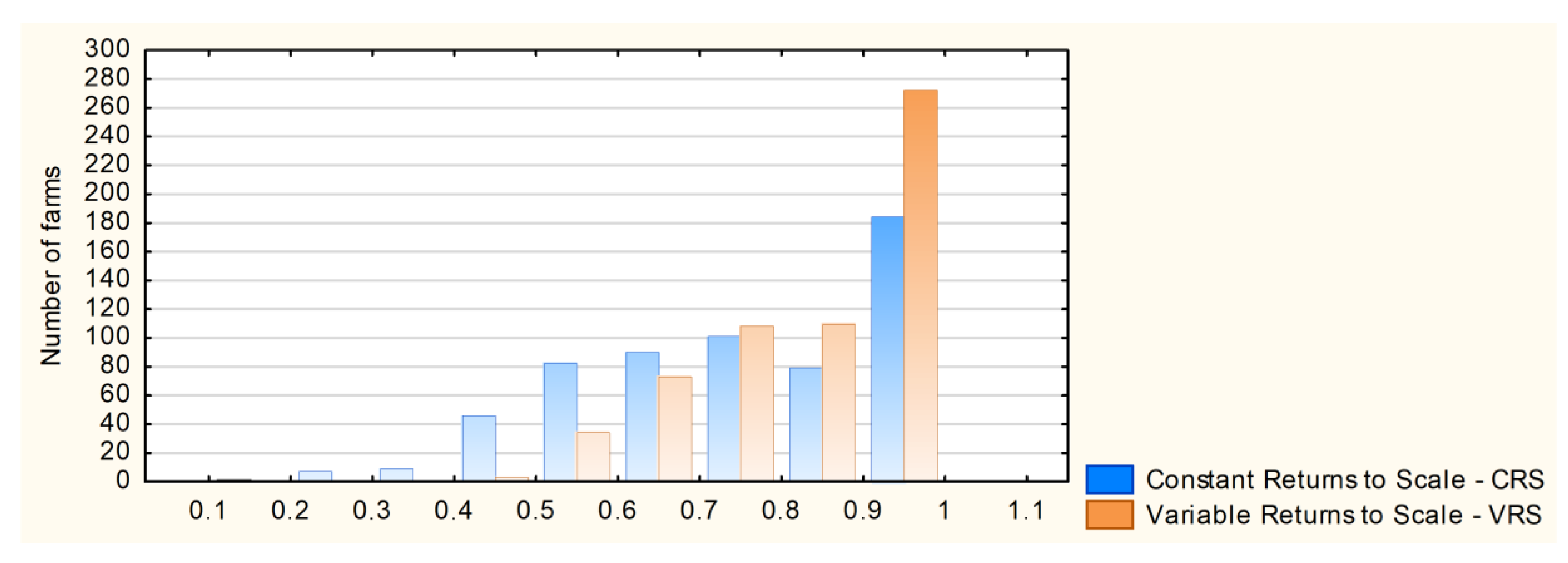2. Materials and Methods

2.1. Data Collection

The sample used for the analyses described in this paper consists of 601 farms participating in the Polish Farm Accountancy Data Network (FADN) system. The FADN sample in Poland covers 12,100 respondents that represent 730,000 farms exceeding 4000 EUR of standardized production. In the database detailed information concerning costs, production value, and financial results of the farms can be found, with the addition of basic facts describing the organization of work. The farms in the FADN database represents the most significant commercial farms. The FADN sample represents 93% of the total agricultural production in Poland, occupying an area of 85% of the agricultural land, keeping 97% of livestock, and provides employment for two thirds of people working in the Polish farm sector. In this paper, we used data coming not only from the FADN database, but also from direct structured interviews with farmers.

The 601 farms were selected using a layer/random selection procedure, which covered:

4 layers representing farm specialization

3 layers representing standard production size

4 layers representing administrative regions

To determine the number of farms in each layer, the Neyman [115] method was used, based on the methodology of determining the sample size for FADN [116]:

$${\mathrm{n}}_{\mathrm{h}}=\mathrm{n}\frac{N_h{\sigma }_h}{{{\displaystyle \sum }}_{k=1}^L{N}_k{\sigma }_k}$$

(1)

where:

n_h—sample size in layer h,

n—sample size,

N_h—the size of the population in layer h,

σ_h—standard deviation in layer h,

L—number of layers.

The methodology of two-phase sampling is presented in the statistical literature [117,118]. For each stratum, the number of farms to be surveyed was estimated with Neyman’s method (Equation (1)). The farms for interviews were then randomly selected from all FADN farms belonging to each stratum. In the case of farmers refusal, another farm from selected stratum was chosen. The applied methodology of selecting farms ensured that the structure of the sample reflects the structure of the entire FADN population (in terms of economic size, type of production, and region).

Carrying out the interviews (in 2017) was outsourced to advisers from regional extension centers, who usually coordinate the collection of data for the FADN database. The questionnaire contained questions on behavioral aspects of the operation of farms, including attitudes towards environmental and societal aspects of sustainability. The data obtained from questionnaires were added to data available in the FADN database (farm costs, production value, financial results, and basic organizational data).

2.2. Environmental Impact Operationalisation

Our DEA model is supposed to include traditional economic inputs, as well as the environmental impact of farming. To illustrate the negative environmental impact of farms, we decided to use the following indicators: nitrogen (N) and phosphorus (P) surpluses, as well as GHG emissions at the level of the farm. These parameters were chosen because farming is responsible for a large share of nitrogen and phosphorus flows to the biosphere and oceans, and GHG emissions, as was already written in the literature review. Other negative impacts of agriculture as biodiversity loss and deforestation were not analyzed because they result from the overall impact of the agricultural sector, and are difficult to assign or measure at the level of individual farms. The freshwater consumption, even though it could be assigned to a particular farm, was not analyzed as irrigation of crops is very marginal in Poland.

To estimate the GHG emissions and nutrients, a specific procedure to estimate environmental pressures base on FADN data has been applied [119,120]. Due to the limitations of the FADN dataset, which consists mainly of financial data, several assumptions were made. To estimate the volume of nutrients delivered and emissions from fertilizers, information from the FADN database on the amount of purchased fertilizers and expenditures on nitrogen, phosphorus, and compound fertilizers were used.

Estimation of the nutrient balance (N, P) was made based on the OECD methodology, taking into account soil as a system boundary [121]. Due to the adopted analysis variant (soil), the balance of nutrients was determined per area unit, indicating the excess of nitrogen [kg N/ha] and phosphorus [kg P₂O₅/ha] per hectare of UAA, respectively.

The following sources of nitrogen and phosphorus were included in the nutrient balance:

• nitrogen and phosphorus in mineral fertilizers (estimated based on FADN data)
• nitrogen and phosphorus in animal feces (the volume of mineral components from natural fertilizers was determined based on the average annual number of farm animals in each farm),
• nitrogen biologically bound by free-living bacteria and legumes (the amount of nitrogen obtained from natural sources (biological binding and atmospheric precipitation) was estimated, taking into account the dependence of biological nitrogen fixation processes on soil quality [122]; moreover, it was taken into account that the cultivation of legumes provides 60 kg N/ha [123].),
• nitrogen from precipitation [10 kg N/ha],
• nitrogen and phosphorus in the seed material.

To close the balance, the nitrogen and phosphorus carried out of the fields with the harvest were taken into account:

• commercial plants,
• fodder crops.

The amounts of nutrients taken out were determined based on the production volume of individual crops (FADN data) and the content of nitrogen and phosphorus in individual crops [124,125]. Data on the area of agricultural land, soil quality, and the structure of crops were obtained from the FADN data.

To determine GHG emissions from the farm sector, Intergovernmental Panel on Climate Change (IPCC) [126] guidelines and normative GHG emissions resulting from the use of energy carriers, were applied. Greenhouse gas emissions were calculated as CO₂ equivalents at farm level [kg CO_2eq] and per area unit [kg CO_2eq/ha]. When estimating GHG emissions from the agricultural sector using the IPCC methodology, the following emissions were taken into account:

• enteric fermentation emissions (equation IPCC 10.21, tier 1 & 2),
• direct and indirect emissions from manure management (equations IPCC 10.23, 10.25, 10.26, 10.28),
• direct and indirect emissions from managed soils (equations IPCC 11.1, 11.6, 11.9, 11.10, 11.11),
• emissions from urea and agricultural lime applications (equations IPCC 11.13, 11.12).

The GHG emission factors for individual activities were established, taking into account the production intensity level [119].

In addition to GHG emissions determined following the IPCC methodology for the agricultural sector, the GHG emissions resulting from the use of energy carriers in farms were taken into account. For this purpose, the expenditures of farms on energy carriers were converted into physical units using the average prices from 2017, and then for the obtained level of consumption, the GHG emission level was determined using emission factors, adopted based on literature sources [127,128,129].

In the next phase of the study, the estimated values of GHG emissions, and nitrogen and phosphorus surpluses, were treated as variables illustrating the environmental pressures generated by the farms.

2.3. Specification of DEA Models for Eco-Efficiency Evaluation

DEA as a non-parametric technic of efficiency assessment was proposed by Charens et al. [130]. During the analysis, the decision-making units (DMU) characterized by the best relations of inputs to outputs were marked with 1 and formed a frontier of efficiency; the remaining DMUs, that obtained score under 1, were evaluated in comparison to the best ones. The methodology of DEA did not provide any guidelines for selecting a particular number or type of input and output variables [131]. Usually, efficiency analyses in agriculture with DEA application involve variables reflecting resource consumptions as inputs, and a measure of production as output. Both inputs and outputs can be expressed in financial as well as in physical measures [132].

Usually, inputs contain such variables as agricultural land, labor, capital, and different categories of costs. In our research, we also implemented some variables that should reflect the environmental impact; they were operationalized as inputs, to reflect environmental cost (see also Pishgar-Komleh et al. [133], Manello [134], and Ramili and Munisamy [135] for a similar approach to including negative externalities in efficiency measurement).

The full set of variables used in the DEA model was as follows:

• x₁—utilized farm area in ha (land in ha),
• x₂—number of work units (AWU),
• x₃—value of assets (capital without land value),
• x₄—value of indirect consumption, including agricultural products from own production used for production purposes, as well as materials from purchase, energy, external services, and other costs related to production,
• x₅—nitrogen surpluses in kg N per farm (estimated on farm’s N balance),
• x₆—phosphorus surpluses in kg P₂O₅ per farm (estimated on farm’s P balance),
• y₁—output—value of the farm’s agricultural production.

The averages values of inputs (excluding variables reflecting environmental pressures which are described in Section 3) and output are presented in

Table 1. Average values of inputs and output.

Farms	Value of Assets (Capital) [Thousand EUR]	Utilized Farm Area in ha [Land in ha]	Number of Work Units [AWU]	Indirect Consumption [Thousand EUR]	Production [Thousand EUR]
Farm type
Cattle	142.3	29.8	1.81	24.8	42.3
Cereals	136.0	77.0	1.56	40.0	65.7
General Crop	104.9	45.5	2.18	30.9	55.7
Mixed	101.4	35.3	1.74	30.2	42.8
Others	147.3	9.0	2.68	38.7	76.1
Pigs	180.8	38.0	2.03	94.1	118.3
Total	130.3	40.5	1.89	38.3	59.1
Economic size (standard output in thousand EUR)
≥4; <25	54.4	15.8	1.48	9.9	15.0
≥25; <100	149.3	44.6	2.00	37.2	62.3
≥100	369.7	126.8	3.09	162.9	231.7

Annual Working Unit [2120 h]. Source: own elaboration.

.

Two separate DEA models were calculated: one with constant returns to scale (CRS) (Equation (2)) and one with variable returns to scale (VRS) (Equation (3)) [136]. A detailed description of how these models should be prepared can be found in a rich body of literature (i.e., Weaver [137], Weaverand Kim [138], Coopper et al. [139]). All models were inputs-oriented, which results from the fact that a farmer can decide mainly about inputs (controlled variables) whereas outputs are uncontrolled ones. The CRS model expresses overall technical efficiency, while the VRS model pure technical efficiency. Comparing the result of these two models allows assessing scale effects (SE) of a particular decision making unit (DMU).

Basic CRS version of the model can be described with the following formula:

$$\mathsf{\theta }=h_i(\mathsf{\mu },\mathsf{\upsilon })=\frac{{{\displaystyle \sum }}_{r=1}^R{\mu }_r{y}_{r_i}}{{{\displaystyle \sum }}_{p=1}^P{\upsilon }_p{x}_{p_i}}\to \max$$

(2)

where:

$$\frac{{{\displaystyle \sum }}_{r=1}^R{\mu }_r{y}_{r_i}}{{{\displaystyle \sum }}_{p=1}^P{\upsilon }_p{x}_{p_i}}\le 1,{\mu }_r\ge 0,v_p\ge 0$$

h_i—efficiency of DMU (i = 1,….,n)

μ_r—weights of outputs (r = 1,…..,R)

v_p—weights of inputs (p = 1,….,P)

y_ri—vector of outputs

x_pi—vector of outputs

The VRS version of the model can be described by:

$$\mathsf{\theta }=h_i(\mathsf{\mu },\mathsf{\upsilon })=\frac{{{\displaystyle \sum }}_{r=1}^R{\mu }_r{y}_{r_i}-u_o}{{{\displaystyle \sum }}_{p=1}^P{\upsilon }_p{x}_{p_i}}\to \max$$

(3)

where:

$$\frac{{{\displaystyle \sum }}_{r=1}^R{\mu }_r{y}_{r_i}}{{{\displaystyle \sum }}_{p=1}^P{\upsilon }_p{x}_{p_i}+u_0}\le 1,{\mu }_r\ge 0,v_p\ge 0$$

u_o—intercept of VRS model (vector of returns to scale)

The calculations were carried out with Efficiency Measurement System software by Scheel [140]. The calculations were carried out separately for each production type (cereals farms, general crops farms, cattle farms, pigs farm, mixed farms, others), as efficiency analysis with DEA method requires choosing a sample of DMU characterized with similar production technique.

2.4. Farm Sustainability Indicators and Other Assumptions

Eco-efficiency indicators evaluated with the use of DEA were further compared with a set of farm characteristics and sustainability indicators in economic, environmental, and social dimensions. The sustainability indicators were calculated in a multiphase procedure [141]. In the first stage, on the basis of data from the interview questionnaire and the FADN database, 51 diagnostic variables characterizing the environmental, economic, and social dimension of sustainability at the farm level were determined. These variables were then aggregated into seven sub-indices including indicators of:

• the correctness of agricultural practice in plant production,
• indicators of the correctness of agricultural practice in livestock production,
• environmental perception indicator,
• production potential indicator,
• economic potential indicator,
• indicator of living conditions,
• mental comfort indicator.

The first three were used to determine the aggregate sustainability index for the agro-environmental dimension, the other two for the economic dimension and the last two for the social dimension. The above mentioned indicators were further compared with the eco-efficiency indicators. A detailed description, including FADN variables and primary data, used for the construction of the indices can be found in earlier publications of the authors [142,143]. The sustainability indicators, and some other variables describing the farms, were analyzed to compare groups of farms characterized by different eco-efficiency levels. The sample was divided into four groups, using the quartile method, depending on the level of overall efficiency indicator.

3. Results

3.1. Environmental Pressure

To calculate the eco-efficiency of the farms, it was necessary to assess the environmental pressure of the farms. As was written above, nitrogen and phosphorus surpluses, as well as GHG emissions, were used. Estimated levels of these parameters per 1 ha of utilized agricultural area (UAA) are given in

Table 2. Nitrogen and phosphorus surpluses and greenhouse gas (GHG) emissions per 1 ha of agricultural land by farm type and economic size in the sample of Polish commercial farms.

Farms	N Surplus [kg/ha]	P2O5 Surplus [kg/ha]	GHG Emissions [kg CO2eq/ha]—Only Agricultural Sources	GHG Emissions [kg CO2eq/ha]—Agricultural Sources + Energy Carriers Use
Farm type
Cattle	64.8	11.4	4676.1	5057.7
Cereals	83.2	−13.1	1184.1	1500.3
General Crop	91.5	2.3	1334.4	1622.4
Mixed	97.3	7.9	2073.4	2393.7
Others	95.5	29.9	1517.5	9271.2
Pigs	166.1	127.0	3399.1	4053.5
Economic size (standard output in thousand EUR)
≥4; 25	72.7	3.6	1717.7	2017.5
≥25; <100	92.2	8.8	2708.9	3217.1
≥100	107.0	26.6	1963.4	2420.0
Total	93.7	13.8	2291.0	2746.0

Source: own research.

. On average, nitrogen and phosphorus surpluses reached 93.7 kg N/ha and almost 13.8 kg P₂O₅/ha of UAA.

Significantly high emissions of nitrogen and phosphorus were observed in pig farms, where a widely known problem of manure management exists, as those farms maintain relatively high production on a relatively small land. Similarly, GHG emission in this group was also visibly higher than the average. Nevertheless, GHG emissions were the highest in cattle farms, which is also a common issue resulting from the high enteric fermentation. However, after including energy carrier use, the highest total GHG emission per 1 ha was observed in farms described as “others”; this group includes, among other, specialized horticultural farms that use a lot of energy in the greenhouses (usually heating, which in Poland is in about three quarters based on coal). The lowest pressures were observed in the “cereals” type. This group was also characterized by negative phosphorus surplus, which nevertheless is not a positive outcome at a farm level, as in the future it will probably decrease the production potential of soil. When we look at the economic size of the farms, relatively lower emissions per 1 ha are observed in farms with smaller economic size.

Even though it seems reasonable to calculate nitrogen and phosphorus surpluses per 1 ha (as these substances leak directly to the soil), it seems less obvious to do so with GHG emissions. Thus the environmental pressures were calculated also per 1 EUR of agricultural production (

Table 3. Nitrogen and phosphorus surpluses and GHG emissions per 1 EUR of agricultural production by farm type and economic size in the sample of Polish commercial farms.

Farms	N Surplus [g/1 EUR]	P2O5 Surplus [g/1 EUR]	GHG Emissions [kg CO2eq/1 EUR]—Only Agricultural Sources	GHG Emissions [kg CO2eq/! EUR]—Agricultural Sources + Energy Carriers Use
Production type
Cattle	2.59	0.45	186.56	201.79
Cereals	5.69	−0.82	79.71	100.47
General Crop	4.23	0.10	61.72	75.04
Mixed	4.55	0.37	96.86	111.83
Others	1.15	0.36	18.24	111.42
Pigs	3.03	2.32	61.98	73.91
Economic size (standard output in thousand EUR)
≥4; <25	4.37	0.21	103.17	121.18
≥25; <100	3.75	0.36	110.05	130.69
≥100	3.32	0.83	60.91	75.07
Total	3.64	0.54	89.00	106.68

Source: own research.

). This indicator includes the relation between environmental pressures and economic effects, and thus could be perceived as an eco-efficiency measure. The results obtained, seen in Table 2 and Table 3, visibly differ. Concerning the production value, the highest nitrogen surplus was observed in crop farms (cereals and general crops) as well as mixed farms. The highest phosphorus emissions were observed in pig farms, as in the previous approach. When considering GHG emissions to production value, the highest negative impact was observed in cattle farms, twice as much as the average.

When we look at the economic size, nitrogen and GHG emissions per production unit are visibly lower in the largest farms, which suggests that they are the most efficient. This rule, however, does not refer to the phosphorus surplus, which is the highest in the largest farms. It might be a result of over-fertilization, because economically stronger farms have a greater possibility to use more fertilizers other than nitrogen in comparison to weaker ones.

3.2. Eco-Efficiency According to the DEA Method

Even though the above presented data provide us with interesting knowledge concerning the environmental pressure generated by various farm types, they do not give precise answers to the question of which farm types are more, and which less, harmful to the natural environment (in fact, all of them create adverse effects but exact emissions vary depending on farm type and emission type). The use of DEA allowed for aggregating all of the analysis elements and giving the answer in the form of a single indicator.

The distribution of both eco-efficiency indicators (CRS and VRS) for the whole sample are presented on Figure 1, while

Table 4. Average eco-efficiency indicators calculated with the data envelopment analysis (DEA) method, depending on production type and economic size classes, and the share of fully efficient farms in the sample of Polish commercial farms.

Farms	Eco-Efficiency Indicators			Conventional Efficiency Indicators			% of Fully Efficient Farms
	CRS	VRS	SE	CRS	VRS	SE
Production type
Mixed	0.77	0.83	0.85	0.69	0.77	0.89	36.6
Cattle	0.78	0.86	0.88	0.60	0.78	0.76	29.3
Cereals	0.74	0.88	0.83	0.69	0.85	0.81	39.2
Pigs	0.77	0.84	0.84	0.73	0.84	0.87	25.8
Others	0.69	0.85	0.82	0.60	0.80	0.74	41.3
General Crop	0.73	0.86	0.84	0.66	0.81	0.81	41.1
Economic size (standard output in thousand EUR)
Small	0.70	0.85	0.84	0.57	0.79	0.72	32.0
Medium	0.79	0.84	0.85	0.71	0.80	0.89	36.5
Large	0.85	0.89	0.87	0.82	0.86	0.95	41.3
Total	0.76	0.85	0.85	0.66	0.80	0.82	34.9

CRS—Constant Return to Scale, VRS—Variable Return to Scale, SE—Scale Efficiency. Source: own research.

contains information regarding average eco-efficiency indicators, and a share of fully efficient farms regarding production type and economic size class. It is worth remembering that DEA efficiency indicators are relative ones, taking values in the range from 0 to 1. The distance between a particular DMU and a fully efficient one (calculated as the difference between this DMU indicator and 1) shows a possible range of improvement.

In the whole sample, on average only just under 35% of DMUs were fully efficient, which means that about 65% of farms should reduce the volume of inputs used. Average eco-efficiency indicator in the CRS model reached 0.76. This means that an average farm could reduce its production inputs and environmental pressure by almost one quarter without reducing its production effects. Average differences between production types were rather small, relatively the most effective on average were cattle farms, while the least effective were “other” (although in this group the highest share of fully effective farms was observed). Economic size seems more important for the efficiency, the lowest indicator was found in the smallest farms, while the highest in the largest.

However, we should be aware of the fact that the constant return to scale assumption is appropriate only if the scale of production is optimal. In changeable farming conditions, it is good to check also pure technical efficiency (VRS model), as it analyses the way of converting inputs into outputs, ignoring the effect of production scale. On average, the VRS efficiency indicator reached 0.85 and only slightly differed regarding the economic size of the farm (again, the most effective were the largest farms, in economic terms, and the largest farms group contained the largest share of fully efficient farms). Taking into account the criterion of the production type, we can observe that on average the differences in pure technical eco-efficiency scores between farm groups are rather small; cereals farms turned out to be the most efficient in this case. This may seem understandable, given their negative phosphorus balance and the lowest level of GHG emission per hectare (however, it should be borne in mind that the indicators were calculated separately for individual production types, so direct comparisons are of limited analytical importance). The observed higher level of differentiation of the CRS indicators than the VRS may be related to the fact that it is a more complex measure, which includes both pure technical efficiency as well as scale efficiency. Some farms may efficiently convert inputs into outputs but do not operate at optimal scale, while others may have efficient technology (or not) and also operate at optimum scale. As a result, the CRS indicator covering these two aspects may naturally be more diverse than the VRS focusing on only one dimension.

Observed differences between eco-efficiency scores in CRS (constant return to scale) and VRS (variable returns to scale) show that the scale of production is inefficient; if it was efficient, both CRS and VRS indicators would reach 1. The highest differences between considered indicators are in the smallest farms. On average, the SE scores were close to the VRS level, which means that the overall technical inefficiency was determined equally by the method of inputs converting into outputs (pure technical efficiency) and by their production scale.

Including variables reflecting environmental impact in the analysis translates into an increase in the average efficiency indicators. However, this fact should not be associated with an absolute improvement in efficiency, but with a downshift of the efficiency frontier (which is an obvious consequence of introducing additional inputs into the calculation). The shift of the efficiency frontier occurs as a result of the deterioration of the absolute relations of effects to inputs for the DMU creating frontier. As a result of this process, the frontier becomes closer to some of the remaining units (previously strongly ineffective), which translates into a higher average efficiency indicators level. The inclusion of environmental variables, therefore, influences a more “fair” classification of farms, although it should be emphasized that objects that were effective in the “conventional” approach remained effective also in “eco-efficiency” models.

3.3. Characteristics of Farms in Various Eco-Efficiency Groups

To better understand differences in eco-efficiency between the farms, additional analyses of farms, depending on their eco-efficiency level, were carried out. The sample was divided according to the CSR level (that is the level of technical efficiency, combining pure technical efficiency and the effects of scale).

Table 5. Farm characteristics according to the eco-efficiency groups (gr. I, the lowest eco-efficiency, gr. IV, the highest eco-efficiency) of Polish commercial farms.

Farm Characteristics		Eco-Efficiency Group					Differences Significance
		Gr. I	Gr. II	Gr. III	Gr. IV	Total Sample	F-Test	p-Value
utilized agricultural area (UAA) [ha]		23.6	37.7	47.6	53.7	40.6	8.379	0.0000
livestock [LU]		11.2	29.2	41.1	37.0	29.6	8.542	0.0000
Value of capital per farm [thousand EUR]		170.3	265.2	353.1	366.8	288.5	12.297	0.0000
Indebtedness indicator (borrowed capital/assets) [%]		4.2	5.1	11.2	11.4	8.8	6.177	0.0004
Production value	thousand EUR per farm	20.1	47.9	71.8	97.5	59.2	17.72	0.0000
	thousand EUR per 1 ha of UAA	0.9	1.3	1.5	1.8	1.5	3.791	0.0103
Farm income	thousand EUR per farm	4.3	11.3	22.8	34.9	18.3	33.014	0.0000
	thousand EUR per 1 ha of UAA	0.18	0.3	0.48	0.65	0.5	3.625	0.0129
	related to the production value (production profitability)	0.21	0.24	0.32	0.36	0.3	11.32	0.0000
Total cost of chemical fertilizers, pesticides, and fungicides in relation to the production value		0.2	0.19	0.16	0.14	0.2	7.598	0.0001

Source: own research.

contains a set of production potential elements, depending on the farm efficiency level. Eco-efficiency groups were obtained through dividing the sample into four quartiles (group I includes one quarter of the sample with the lowest score of eco-efficiency indicator, while group IV meant one quarter of the sample with the highest score of eco-efficiency indicator). As the table shows, there are visible differences between the eco-efficiency groups concerning almost all chosen parameters.

The most efficient farms (group IV), in comparison to the rest of the sample, were on average visibly larger in terms of area, and had more valuable assets (but simultaneously they were more indebted than the rest of the sample). We could also notice that the higher eco-efficiency of the farms is, the higher production value is. Of course, this could be the result of the farm size, but income in both absolute and relative terms was also growing with the eco-efficiency growth. It is worth also noting that production profitability (measured as the relation of farm income to the production value) was constantly rising with the rise of eco-efficiency. At the same time, total costs of chemical fertilizers, pesticides, and fungicides in relation to the production value are dropping with the rise of eco-efficiency. This is an interesting fact that could be raised in the discussion on the usefulness of “sustainable intensification”. All the differences were statistically significant (ANOVA F-test value and p-values are presented in Table 5).

In addition to basic farm characteristics, a comparison of farm sustainability levels depending on the eco-efficiency group was prepared. The sustainability indicators were related according to the procedure presented in the methods section.

Table 6. Sustainability indicators of Polish commercial farms according to the eco-efficiency groups (gr. I, the lowest eco-efficiency, gr. IV, the highest eco-efficiency).

Sustainability Indicators		Eco-Efficiency Group					Differences Significance
		Gr. I	Gr. II	Gr. III	Gr. IV	Total Sample	F-Test	p-Value
Agro-environmental dimension	Indicator of the correctness of agricultural practice in plant production	0.48	0.51	0.51	0.54	0.51	2.66	0.0475
	Indicator of the correctness of practice in livestock production*	0.59	0.60	0.62	0.63	0.61	1.75	0.1559
	Environmental perception indicator	0.64	0.67	0.68	0.68	0.67	1.18	0.3180
	Aggregated indicator	0.57	0.60	0.60	0.62	0.60	2.95	0.0321
Economic and production dimension	Economic potential indicator	0.36	0.50	0.59	0.61	0.51	40.56	0.0000
	Production potential indicator	0.46	0.52	0.52	0.53	0.50	4.72	0.0029
	Aggregated indicator	0.41	0.51	0.55	0.57	0.51	62.23	0.0000
Social dimension	Indicator of living conditions	0.59	0.61	0.62	0.63	0.61	1.43	0.2338
	Mental comfort indicator	0.51	0.53	0.55	0.55	0.53	4.38	0.0046
	Aggregated indicator	0.55	0.57	0.58	0.59	0.57	4.24	0.0056
Sustainability indicator		0.51	0.56	0.58	0.59	0.56	35.55	0.0000

* included in the aggregate indicators only for farms with animals. Source: own research.

shows that the average values of most of the sustainability indicators slightly rise with the rise of the eco-efficiency level (the differences in the levels of the environmental perception indicator and the indicator of living conditions were statistically insignificant).

It is worth noting that the environmental perception indicator reached the highest score of all the sustainability indicators (0.67), but it did not differ depending on the eco-efficiency. This result suggests that most of the farmers are aware of the environmental problems regardless of their level of eco-efficiency. The living conditions indicator did not differ significantly, and its scores (0.61) were higher than the total sustainability indicator (0.56). It is also worth noting that the specified groups of farms differed significantly by the level of “mental comfort indicator”, which means that farmers from eco-efficient farms not only present better production and economic results, but also feel less stress and have more free time (however on average the differences are not huge).

4. Discussion and Conclusions

The problem of efficiency is one of the key issues discussed in mainstream economics [144]. Nevertheless, classical economics largely ignores the fact that production processes are followed by negative externalities, mentioned by Pigou [61] and later by Kapp [145], as well as Buchanan and Stubblebine [64].

It is worth noting, however, that a producer who externalizes a part of the enterprise’s costs gains a significant competitive advantage over producers that refrain from such actions. Thus, it is important to include in the efficiency assessment a set of variables that represent the “consumption” of the natural environment. This requirement is fulfilled by the eco-efficiency concept created in the 1990s. According to Daly [85] efficiency assessment requires considering the relations of man-made capital to joint consumption of natural resources. Following this advice, in this paper, the general eco-efficiency of farms was assessed with the use of the DEA method

This paper contains the assessment of eco-efficiency of various farm types, based on the representative sample of Polish commercial farms; the results were later compared with basic farm characteristics and a set of farm sustainability indicators. Until now, there were very few scientific publications devoted to analyzing the determinants of eco-efficiency [75,97,146,147]. To the best knowledge of the authors, there were no publications directly analyzing relations between eco-efficiency levels and aggregated sustainability indicators.

Undoubtedly, eco-efficiency is supposed to help in assessing the sustainability of certain units [12,16,148], but it refers to only some sustainability aspects (related to production and economic dimensions). Thus, comparing eco-efficiency levels with a set of sustainability indicators provides the reader with broader knowledge. Such a broader view is important, because, according to Picazo-Tadeo et al. [97], the potential high eco-efficiency of farms does not necessarily mean their high sustainability. Eco-efficiency assessment with the DEA method allows only for comparisons among a set of farms, in relative terms. On the other hand, sustainability should be understood in absolute terms, and even high eco-efficiency (understood as a relation of environmental pressure to the outputs) does not guarantee that the natural system tolerances are not violated.

In general, farms that are larger in terms of economic size are characterized by a higher production intensity (measured by the value of fertilizers and pesticides used per hectare), and at the same time by lower negative environmental impact per unit of production, which supports the idea of implementing sustainable intensification [108,109]. However, when we consider nitrogen, phosphorus, and GHG emissions per ha, smaller (in terms of production) farms create less environmental pressure. Thus, it seems that the interpretation of the results is partly dependent on the perspective adopted. When considering production types, cattle and pig farms create the highest environmental pressures, which illustrates a widely known problem with manure management [149,150,151]. In general, the results show that higher eco-efficiency is observed in economically larger farms, characterized by a higher production intensity per ha.

We could compare these results with those obtained by Passel et al. [152], who showed that, in general, larger farms have a higher level of sustainable efficiency. Research carried out by Berre et al. [153] revealed that most eco-efficient farms appear to be intensive systems. According to Ullah et al. [146], eco-efficiency of small and large farms (measured by farm area) did not differ significantly per production unit. Gomez-Limon et al. [75] found that the level of eco-efficiency of various cultivation systems depends on the soil-climate conditions what is a determinant of land productivity. Anyway, they underline that in line with the previous literature, their results “do not seem to shed much light on the determinants of eco-efficiency either” [75] (p. 405).

According to our analyses, more eco-efficient farms are characterized by larger UAA area, higher production value, and higher intensity of chemical inputs (fertilizers, pesticides, and fungicides) per 1 ha, but at the same time the amount of inputs used is lower per production unit. It is also worth noting that more eco-efficient farms achieved higher farm incomes in many terms; totally, per 1 ha of UAA, and per 1 EUR of production value (higher profitability). Thus, we can conclude that eco-efficient farmers are probably more modern (economically effective, they are not afraid to take credit, maybe they also fertilize more consciously) a bit out of concern for the environment, a bit out of knowledge, a bit to economize. This suggests that economic goals can be achieved simultaneously with environmental goals, provided that agricultural production is not wasted in the next stages (sales, processing, consumption). A similar remark was given by Mouron et al. [154] who, while analyzing eco-efficiency of a fruit farm, concluded that the rise of incomes does not necessarily mean higher environmental pressure (impacts such as ecotoxicity, eutrophication, and non-renewable energy use did not necessarily increase when farms increased their income). Other research also confirmed that eco-efficiency, thanks to cost savings, can have a positive impact on farm incomes [155,156]. On the other hand, Ullah et al. [146] (p. 1) remarked that “most farms cannot combine high economic performance and low environmental impacts”. Their empirical observation leads to the conclusion that small farms achieved higher eco-efficiency and “that under current technology, farmers’ objectives and practices there is little room to improve together with all aspects of sustainability with no trade-offs” [146] (p. 9).

The results of our research seem to be more optimistic. The analysis of the sustainability indicators shows that the largest differences between farms representing differing levels of eco-efficiency were observed in the economic dimension of sustainability; eco-efficient farms were characterized by higher levels of such sustainability indicators, such as the economic potential indicator and production potential indicator. The remaining indicators either did not differ significantly (environmental perception indicator and indicator of living conditions) or the differences were significant but small.

In general, we can conclude that farms characterized by higher eco-efficiency are more sustainable. Usually, these are farms that are economically stronger than the average and characterized by higher production levels. Farmers who decide to produce on a large scale may pay more attention to input costs and amounts used. Economically smaller farms generate fewer emissions per 1 ha, but greater per production unit, which reflects their lower productivity.

The policymakers, while designing a farm support system (and thus stimulating certain actions and decisions) should take into account economic, social, and environmental goals. It seems that in regions with high production potential, supporting more intense production, and keeping the eco-efficiency rules should be considered. On the other hand, in regions characterized with lower production potential, it might be valuable to support other (social-environmental) functions of agriculture, purposefully resigning from maximizing production itself and thus give less attention to efficiency.