
Exploring Neural Mechanisms of Reward Processing Using Coupled Matrix Tensor Factorization: A Simultaneous EEG–fMRI Investigation


Abstract
:1. Introduction
2. Materials and Methods
2.1. Subjects
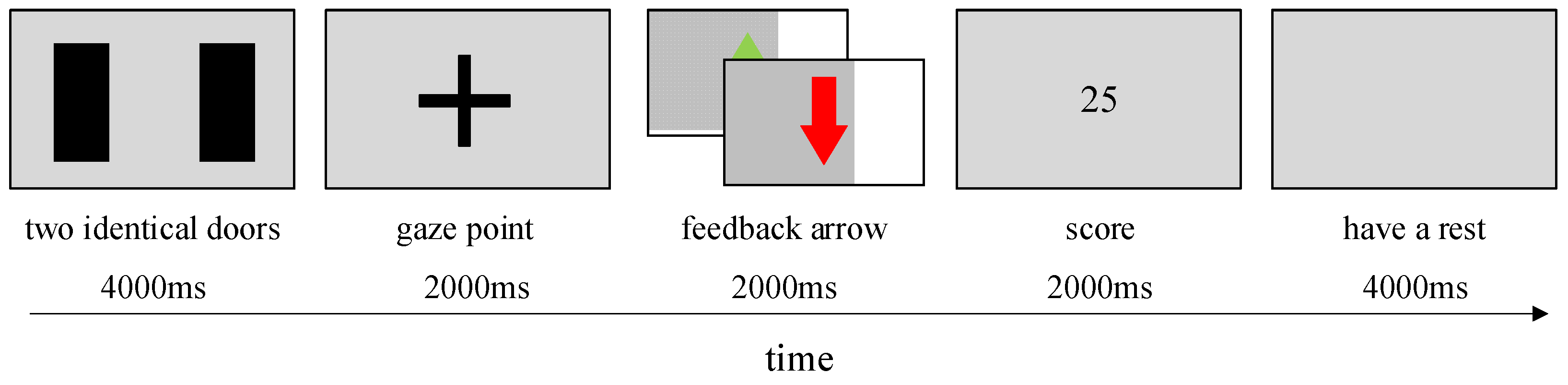
2.2. Gambling Task
2.3. Data Acquisition
2.4. Data Preprocessing
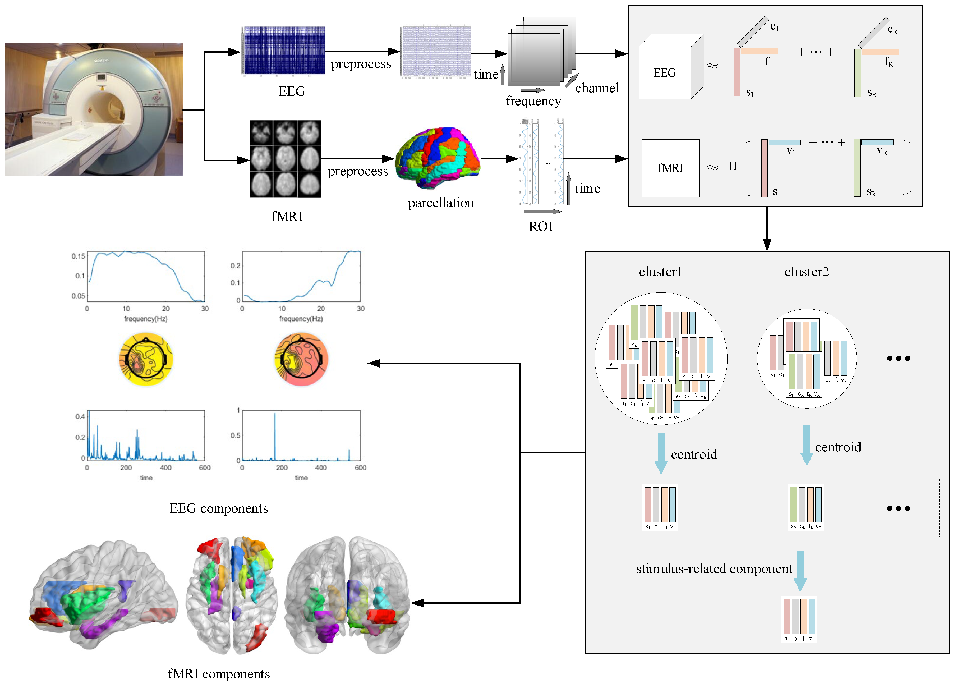
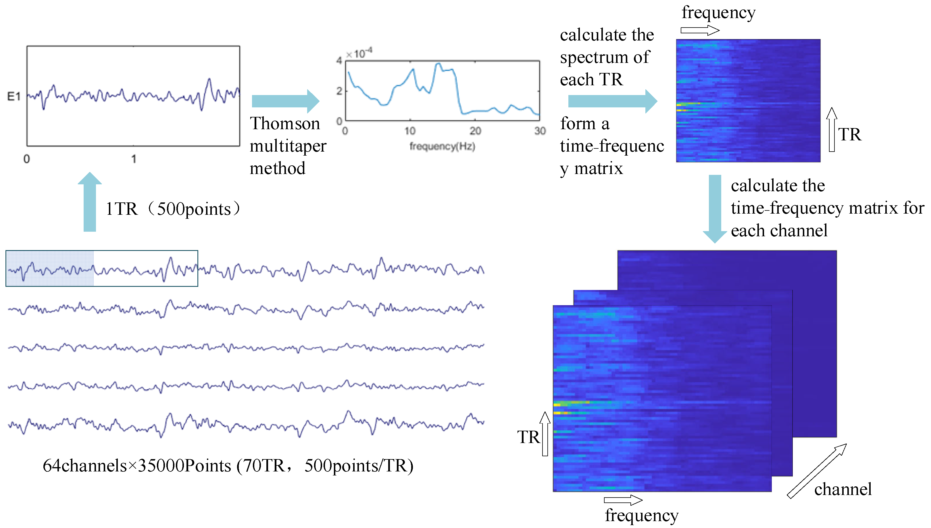
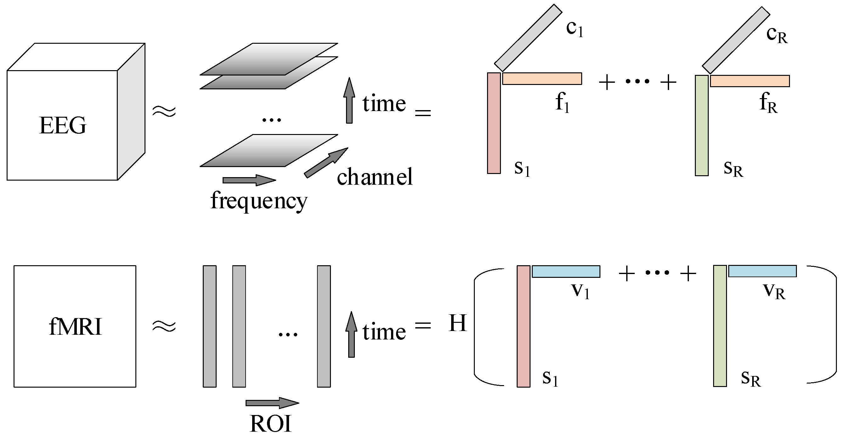
2.5. Higher-Order Data Representation
2.6. Modeling the Hemodynamic Response Function
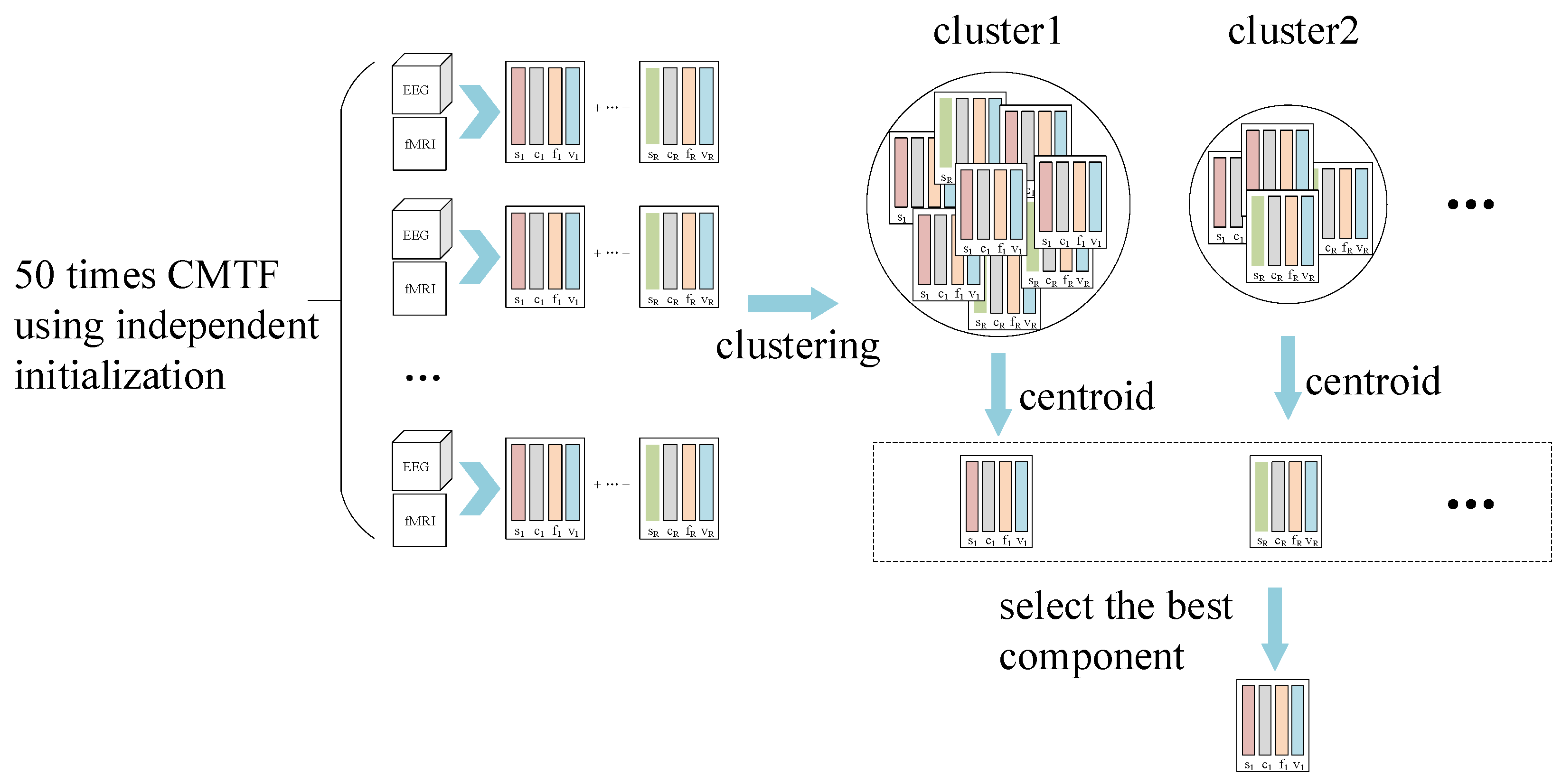
2.7. Coupled Matrix Tensor Factorization
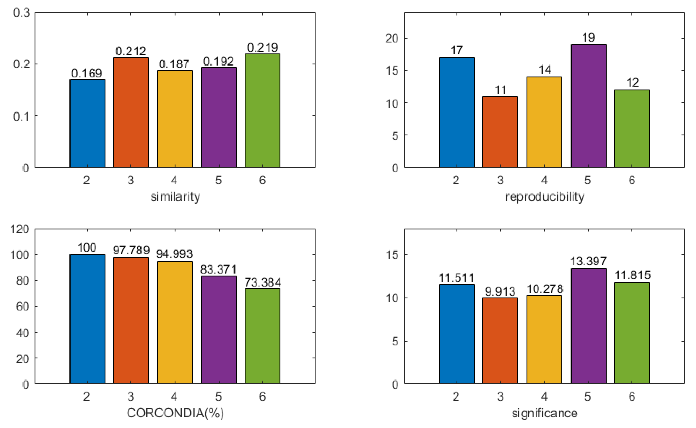
2.8. Model Selection
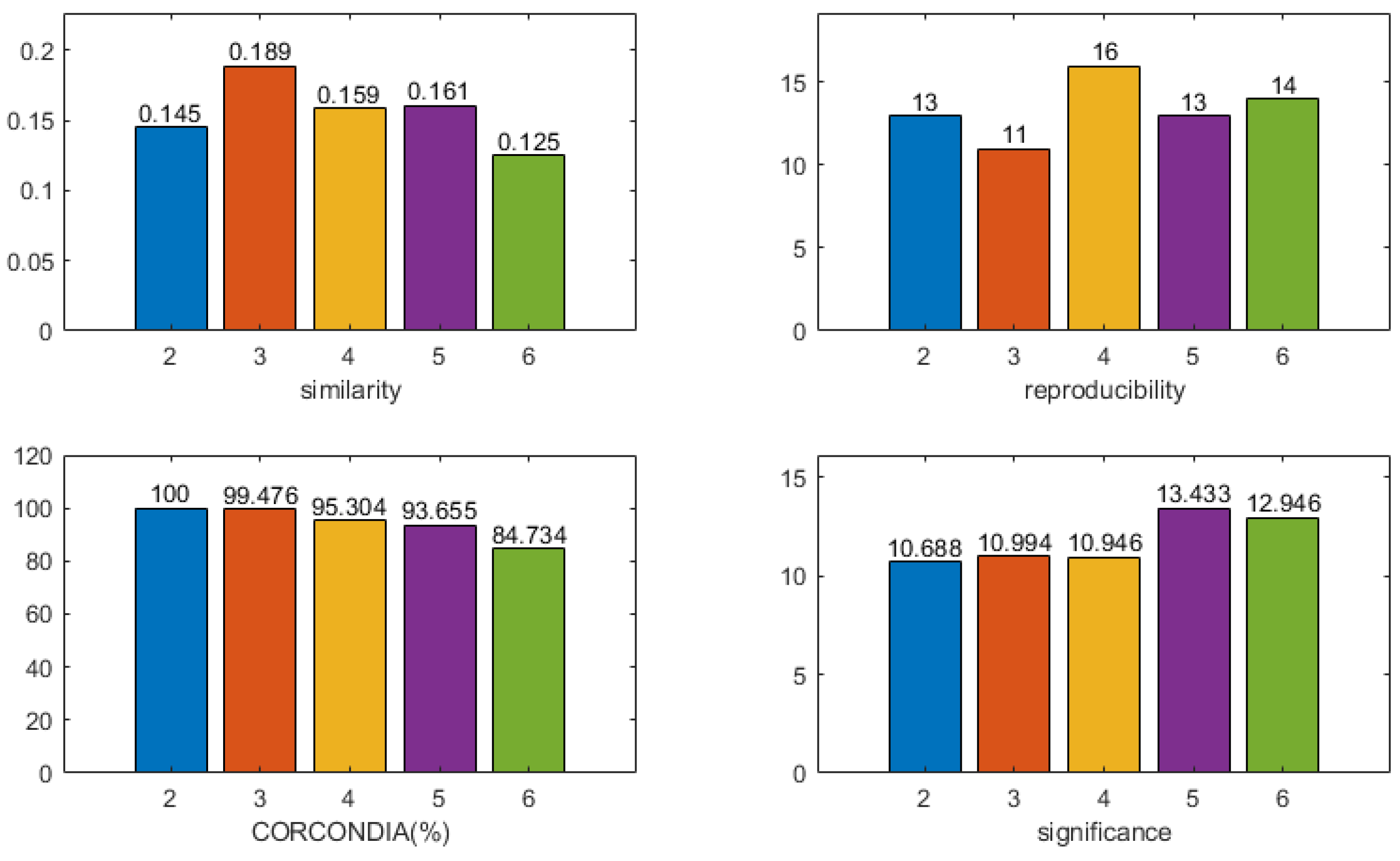
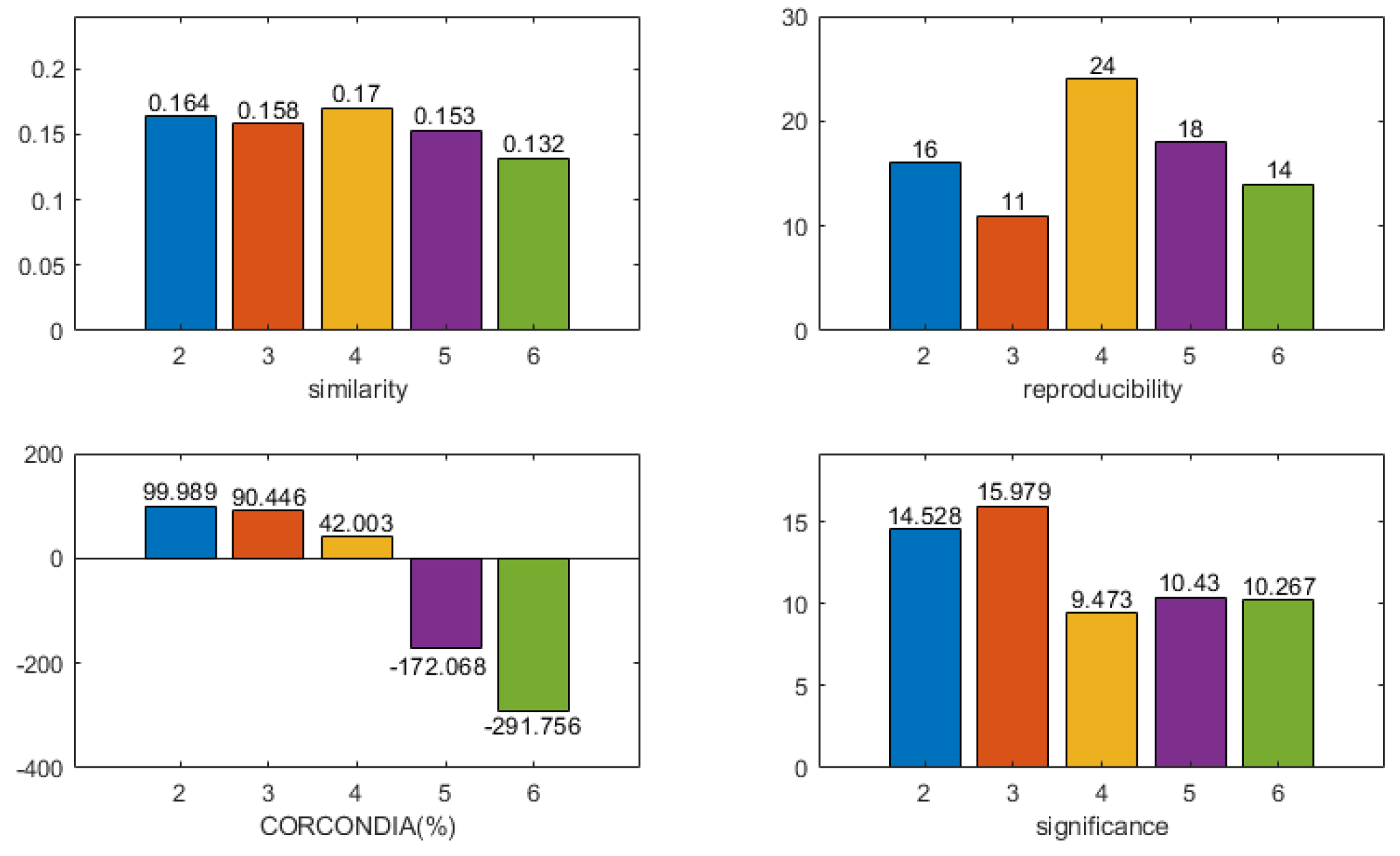
- CORCONDIA [50]: the CORCONDIA is computed for the EEG tensor in combination with EEG components , which describes how well the CP decomposition of a given number of components is appropriate for a given tensor and a given factor. Furthermore, 100% indicates an adequate model, and below 80% indicates an inappropriate model;
- Reproducibility of components: the cardinality of the component most relevant to the time course of the stimulus is calculated, and clusters of components with cardinality greater than 10 are retained;
- Similarity to the time course of the stimulus: the time course of the paradigm stimulus is constructed. If a stimulus (losing/winning) is available at a time point, it is 1. Otherwise, it is 0. The correlation between the time component and the time course of the paradigm stimulus is calculated, and the higher the correlation, the better the model fits;
- Significance of spatial components: a statistical non-parametric map (SnPM) is calculated based on the spatial signature . The familywise error (FWE) rate is controlled by setting the significance threshold at = 0.05. A higher statistical score indicates that the model is more suitable for the component.
3. Results
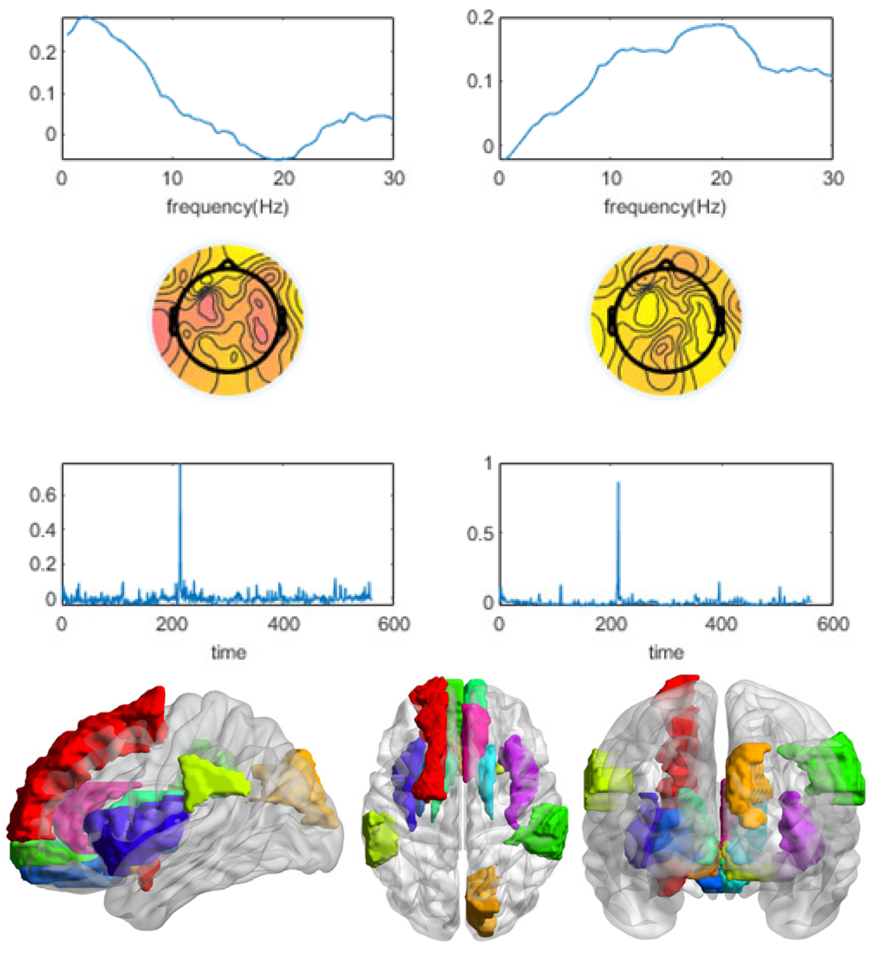
3.1. Winning and Losing Stimuli
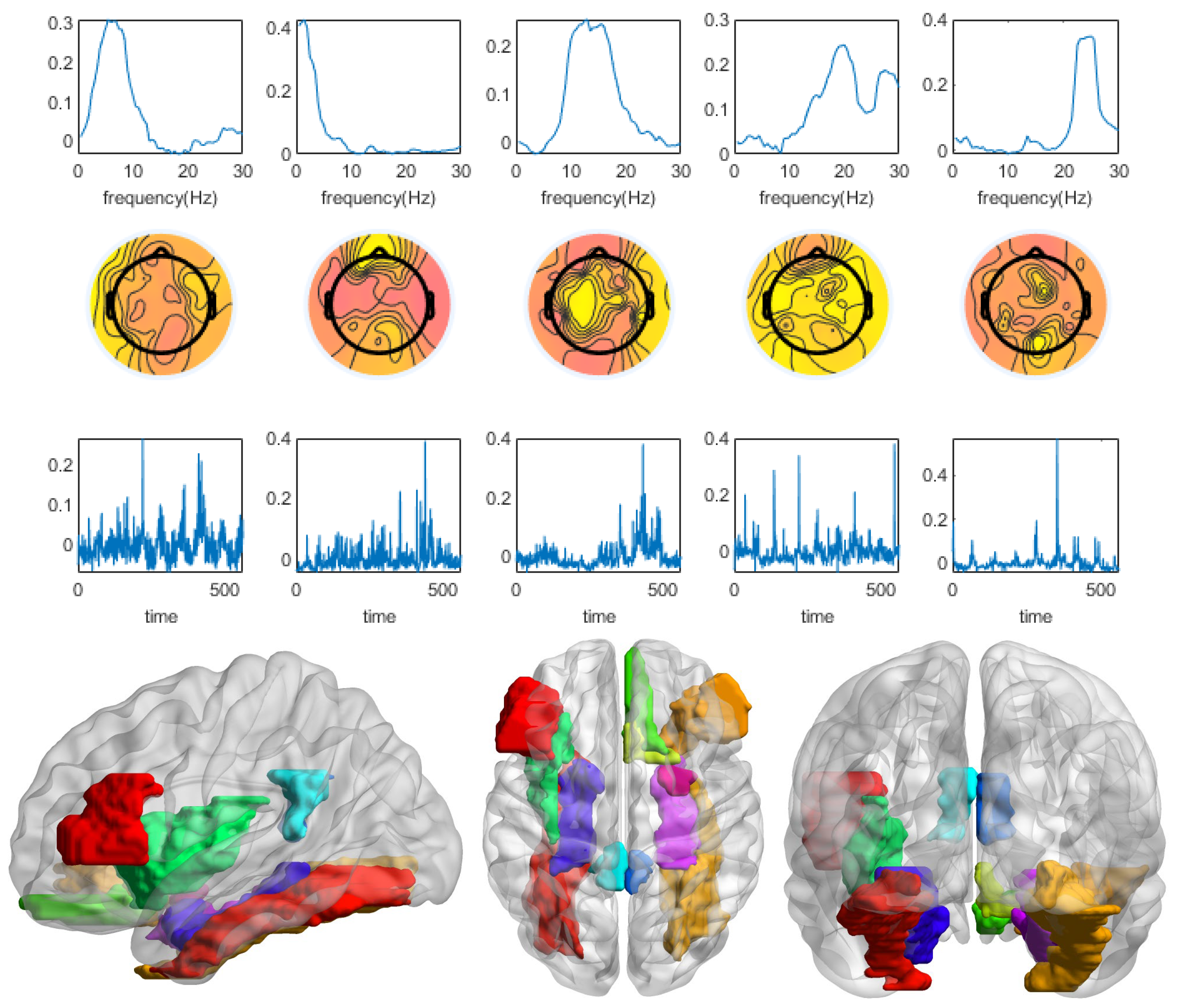
3.2. Winning Stimulus
3.3. Losing Stimulus
4. Discussion
5. Conclusions
Author Contributions
Funding
Institutional Review Board Statement
Informed Consent Statement
Data Availability Statement
Conflicts of Interest
References
- Gehring, W.J.; Goss, B.; Coles, M.G.H.; Meyer, D.E.; Donchin, E. The Error-Related Negativity. Perspect. Psychol. Sci. 2018, 13, 200–204. [Google Scholar] [CrossRef] [PubMed]
- Ng, T.H.; Alloy, L.B.; Smith, D.V. Meta-Analysis of Reward Processing in Major Depressive Disorder Reveals Distinct Abnormalities within the Reward Circuit. Transl. Psychiatry 2019, 9, 293. [Google Scholar] [CrossRef] [PubMed] [Green Version]
- Yang, D.-Y.; Chi, M.H.; Chu, C.-L.; Lin, C.-Y.; Hsu, S.-E.; Chen, K.C.; Lee, I.H.; Chen, P.S.; Yang, Y.K. Orbitofrontal Dysfunction during the Reward Process in Adults with ADHD: An FMRI Study. Clin. Neurophysiol. 2019, 130, 627–633. [Google Scholar] [CrossRef] [PubMed]
- Meyer, G.M.; Marco-Pallarés, J.; Boulinguez, P.; Sescousse, G. Electrophysiological Underpinnings of Reward Processing: Are We Exploiting the Full Potential of EEG? NeuroImage 2021, 242, 118478. [Google Scholar] [CrossRef]
- He, B.; Sohrabpour, A.; Brown, E.; Liu, Z. Electrophysiological Source Imaging: A Noninvasive Window to Brain Dynamics. Annu. Rev. Biomed. Eng. 2018, 20, 171–196. [Google Scholar] [CrossRef] [Green Version]
- Foti, D.; Weinberg, A. Reward and Feedback Processing: State of the Field, Best Practices, and Future Directions. Int. J. Psychophysiol. 2018, 132, 171–174. [Google Scholar] [CrossRef]
- Glazer, J.E.; Kelley, N.J.; Pornpattananangkul, N.; Mittal, V.A.; Nusslock, R. Beyond the FRN: Broadening the Time-Course of EEG and ERP Components Implicated in Reward Processing. Int. J. Psychophysiol. 2018, 132, 184–202. [Google Scholar] [CrossRef]
- Sambrook, T.D.; Goslin, J. Principal Components Analysis of Reward Prediction Errors in a Reinforcement Learning Task. NeuroImage 2016, 124, 276–286. [Google Scholar] [CrossRef] [Green Version]
- Jauhar, S.; Fortea, L.; Solanes, A.; Albajes-Eizagirre, A.; McKenna, P.J.; Radua, J. Brain Activations Associated with Anticipation and Delivery of Monetary Reward: A Systematic Review and Meta-Analysis of FMRI Studies. PLoS ONE 2021, 16, e0255292. [Google Scholar] [CrossRef]
- Elliott, R.; Friston, K.J.; Dolan, R.J. Dissociable Neural Responses in Human Reward Systems. J. Neurosci. 2000, 20, 6159–6165. [Google Scholar] [CrossRef] [Green Version]
- Dong, G.; Li, H.; Wang, Y.; Potenza, M.N. Individual Differences in Self-Reported Reward-Approach Tendencies Relate to Resting-State and Reward-Task-Based FMRI Measures. Int. J. Psychophysiol. 2018, 128, 31–39. [Google Scholar] [CrossRef]
- Cociu, B.A.; Das, S.; Billeci, L.; Jamal, W.; Maharatna, K.; Calderoni, S.; Narzisi, A.; Muratori, F. Multimodal Functional and Structural Brain Connectivity Analysis in Autism: A Preliminary Integrated Approach With EEG, FMRI, and DTI. IEEE Trans. Cogn. Dev. Syst. 2018, 10, 213–226. [Google Scholar] [CrossRef] [Green Version]
- Warbrick, T. Simultaneous EEG-FMRI: What Have We Learned and What Does the Future Hold? Sensors 2022, 22, 2262. [Google Scholar] [CrossRef]
- Zhu, Z.; He, X.; Qi, G.; Li, Y.; Cong, B.; Liu, Y. Brain Tumor Segmentation Based on the Fusion of Deep Semantics and Edge Information in Multimodal MRI. Inf. Fusion 2023, 91, 376–387. [Google Scholar] [CrossRef]
- Nguyen, T.; Potter, T.; Grossman, R.; Zhang, Y. Characterization of Dynamic Changes of Current Source Localization Based on Spatiotemporal FMRI Constrained EEG Source Imaging. J. Neural Eng. 2018, 15, 036017. [Google Scholar] [CrossRef]
- Li, W.; Zhang, W.; Jiang, Z.; Zhou, T.; Xu, S.; Zou, L. Source Localization and Functional Network Analysis in Emotion Cognitive Reappraisal with EEG-FMRI Integration. Front. Hum. Neurosci. 2022, 16, 960784. [Google Scholar] [CrossRef]
- Fang, F.; Houston, M.; Walker, S.; Nguyen, T.; Potter, T.; Zhang, Y. Underlying Modulators of Frontal Global Field Potentials in Emotion Regulation: An EEG-Informed FMRI Study. In Proceedings of the 2019 9th International IEEE/EMBS Conference on Neural Engineering (NER), San Francisco, CA, USA, 20–23 March 2019; IEEE: San Francisco, CA, USA, 2019; pp. 949–952. [Google Scholar]
- Adali, T.; Akhonda, M.A.B.S.; Calhoun, V.D. ICA and IVA for Data Fusion: An Overview and a New Approach Based on Disjoint Subspaces. IEEE Sens. Lett. 2019, 3, 7100404. [Google Scholar] [CrossRef]
- Hinault, T.; Larcher, K.; Zazubovits, N.; Gotman, J.; Dagher, A. Spatio–Temporal Patterns of Cognitive Control Revealed with Simultaneous Electroencephalography and Functional Magnetic Resonance Imaging. Hum. Brain Mapp. 2019, 40, 80–97. [Google Scholar] [CrossRef] [Green Version]
- Qin, Y.; Jiang, S.; Zhang, Q.; Dong, L.; Jia, X.; He, H.; Yao, Y.; Yang, H.; Zhang, T.; Luo, C.; et al. Ballistocardiogram Artifact Removal in Simultaneous EEG-FMRI Using Generative Adversarial Network. NeuroImage Clin. 2019, 22, 101759. [Google Scholar] [CrossRef]
- Keinänen, T.; Rytky, S.; Korhonen, V.; Huotari, N.; Nikkinen, J.; Tervonen, O.; Palva, J.M.; Kiviniemi, V. Fluctuations of the EEG-FMRI Correlation Reflect Intrinsic Strength of Functional Connectivity in Default Mode Network. J. Neuro Res. 2018, 96, 1689–1698. [Google Scholar] [CrossRef]
- Dehghani, A.; Soltanian-Zadeh, H.; Hossein-Zadeh, G.-A. Probing FMRI Brain Connectivity and Activity Changes during Emotion Regulation by EEG Neurofeedback. Front. Hum. Neurosci. 2023, 16, 988890. [Google Scholar] [CrossRef] [PubMed]
- Guo, Q.; Zhou, T.; Li, W.; Dong, L.; Wang, S.; Zou, L. Single-Trial EEG-Informed FMRI Analysis of Emotional Decision Problems in Hot Executive Function. Brain Behav. 2017, 7, e00728. [Google Scholar] [CrossRef] [PubMed]
- Hunyadi, B.; Dupont, P.; van Paesschen, W.; van Huffel, S. Tensor Decompositions and Data Fusion in Epileptic Electroencephalography and Functional Magnetic Resonance Imaging Data: Tensors in EEG-FMRI. WIREs Data Min. Knowl. Discov. 2017, 7, e1197. [Google Scholar] [CrossRef] [Green Version]
- Chatzichristos, C.; Kofidis, E.; van Paesschen, W.; de Lathauwer, L.; Theodoridis, S.; van Huffel, S. Early Soft and Flexible Fusion of Electroencephalography and Functional Magnetic Resonance Imaging via Double Coupled Matrix Tensor Factorization for Multisubject Group Analysis. Hum. Brain Mapp. 2022, 43, 1231–1255. [Google Scholar] [CrossRef]
- Chatzichristos, C.; Vandecapelle, M.; Kofidis, E.; Theodoridis, S.; Lathauwer, L.D.; van Huffel, S. Tensor-Based Blind FMRI Source Separation Without the Gaussian Noise Assumption—A β-Divergence Approach. In Proceedings of the 2019 IEEE Global Conference on Signal and Information Processing (GlobalSIP), Ottawa, ON, Canada, 11–14 November 2019; pp. 1–5. [Google Scholar]
- Acar, E.; Papalexakis, E.E.; Gürdeniz, G.; Rasmussen, M.A.; Lawaetz, A.J.; Nilsson, M.; Bro, R. Structure-Revealing Data Fusion. BMC Bioinform. 2014, 15, 239. [Google Scholar] [CrossRef]
- Wang, K.; Li, W.; Dong, L.; Zou, L.; Wang, C. Clustering-Constrained ICA for Ballistocardiogram Artifacts Removal in Simultaneous EEG-FMRI. Front. Neurosci. 2018, 12, 59. [Google Scholar] [CrossRef]
- Van Eyndhoven, S.; Dupont, P.; Tousseyn, S.; Vervliet, N.; van Paesschen, W.; van Huffel, S.; Hunyadi, B. Augmenting Interictal Mapping with Neurovascular Coupling Biomarkers by Structured Factorization of Epileptic EEG and FMRI Data. NeuroImage 2021, 228, 117652. [Google Scholar] [CrossRef]
- Mosayebi, R.; Hossein-Zadeh, G.-A. Correlated Coupled Matrix Tensor Factorization Method for Simultaneous EEG-FMRI Data Fusion. Biomed. Signal Process. Control 2020, 62, 102071. [Google Scholar] [CrossRef]
- Hunyadi, B.; van Paesschen, W.; de Vos, M.; van Huffel, S. Fusion of Electroencephalography and Functional Magnetic Resonance Imaging to Explore Epileptic Network Activity. In Proceedings of the 2016 24th European Signal Processing Conference (EUSIPCO), Budapest, Hungary, 29 August–2 September 2016; pp. 240–244. [Google Scholar]
- Rivet, B.; Duda, M.; Guérin-Dugué, A.; Jutten, C.; Comon, P. Multimodal Approach to Estimate the Ocular Movements during EEG Recordings: A Coupled Tensor Factorization Method. In Proceedings of the 2015 37th Annual International Conference of the IEEE Engineering in Medicine and Biology Society (EMBC), Milano, Italy, 25–29 August 2015; pp. 6983–6986. [Google Scholar]
- Acar, E.; Levin-Schwartz, Y.; Calhoun, V.D.; Adali, T. Tensor-Based Fusion of EEG and FMRI to Understand Neurological Changes in Schizophrenia. In Proceedings of the 2017 IEEE International Symposium on Circuits and Systems (ISCAS), Baltimore, MD, USA, 28–31 May 2017; pp. 1–4. [Google Scholar]
- Mosayebi, R.; Dehghani, A.; Hossein-Zadeh, G.-A. Dynamic Functional Connectivity Estimation for Neurofeedback Emotion Regulation Paradigm with Simultaneous EEG-FMRI Analysis. Front. Hum. Neurosci. 2022, 16, 933538. [Google Scholar] [CrossRef]
- Carlson, J.M.; Foti, D.; Mujica-Parodi, L.R.; Harmon-Jones, E.; Hajcak, G. Ventral Striatal and Medial Prefrontal BOLD Activation Is Correlated with Reward-Related Electrocortical Activity: A Combined ERP and FMRI Study. NeuroImage 2011, 57, 1608–1616. [Google Scholar] [CrossRef]
- Gallego-Rudolf, J.; Corsi-Cabrera, M.; Concha, L.; Ricardo-Garcell, J.; Pasaye-Alcaraz, E. Preservation of EEG Spectral Power Features during Simultaneous EEG-FMRI. Front. Neurosci. 2022, 16, 951321. [Google Scholar] [CrossRef]
- Delorme, A.; Makeig, S. EEGLAB: An Open Source Toolbox for Analysis of Single-Trial EEG Dynamics Including Independent Component Analysis. J. Neurosci. Methods 2004, 134, 9–21. [Google Scholar] [CrossRef] [Green Version]
- Niazy, R.K.; Beckmann, C.F.; Iannetti, G.D.; Brady, J.M.; Smith, S.M. Removal of FMRI Environment Artifacts from EEG Data Using Optimal Basis Sets. NeuroImage 2005, 28, 720–737. [Google Scholar] [CrossRef]
- Iannetti, G.D.; Niazy, R.K.; Wise, R.G.; Jezzard, P.; Brooks, J.C.W.; Zambreanu, L.; Vennart, W.; Matthews, P.M.; Tracey, I. Simultaneous Recording of Laser-Evoked Brain Potentials and Continuous, High-Field Functional Magnetic Resonance Imaging in Humans. NeuroImage 2005, 28, 708–719. [Google Scholar] [CrossRef]
- Makeig, S.; Debener, S.; Onton, J.; Delorme, A. Mining Event-Related Brain Dynamics. Trends Cogn. Sci. 2004, 8, 204–210. [Google Scholar] [CrossRef] [Green Version]
- Yan, C.-G.; Wang, X.-D.; Zuo, X.-N.; Zang, Y.-F. DPABI: Data Processing & Analysis for (Resting-State) Brain Imaging. Neuroinform 2016, 14, 339–351. [Google Scholar] [CrossRef]
- Tzourio-Mazoyer, N.; Landeau, B.; Papathanassiou, D.; Crivello, F.; Etard, O.; Delcroix, N.; Mazoyer, B.; Joliot, M. Automated Anatomical Labeling of Activations in SPM Using a Macroscopic Anatomical Parcellation of the MNI MRI Single-Subject Brain. NeuroImage 2002, 15, 273–289. [Google Scholar] [CrossRef]
- Thomson, D.J. Spectrum Estimation and Harmonic Analysis. Proc. IEEE 1982, 70, 1055–1096. [Google Scholar] [CrossRef] [Green Version]
- Van Eyndhoven, S.; Hunyadi, B.; de Lathauwer, L.; van Huffel, S. Flexible Fusion of Electroencephalography and Functional Magnetic Resonance Imaging: Revealing Neural-Hemodynamic Coupling through Structured Matrix-Tensor Factorization. In Proceedings of the 2017 25th European Signal Processing Conference (EUSIPCO), Kos, Greece, 28 August–2 September 2017; pp. 26–30. [Google Scholar]
- Kolda, T.G.; Bader, B.W. Tensor Decompositions and Applications. SIAM Rev. 2009, 51, 455–500. [Google Scholar] [CrossRef]
- Vervliet, N.; Debals, O.; de Lathauwer, L. Tensorlab 3.0–Numerical Optimization Strategies for Large-Scale Constrained and Coupled Matrix/Tensor Factorization. In Proceedings of the 2016 50th Asilomar Conference on Signals, Systems and Computers, Pacific Grove, CA, USA, 6–9 November 2016; pp. 1733–1738. [Google Scholar]
- Dan Foresee, F.; Hagan, M.T. Gauss-Newton Approximation to Bayesian Learning. In Proceedings of the International Conference on Neural Networks (ICNN’97), Houston, TX, USA, 9–12 June 1997; Volume 3, pp. 1930–1935. [Google Scholar]
- Dennis, J.E., Jr.; Moré, J.J. Quasi-Newton Methods, Motivation and Theory. SIAM Rev. 1977, 19, 46–89. [Google Scholar] [CrossRef] [Green Version]
- Eyndhoven, S.V.; Vervliet, N.; Lathauwer, L.D.; Huffel, S.V. Identifying Stable Components of Matrix/Tensor Factorizations via Low-Rank Approximation of Inter-Factorization Similarity. In Proceedings of the 2019 27th European Signal Processing Conference (EUSIPCO), Coruña, Spain, 2–6 September 2019; pp. 1–5. [Google Scholar]
- Bro, R.; Kiers, H.A.L. A New Efficient Method for Determining the Number of Components in PARAFAC Models. J. Chemom. 2003, 17, 274–286. [Google Scholar] [CrossRef]
- Xia, M.; Wang, J.; He, Y. BrainNet Viewer: A Network Visualization Tool for Human Brain Connectomics. PLoS ONE 2013, 8, e68910. [Google Scholar] [CrossRef] [PubMed] [Green Version]
- McClure, S.M.; York, M.K.; Montague, P.R. The Neural Substrates of Reward Processing in Humans: The Modern Role of FMRI. Neuroscientist 2004, 10, 260–268. [Google Scholar] [CrossRef] [PubMed]
- Sergeant, J.A.; Geurts, H.; Huijbregts, S.; Scheres, A.; Oosterlaan, J. The Top and the Bottom of ADHD: A Neuropsychological Perspective. Neurosci. Biobehav. Rev. 2003, 27, 583–592. [Google Scholar] [CrossRef]
- Li, X.; Lu, Z.-L.; D’Argembeau, A.; Ng, M.; Bechara, A. The Iowa Gambling Task in FMRI Images. Hum. Brain Mapp. 2010, 31, 410–423. [Google Scholar] [CrossRef] [Green Version]
- Forbes, E.E.; Christopher May, J.; Siegle, G.J.; Ladouceur, C.D.; Ryan, N.D.; Carter, C.S.; Birmaher, B.; Axelson, D.A.; Dahl, R.E. Reward-Related Decision-Making in Pediatric Major Depressive Disorder: An FMRI Study. J. Child Psychol. Psychiatry 2006, 47, 1031–1040. [Google Scholar] [CrossRef] [Green Version]
- McDonald, A.J. Amygdala. In Encyclopedia of the Neurological Sciences, 2nd ed.; Aminoff, M.J., Daroff, R.B., Eds.; Academic Press: Oxford, UK, 2014; pp. 153–156. ISBN 978-0-12-385158-1. [Google Scholar]
- De Haas, B.; Sereno, M.I.; Schwarzkopf, D.S. Inferior Occipital Gyrus Is Organized along Common Gradients of Spatial and Face-Part Selectivity. J. Neurosci. 2021, 41, 5511–5521. [Google Scholar] [CrossRef]
- Weiner, K.S.; Zilles, K. The Anatomical and Functional Specialization of the Fusiform Gyrus. Neuropsychologia 2016, 83, 48–62. [Google Scholar] [CrossRef] [Green Version]
- Knutson, B.; Cooper, J.C. Functional Magnetic Resonance Imaging of Reward Prediction. Curr. Opin. Neurol. 2005, 18, 411–417. [Google Scholar] [CrossRef]
- Yazdi, K.; Rumetshofer, T.; Gnauer, M.; Csillag, D.; Rosenleitner, J.; Kleiser, R. Neurobiological Processes during the Cambridge Gambling Task. Behav. Brain Res. 2019, 356, 295–304. [Google Scholar] [CrossRef]


| Patient | Gender | Age | Degree of Myopia | Dominant Hand |
|---|---|---|---|---|
| Sub 01 | male | 21 | no myopia | right |
| Sub 02 | male | 23 | no myopia | right |
| Sub 03 | female | 19 | 300 (left, right) | right |
| Sub 04 | male | 20 | no myopia | right |
| Sub 05 | male | 22 | no myopia | right |
| Sub 06 | male | 21 | no myopia | right |
| Sub 07 | male | 21 | no myopia | right |
| Sub 08 | male | 22 | no myopia | right |
| Sub 09 | male | 23 | no myopia | right |
| Sub 10 | male | 22 | no myopia | right |
| Sub 11 | male | 22 | no myopia | right |
| Sub 12 | male | 20 | 300 (left, right) | right |
| Sub 13 | female | 20 | no myopia | right |
| Sub 14 | male | 21 | 275 (left, right) | right |
| Sub 15 | male | 25 | no myopia | right |
| Sub 16 | male | 23 | no myopia | right |
| Sub 17 | male | 21 | 250 (right), 150 (right) | right |
| Sub 18 | male | 25 | no myopia | right |
| Sub 19 | female | 22 | no myopia | right |
| Sub 20 | male | 22 | no myopia | right |
| Subject | Orbitofrontal Cortex | Insula | Anterior Cingulate Cortex | Amygdala | Caudate Nucleus |
|---|---|---|---|---|---|
| Sub 01 | √ | √ | √ | √ | |
| Sub 02 | √ | √ | √ | √ | √ |
| Sub 03 | √ | √ | √ | √ | |
| Sub 04 | √ | √ | √ | √ | |
| Sub 05 | √ | √ | √ | √ | |
| Sub 06 | √ | √ | √ | √ | |
| Sub 07 | √ | √ | √ | √ | |
| Sub 08 | √ | √ | √ | √ | |
| Sub 09 | √ | √ | √ | √ | |
| Sub 10 | √ | √ | √ | √ | |
| Sub 11 | √ | √ | |||
| Sub 12 | √ | √ | √ | √ | |
| Sub 13 | √ | √ | √ | √ | √ |
| Sub 14 | √ | √ | √ | √ | |
| Sub 15 | √ | √ | √ | √ | |
| Sub 16 | √ | √ | √ | √ | √ |
| Sub 17 | √ | √ | √ | √ | √ |
| Sub 18 | √ | √ | √ | √ | √ |
| Sub 19 | √ | √ | √ | ||
| Sub 20 | √ | √ |
| Subject | DLPFC | Anterior Cingulate Cortex | Cuneus | Supramarginal Gyrus | Caudate Nucleus | Putamen |
|---|---|---|---|---|---|---|
| Sub 01 | √ | √ | √ | |||
| Sub 02 | √ | √ | ||||
| Sub 03 | √ | √ | √ | |||
| Sub 04 | √ | √ | ||||
| Sub 05 | √ | √ | √ | √ | ||
| Sub 06 | √ | √ | ||||
| Sub 07 | √ | √ | √ | |||
| Sub 08 | √ | √ | √ | √ | √ | |
| Sub 09 | √ | √ | √ | √ | √ | |
| Sub 10 | √ | √ | √ | √ | ||
| Sub 11 | √ | √ | √ | √ | √ | |
| Sub 12 | √ | √ | √ | √ | √ | |
| Sub 13 | √ | √ | √ | √ | ||
| Sub 14 | √ | √ | √ | |||
| Sub 15 | √ | √ | √ | √ | ||
| Sub 16 | √ | √ | √ | √ | √ | √ |
| Sub 17 | √ | √ | √ | |||
| Sub 18 | √ | √ | √ | √ | √ | |
| Sub 19 | √ | √ | √ | √ | √ | |
| Sub 20 | √ | √ |
| Subject | Inferior Frontal Gyrus | Insula | Cingulate Cortex |
|---|---|---|---|
| Sub 01 | √ | √ | √ |
| Sub 02 | √ | √ | √ |
| Sub 03 | √ | √ | √ |
| Sub 04 | √ | √ | √ |
| Sub 05 | √ | √ | √ |
| Sub 06 | √ | √ | |
| Sub 07 | √ | √ | |
| Sub 08 | √ | √ | √ |
| Sub 09 | √ | √ | √ |
| Sub 10 | √ | √ | √ |
| Sub 11 | √ | √ | √ |
| Sub 12 | √ | √ | |
| Sub 13 | √ | √ | √ |
| Sub 14 | √ | √ | √ |
| Sub 15 | √ | √ | √ |
| Sub 16 | √ | √ | |
| Sub 17 | √ | √ | |
| Sub 18 | √ | √ | √ |
| Sub 19 | √ | √ | √ |
| Sub 20 | √ | √ |
Disclaimer/Publisher’s Note: The statements, opinions and data contained in all publications are solely those of the individual author(s) and contributor(s) and not of MDPI and/or the editor(s). MDPI and/or the editor(s) disclaim responsibility for any injury to people or property resulting from any ideas, methods, instructions or products referred to in the content. |
© 2023 by the authors. Licensee MDPI, Basel, Switzerland. This article is an open access article distributed under the terms and conditions of the Creative Commons Attribution (CC BY) license (https://creativecommons.org/licenses/by/4.0/).
Share and Cite
Liu, Y.; Zhang, Y.; Jiang, Z.; Kong, W.; Zou, L. Exploring Neural Mechanisms of Reward Processing Using Coupled Matrix Tensor Factorization: A Simultaneous EEG–fMRI Investigation. Brain Sci. 2023, 13, 485. https://doi.org/10.3390/brainsci13030485
Liu Y, Zhang Y, Jiang Z, Kong W, Zou L. Exploring Neural Mechanisms of Reward Processing Using Coupled Matrix Tensor Factorization: A Simultaneous EEG–fMRI Investigation. Brain Sciences. 2023; 13(3):485. https://doi.org/10.3390/brainsci13030485
Chicago/Turabian StyleLiu, Yuchao, Yin Zhang, Zhongyi Jiang, Wanzeng Kong, and Ling Zou. 2023. "Exploring Neural Mechanisms of Reward Processing Using Coupled Matrix Tensor Factorization: A Simultaneous EEG–fMRI Investigation" Brain Sciences 13, no. 3: 485. https://doi.org/10.3390/brainsci13030485