
EEG Classification of Normal and Alcoholic by Deep Learning


1
School of Computer Science and Engineering, Hunan University of Science and Technology, Xiangtan 411100, China
2
Hunan Engineering Research Center for Intelligent Decision Making and Big Data on Industrial Development, Hunan University of Science and Technology, Xiangtan 411100, China
*
Author to whom correspondence should be addressed.
Brain Sci. 2022, 12(6), 778; https://doi.org/10.3390/brainsci12060778
Submission received: 16 May 2022
/
Revised: 6 June 2022
/
Accepted: 11 June 2022
/
Published: 14 June 2022
(This article belongs to the Special Issue Advances in EEG Brain Dynamics)
Abstract
:Alcohol dependence is a common mental disease worldwide. Excessive alcohol consumption may lead to alcoholism and many complications. In severe cases, it will lead to inhibition and paralysis of the centers of the respiratory and circulatory systems and even death. In addition, there is a lack of effective standard test procedures to detect alcoholism. EEG signals are data obtained by measuring brain changes in the cerebral cortex and can be used for the diagnosis of alcoholism. Existing diagnostic methods mainly employ machine learning techniques, which rely on human intervention to learn. In contrast, deep learning, as an end-to-end learning method, can automatically extract EEG signal features, which is more convenient. Nonetheless, there are few studies on the classification of alcohol’s EEG signals using deep learning models. Therefore, in this paper, a new deep learning method is proposed to automatically extract and classify EEG’s features. The method first adopts a multilayer discrete wavelet transform to denoise the input data. Then, the denoised data are used as input, and a convolutional neural network and bidirectional long short-term memory network are used for feature extraction. Finally, alcohol EEG signal classification is performed. The experimental results show that the method proposed in this study can be utilized to effectively diagnose patients with alcoholism, achieving a diagnostic accuracy of 99.32%, which is better than most current algorithms.
1. Introduction
Excessive alcohol consumption is the most common mental illness in the world, and deaths from alcohol intoxication due to excessive alcohol consumption frequently occur. According to the WHO global status report on alcohol and health 2018, the harmful use of alcohol resulted in 3.3 million deaths worldwide, accounting for approximately 5.9% of total global deaths [1]. Approximately 2 billion people around the world consume alcoholic beverages, and most of them suffer from alcoholism. It has been estimated that alcohol abuse represents the world’s third-largest risk factor for disease and disability [2]. Long-term alcohol use not only causes damage to many organs, such as the liver, gallbladder and heart muscle, but also causes irreversible damage to the nervous system, resulting in mental health problems and memory loss [3,4].
Excessive alcohol consumption in a short period of time can lead to symptoms such as dyskinesia, stumbling, incoherence, and increased heart rate. If alcoholism is not detected and treated at an early stage, it may lead to other complications, such as accidental injury, acid-base imbalance, water and electrolyte disorders, pneumonia and even acute renal failure. These complications will cause serious damage to the patient’s health and endanger the patient’s life. In addition, alcohol not only affects alcoholics but also causes serious harm to people and society because of the behaviors of the person with alcoholism. The diagnosis of alcoholism is currently complicated by the lack of objective criteria. The assessment of alcohol abuse and alcoholism is usually based on, but not limited to, the following activities: (i) Question the patient on their alcohol drinking history. (ii) Perform a physical exam and complete a psychological evaluation. (iii) Perform lab tests, such as the detection of serum ethanol concentration and arterial blood gas analysis. However, such procedures are laborious, time-consuming, and subjective and thus may lead to diagnostic errors. Considering that most of the harmful consequences of alcoholism are based on altered brain function, an electroencephalogram (EEG), which reflects the status of the brain, can be used as a noninvasive and objective technique to assist in the diagnosis of alcoholism [5,6]. Taran S et al. proposed an automatic recognition and analysis method of alcohol EEG signals based on the characteristics of brain rhythm [7]. Mumtaz W et.al. summarized EEG signal abnormalities associated with the condition of patients with alcohol use disorders [8]. Bavkar S proposed a rapid screening method for alcoholism based on EEG signals [9].
In recent years, extensive research has been performed on the use of EEG signals to diagnose alcoholism. The traditional method for diagnosing alcohol EEG signals is to determine whether alcohol intoxication is caused by visual analysis of EEG signal data by experienced medical experts based on their own clinical experience, which requires much time and effort [10]. With the development of computer technology, computer-aided diagnosis technology has been applied to the diagnosis of EEG signals. Compared with traditional diagnosis methods, computer-aided EEG analysis technology provides a faster and more effective method. This technique reduces the errors that may be caused by manual diagnosis and is more objective [8,9,10,11,12,13,14,15,16,17,18,19,20,21,22]. Interference during the acquisition of EEG signals is usually caused by eye blinks, head movements, and EMG activities of muscles near the recording point, resulting in artifact contamination. Therefore, in computer-aided diagnosis, it is usually necessary to extract the features of EEG signals to improve the signal-to-noise ratio [12,13]. The commonly used feature extraction methods can be summarized as time domain analysis [14,15], frequency domain analysis [16,17] and time-frequency domain analysis [18,19]. Since EEG signals are usually transient and unstable, compared with time-domain analysis and frequency-domain analysis, time-frequency domain analysis has the ability to represent the local characteristics of signals in both the time domain and frequency domain and has more advantages in processing nonstationary signals. Common time-frequency analysis methods include empirical mode decomposition (EMD) [20,21], wavelet transform [22], short-time Fourier transform (STFT) [23] and so on. Machine learning technology has been widely used as a standard procedure to evaluate the meaning of EEG signals. Machine learning combines various feature extraction methods with classifiers for EEG signal processing and alcoholism detection [24,25,26,27,28,29,30,31,32,33]. However, the traditional feature extraction of machine learning mainly depends on manual extraction. For simple and obvious tasks, manual feature extraction is simple and effective, but when the features of EEG signals are not obvious, it is often difficult for hidden features to be correctly extracted.
Deep learning, which automatically learns from complex datasets, can be utilized to discover hidden features that are difficult to find manually. Currently, there are some related works on the diagnosis of alcohol EEG signals based on deep learning. Commonly used methods are ANN, CNN, and LSTM networks [34,35,36,37]. However, there is still a lack of effective deep learning systems to diagnose alcoholism through EEG signals. Therefore, this research aims to fill this gap, and a DWT-CNN-Bi-LSTM deep learning framework is proposed. In this research, we adopt a discrete wavelet transform to extract the time-frequency domain features of the signal, then use the convolutional neural network and bidirectional long short-term memory network to further extract the spatiotemporal features in the signal, and finally accurately classify these features as a patient with alcoholism or patient control. Compared with machine learning methods, the architecture we propose can automatically extract hidden features in EEG signals. In addition, the EEG signals have temporal and spatial information. Most of the current deep learning methods only extract temporal or spatial information, while our deep learning architecture captures the temporal and spatial features in EEG signals. At the same time, the Bi-LSTM network can capture the information of the network before and after and improve the accuracy of the experiment. The experimental results show that the classification accuracy of the model reaches 99.32%, which can be used in the diagnostic classification system of alcoholism.
2. Materials and Methods
2.1. Dataset and Configurations
The dataset used in this research was collected by the Neurodynamics Laboratory at the State University of New York Health Center in Brooklyn and was taken from the machine learning library of the University of California, Irvine (UCI) [38]. In this research, we adopted the full dataset. The data in this dataset contain measurements from 64 electrodes placed on the scalp of the subject. In this research, each electrode represents a channel, and the input terminal takes a total of 64 channels of EEG signal data. These electrodes were sampled at 256 Hz for 1 s. A total of 120 experiments were collected from 122 subjects, and different stimuli were utilized. The electrode positions were located at standard sites (Standard Electrode Position Nomenclature, American Electroencephalographic Association 1990). As shown in Figure 1, sample a and sample b represent alcohol EEG signals and control EEG signals, respectively. To evaluate the performance of the proposed DWT-CNN-Bi-LSTM system, our implementation was derived in Python using Keras with TensorFlow backend, and one hour of training was completed using an NVIDIA 1080 GPU.
2.2. StandardScaler
In the electrical signal analysis experiment, sometimes there are sometimes few samples available for a single subject. To enhance the credibility of the classification, it is necessary to uniformly classify multiple subjects’ eigenvalues uniformly. The characteristic values of EEG signals of different subjects are usually different, and sometimes there are even great differences in the order of magnitude, which will lead to a decrease in classification accuracy [39]. Therefore, this research uses standard deviation standardization to deal with the initial data. The standardized data are subtracted from the mean and then divided by the standard deviation. The processed data are in accordance with the standard normal distribution, i.e., the mean is 0, and the standard deviation is 1. The standardization equation is as follows:
where is the mean value of all sample data, and is the standard deviation of all sample data.
2.3. Discrete Wavelet Transform
At the same time, due to the nonstationary and transient characteristics of EEG time-series signals as well as artifacts caused by electromagnetic interference and muscle movement, it is difficult for signal analysis based on fast Fourier transform to capture the instantaneous frequency of events. As a time-frequency analysis method of the signal, wavelet transform can be used to represent the local characteristics of the signal in the time-frequency domain. The continuous wavelet transform formula is defined as follows:
where a and b are scale parameters and time parameters or translation parameters, respectively. Wf(a,b) represents the transformation value of the signal f(t) after wavelet transform when the frequency is a and the time is b. However, the amount of calculation required for continuous wavelet transform is very large, and the calculated results are redundant to a certain extent. To simplify the calculation without losing the result information, the discrete wavelet transform of a continuous signal is implemented. The DWT is defined as:
Scaling and shifting parameters are converted to powers of two, called dyadic scales and positions, respectively. Among them, a and b are replaced by and , respectively, Ref [40]. In this study, a discrete wavelet transform is used to process the standardized data, and the approximate signal is continuously decomposed to improve the signal-to-noise ratio of the brain signal to obtain higher quality data.
2.4. Convolutional Neural Network
In recent years, deep learning has been greatly developed and widely used in various fields. Convolutional neural networks, which are among the most well-known deep learning models, extract rich features by using various filters in the convolution layer, pooling layer, normalization layer and fully connected layer to improve the performance of various tasks [41]. By using multiple filters to perform a one-dimensional convolution operation, a one-dimensional convolutional neural network can extract effective and representative features from time-series data. Moreover, because the convolution filter and feature mapping adopted in this research are one-dimensional, a one-dimensional measurement data sequence can be directly used as the input of a one-dimensional convolutional neural network without conversion to a two-dimensional signal, maintaining the correlation of the original signal.
2.5. Bidirectional Long Short-Term Memory
Although convolutional neural networks show great advantages in feature extraction, they cannot retain the memory of previous time-series patterns. Compared with convolutional neural networks, LSTM networks are more successful in processing time data. The principle of the LSTM hidden layer structure is shown in Figure 2. , and represent the values of the forget gate, input gate and output gate at time t, respectively, and at represents the preliminary feature extraction of and at time t [42].
The mathematical expression of the LSTM unit is defined as follows:
where represents the input of moment t, represents the hidden layer state value of moment t; , , and represent the weight coefficients of in the process of forget gate, input gate, output gate and feature extraction, respectively; , , and represent the weight coefficient of in the process of forget gate, input gate, output gate and feature extraction, respectively. , , and represent the offset values of the forget gate, the input gate, the output gate and the feature extraction process, respectively; tanh represents the tangent hyperbolic function, and represents the sigmoid activation function. The results of the calculation of the forget gate and the input gate act on to form the cell state at time t, which is expressed by the formula as follows:
where ⊙ is the Hadamard product. Finally, the hidden layer state at time t is calculated from the output and the current cell state :
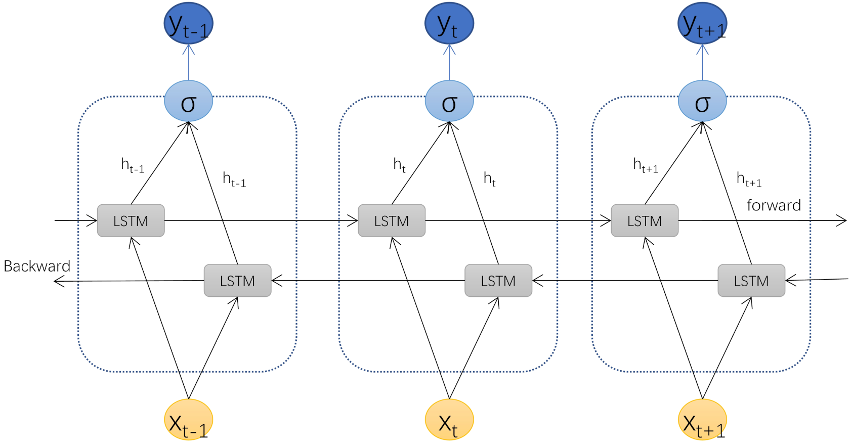
Generally, the LSTM network can only obtain information from the previous input, while the bidirectional long short-term memory (Bi-LSTM) model, as a cyclic neural network composed of two independent LSTM networks, can obtain information not only from the previous input but also from the future input state. The model design idea of Bi-LSTM is to make the characteristic data obtained at moment t have the information between the past and the future at the same time, and its principle structure is shown in Figure 3.
2.6. CNN-Bi-LSTM Model
The CNN-Bi-LSTM structure model proposed in this paper consists of one input layer, four convolution layers, two max pooling layers, four fully connected layers and one sigmoid output layer. At the same time, to prevent overfitting, a dropout layer is added between each fully connected layer to improve the generalization ability of the model. The data processed by the discrete wavelet transform are used as the input of the model, and the abstract features of the data are extracted by a convolutional neural network. Figure 4 shows the input of the bidirectional long short-term memory network (Bi-LSTM). These networks can cooperate with each other, retain the previous information, and further improve the ability to learn useful information from the EEG time-series data. After passing through the Bi-LSTM layer, the output features will be sent to three fully connected layers. Finally, the sigmoid output layer is added to the model for final recognition. The specific experimental steps are as follows. The shape of the input data (76 × 1) is obtained by discrete wavelet transform. Then, through the first convolutional layer, the abstract features of the input signal are extracted, and the number of one-dimensional convolution kernels in the Conv layer is 64. The shape of each convolution core is 3 × 1, and the stride of the convolution kernel is 1. After the convolutional layer is a rectified linear unit (ReLU) activation layer, which is added to the network to enhance the representation ability of the network and solve problems that cannot be solved by linear models. After the convolution and activation layers, the output will go through a max pooling layer to reduce dimensionality, remove redundant information, compress features, simplify network complexity, and reduce overfitting. The pooling window size is 2, and the step size is 2. Then, the higher-level features are further extracted through a three-layer convolution. The number of convolution kernels in Conv layer 1, Conv layer 2, and Conv layer 3 are 64, 128, and 128, respectively, all of which use the same 3 × 1 shape, and the activation function is the same as above. After layer 3, we add a max pooling layer. Finally, the resulting features are mapped to a fully connected layer with 256 neurons. Then, dropout is added to the fully connected layer. As shown in Figure 5, the fully connected layer plays the role of mapping the extracted distributed feature representation to the sample label space as the input of the Bi-LSTM network, and dropout can alleviate the overfitting problem to a certain extent. Both Bi-LSTM networks have 64 neurons. After the features are extracted by the Bi-LSTM network, the output signal is sent to three fully connected layers, and the hidden layers have 256, 128, and 64 neurons. Finally, the sigmoid output layer is added to the model for final recognition. To make the model output reach the optimal value, we use the Adam optimization algorithm to update and calculate the network parameters that affect the model training and output. The learning rate is 0.001, the number of epochs is 100, and the batch size is 200. An abstract illustration of the proposed approach is shown in Figure 6. First, the original signal is preprocessed, and then the discrete wavelet transform is used to decompose layer by layer to improve the signal-to-noise ratio. Next, a one-dimensional convolutional neural network and a bidirectional LSTM network are used to extract spatiotemporal features, and finally, classification is performed.
2.7. Model Performance Evaluation
In this study, four evaluation indicators are used to evaluate the performance of the architecture: accuracy, F1-score, precision and recall. These performance metrics are briefly described below:
Accuracy represents the ratio of the number of correct decisions to all the decisions.
Precision refers to the proportion of correctly predicted positive samples to all predicted positive samples.
Recall, also known as sensitivity or hit rate, refers to the proportion of positive samples that are correctly predicted.
The F1-score is an indicator of the comprehensive consideration of accuracy and recall rate.
3. Experimental Results and Analysis
To improve the generalization performance of the model and avoid the overfitting problem, dropout technology is introduced into the model, and the Adam optimizer is used to alleviate the gradient oscillation problem. The changes in training accuracy and training loss with the increase in epochs are shown in Figure 7. In this figure, the left vertical axis is the training accuracy, the right vertical axis is the training loss, the red curve is the training accuracy, and the blue curve is the training loss. Moreover, the accuracy and loss curves converge faster, the frustration is smaller, and the curves are smoother, which proves that our model has high robustness in this dataset.
Table 1 shows the comparison of our model with CNN and the LSTM and Bi-LSTM networks using performance indicators. From this table, we can see that the accuracy, precision, recall and F1-score achieved by our model are 99.32%, 99.01%, 98.87%, 98.93%, respectively, which are significantly better than those of the CNN [43], LSTM [44], Bi-LSTM [45], and CNN+Bi-LSTM models. Improvements of 2.37%, 7.71%, 11.08% and 2.03%, respectively, are observed when using this model. Among the CNN, LSTM, and Bi-LSTM models, CNN achieved the best classification accuracy of 96.95% because of its powerful feature extraction ability. Compared with the LSTM network, the Bi-LSTM network has the ability to consider the information from the front and back networks, so it has higher classification accuracy. We also compare the machine learning methods. As shown in Table 2, the classification accuracy of XGBoost [46] is 79.58%, the classification accuracy of graded CatBoost [47] is 94.14%, the classification accuracy of random forest (RF) [48] is 87.98%, and the classification accuracy of the support vector machine (SVM) [24] is 95.63%. The classification accuracy of the K-nearest neighbor (KNN) algorithm [27] is 94.23%. Our method is more robust than traditional machine learning methods.
Table 3 shows a comparison of our proposed DWT-CNN-Bi-LSTM architecture with existing technologies. Most of the existing models are based on machine learning. These machine learning models use handmade features, which require domain knowledge and are difficult to apply. Farsi et al. proposed a deep learning method based on an LSTM network to automatically extract time-series information from EEG data. However, there is no suitable mechanism for dealing with spatial information. Our proposed CNN-Bi-LSTM model can automatically extract hidden spatiotemporal information from EEG signals, which has more advantages than some existing machine learning and deep learning methods.
4. Conclusions and Prospects
In this paper, a deep learning framework integrated with the DWT, CNN and Bi-LSTM network is proposed and used to automatically extract and classify the time-series features of alcohol EEG signals. In this method, the data are preprocessed through standard deviation standardization and discrete wavelet transform, and then the denoised data are input into the CNN-Bi-LSTM network. The average classification accuracy of this method is 99.32%, the accuracy is 99.01%, and the recall rate is 98.87%. This mechanism is superior to the existing multichannel EEG signals in predicting alcoholism and has high accuracy and reliability. The experimental results show that automatic feature extraction from EEG signals by deep learning has more advantages than manual feature extraction. In recent years, with the development of the Internet of Things and the improvement of people’s economic level, an increasing number of people have begun to pay attention to their own health problems. Medical wearable devices can upload the wearer’s body information in real-time and respond in time to ensure the health of patients. The deep learning strategy proposed by the study can provide a new and powerful diagnostic scheme for medical wearable devices. Similarly, our proposed deep learning model can also be extended to epilepsy diagnosis, emotion recognition and other applications through EEG classification. It is also an effective deep learning model for signals such as ECG and EMG.
Author Contributions
Conceptualization, L.W. and H.L.; methodology, H.L.; software, H.L.; validation, H.L., L.W.; formal analysis, H.L.; investigation, H.L.; data curation, H.L.; writing—original draft preparation, H.L.; writing—review and editing, L.W.; supervision, L.W.; project administration, L.W. All authors have read and agreed to the published version of the manuscript.
Funding
This research received no external funding.
Institutional Review Board Statement
Not applicable.
Informed Consent Statement
Not applicable.
Data Availability Statement
All data related to the research are presented in the article.
Conflicts of Interest
The authors declare no conflict of interest.
References
- World Health Organization. Global Status Report on Alcohol and Health 2018; World Health Organization: Geneva, Switzerland, 2019; Available online: https://www.who.int/publications/i/item/9789241565639 (accessed on 25 April 2022).
- Rocco, A.; Compare, D.; Angrisani, D.; Zamparelli, M.S.; Nardone, G. Alcoholic disease: Liver and beyond. World J. Gastroenterol. WJG 2014, 20, 14652. [Google Scholar] [CrossRef] [PubMed]
- Harper, C. The neurotoxicity of alcohol. Hum. Exp. Toxicol. 2007, 26, 251–257. [Google Scholar] [CrossRef] [PubMed]
- Brust, J. Ethanol and cognition: Indirect effects, neurotoxicity and neuroprotection: A review. Int. J. Environ. Res. Public Health 2010, 7, 1540–1557. [Google Scholar] [CrossRef] [PubMed]
- Han, D.X.; Zhou, C.D.; Liu, Y.H. The neurotoxicity of alcohol. Appl. Brain State Relat. EEG Complex. Meas. Ment. Workload Eval. 2001, 14, 102–106. [Google Scholar]
- Noachtar, S.; Rémi, J. The role of EEG in epilepsy: A critical review. Epilepsy Behav. 2009, 15, 22–33. [Google Scholar] [CrossRef]
- Taran, S.; Bajaj, V. Rhythm-based identification of alcohol EEG signals in IET science Meas. IET Sci. Meas. Technol. 2018, 12, 343–349. [Google Scholar] [CrossRef]
- Mumtaz, W.; Vuong, P.L.; Malik, A.S.; Rashid, R.B.A. A review on EEG-based methods for screening and diagnosing alcohol use disorder. Cogn. Neurodynamics 2018, 12, 141–156. [Google Scholar] [CrossRef]
- Bavkar, S.; Iyer, B.; Deosarkar, S. Rapid screening of alcoholism: An EEG based optimal channel selection approach. IEEE Access 2019, 7, 99670–99682. [Google Scholar] [CrossRef]
- Pollock, V.E.; Volavka, J.; Goodwin, D.W.; Mednick, S.A.; Gabrielli, W.F.; Knop, J.; Schulsinger, F. The EEG after alcohol administration in men at risk for alcoholism. Arch. Gen. Psychiatry 1983, 40, 857–861. [Google Scholar] [CrossRef]
- Acharya, U.R.; Sree, S.V.; Chattopadhyay, S.; Yu, W.; Ang, P.C.A. Application of recurrence quantification analysis for the automated identification of epileptic EEG signals. Int. J. Neural Syst. 2011, 21, 199–211. [Google Scholar] [CrossRef]
- Ball, T.; Kern, M.; Mutschler, I.; Aertsen, A.; Schulze-Bonhage, A. Signal quality of simultaneously recorded invasive and non-invasive EEG. Neuroimage 2009, 46, 708–716. [Google Scholar] [CrossRef] [PubMed] [Green Version]
- Crespo-Garcia, M.; Atienza, M.; Cantero, J.L. Muscle artifact removal from human sleep EEG by using independent component analysis. Ann. Biomed. Eng. 2008, 36, 467–475. [Google Scholar] [CrossRef] [PubMed]
- Pradhan, N.; Sadasivan, P.K.; Arunodaya, G.R. Detection of seizure activity in EEG by an artificial neural network: A preliminary study. Comput. Biomed. Res. 1996, 29, 303–313. [Google Scholar] [CrossRef] [PubMed]
- Acharya, U.R.; Molinari, F.; Sree, S.V.; Chattopadhyay, S.; Ng, K.H.; Suri, J.S. Automated diagnosis of epileptic EEG using entropies. Biomed. Signal Process. Control 2012, 7, 401–408. [Google Scholar] [CrossRef] [Green Version]
- Übeyli, E.D. Least squares support vector machine employing model-based methods coefficients for analysis of EEG signals. Expert Syst. Appl. 2010, 37, 233–239. [Google Scholar] [CrossRef]
- Akin, M. Comparison of wavelet transform and FFT methods in the analysis of EEG signals. J. Med. Syst. 2002, 26, 241–247. [Google Scholar] [CrossRef]
- Petrantonakis, P.C.; Hadjileontiadis, L.J. Adaptive emotional information retrieval from EEG signals in the time-frequency domain. IEEE Trans. Signal Process. 2012, 60, 2604–2616. [Google Scholar] [CrossRef]
- Subasi, A.; Gursoy, M.I. EEG signal classification using PCA, ICA, LDA and support vector machines. Expert Syst. Appl. 2010, 37, 8659–8666. [Google Scholar] [CrossRef]
- Li, S.; Zhou, W.; Yuan, Q.; Geng, S.; Cai, D. Feature extraction and recognition of ictal EEG using EMD and SVM. Comput. Biol. Med. 2013, 43, 807–816. [Google Scholar] [CrossRef]
- Bavkar, S.; Iyer, B.; Deosarkar, S. The role of EEG in epilepsy: A critical review. Biocybern. Biomed. Eng. 2021, 41, 83–96. [Google Scholar] [CrossRef]
- Al-Qazzaz, N.K.; Hamid, B.; Mohd, A.S.; Ahmad, S.A.; Islam, M.S.; Escudero, J. Automatic artifact removal in EEG of normal and demented individuals using ICA–WT during working memory tasks. Sensors 2017, 17, 1326. [Google Scholar] [CrossRef] [PubMed]
- Kıymık, M.K.; Güler, İ.; Dizibüyük, A.; Akın, M. Comparison of STFT and wavelet transform methods in determining epileptic seizure activity in EEG signals for real-time application. Comput. Biol. Med. 2005, 35, 603–6166. [Google Scholar] [CrossRef] [PubMed]
- Acharya, U.R.; Sree, S.V.; Chattopadhyay, S.; Suri, J.S. Automated diagnosis of normal and alcoholic EEG signals. Int. J. Neural Syst. 2012, 22, 1250011. [Google Scholar] [CrossRef] [PubMed]
- Faust, O.; Acharya, R.U.; Allen, A.R.; Lin, C.M. Analysis of EEG signals during epileptic and alcoholic states using AR modeling techniques. Irbm 2008, 29, 44–52. [Google Scholar] [CrossRef]
- Bajaj, V.; Guo, Y.; Sengur, A.; Siuly, S.; Alcin, O.F. A hybrid method based on time–frequency images for classification of alcohol and control EEG signals. Neural Comput. Appl. 2017, 28, 3717–3723. [Google Scholar] [CrossRef] [Green Version]
- Faust, O.; Yu, W.; Kadri, N.A. Computer-based identification of normal and alcoholic EEG signals using wavelet packets and energy measures. J. Mech. Med. Biol. 2013, 13, 1350033. [Google Scholar] [CrossRef]
- Sharma, M.; Sharma, P.; Pachori, R.B.; Acharya, U.R. Dual-tree complex wavelet transform-based features for automated alcoholism identification. Int. J. Fuzzy Syst. 2018, 4, 1297–1308. [Google Scholar] [CrossRef]
- Wang, H.; Zhang, Y. An efficient framework for the analysis of big brain signals data. In Australasian DATABASE Conference; Springer: Cham, Switzerland, 2018; pp. 199–207. [Google Scholar]
- Salankar, N.; Qaisar, S.M.; Pławiak, P.; Tadeusiewicz, R.; Hammad, M. EEG based alcoholism detection by oscillatory modes decomposition second order difference plots and machine learning. Biocybern. Biomed. Eng. 2022, 42, 173–186. [Google Scholar] [CrossRef]
- Patidar, S.; Pachori, R.B.; Upadhyay, A.; Acharya, U.R. An integrated alcoholic index using tunable-Q wavelet transform based features extracted from EEG signals for diagnosis of alcoholism. Appl. Soft Comput. 2017, 50, 71–78. [Google Scholar] [CrossRef]
- Rodrigues, J.D.C.; Filho Rebouças, P.P.; Peixoto, E., Jr.; Kumar, A.; de Albuquerque, V.H.C. Classification of EEG signals to detect alcoholism using machine learning techniques. Pattern Recognit. Lett. 2019, 125, 140–149. [Google Scholar] [CrossRef]
- Flathau, D.; Breitenbach, J.; Baumgartl, H.; Buettner, R. Early Detection of Alcohol Use Disorder Based on a Novel Machine Learning Approach Using EEG Data. In Proceedings of the 2021 IEEE International Conference on Big Data (Big Data), Orlando, FL, USA, 15–18 December 2021; pp. 3897–3904. [Google Scholar]
- Farsi, L.; Siuly, S.; Kabir, E.; Wang, H. Classification of alcoholic EEG signals using a deep learning method. IEEE Sens. J. 2020, 21, 3552–3560. [Google Scholar] [CrossRef]
- Ildar, R. Deep learning and machine learning for EEG signal processing on the example of recognizing the disease of alcoholism. medRxiv 2021. [Google Scholar] [CrossRef]
- Mukhtar, H.; Qaisar, S.M.; Zaguia, A. Deep convolutional neural network regularization for alcoholism detection using EEG signals. Sensors 2021, 21, 5456. [Google Scholar] [CrossRef] [PubMed]
- Kumari, N.; Anwar, S.; Bhattacharjee, V. A Deep Learning-Based Approach for Accurate Diagnosis of Alcohol Usage Severity Using EEG Signals. IETE J. Res. 2022, 1–15. [Google Scholar] [CrossRef]
- Begleiter, H. EEG Database Machine Learning Repository. Available online: http://archive.ics.uci.edu/ml/datasets/EEG%20Database (accessed on 13 April 2022).
- Thara, D.K.; PremaSudha, B.G.; Xiong, F. Auto-detection of epileptic seizure events using deep neural network with different feature scaling techniques. Pattern Recognit. Lett. 2019, 128, 544–550. [Google Scholar]
- Kumar, Y.; Dewal, M.L.; Anand, R.S. Epileptic seizure detection using DWT based fuzzy approximate entropy and support vector machine. Neurocomputing 2014, 133, 271–279. [Google Scholar] [CrossRef]
- Radenović, F.; Tolias, G.; Chum, O. Fine-tuning CNN image retrieval with no human annotation. IEEE Trans. Pattern Anal. Mach. Intell. 2018, 41, 1655–1668. [Google Scholar] [CrossRef] [Green Version]
- Xu, G.; Ren, T.; Chen, Y.; Che, W. A one-dimensional cnn-lstm model for epileptic seizure recognition using eeg signal analysis. Front. Neurosci. 2020, 14, 1253. [Google Scholar] [CrossRef]
- O’Shea, K.; Nash, R. An introduction to convolutional neural networks. arXiv 2015, arXiv:1511.08458. [Google Scholar]
- Hochreiter, S.; Schmidhuber, J. Long short-term memory. Neural Comput. 1997, 9, 1735–1780. [Google Scholar] [CrossRef]
- Yang, J.; Huang, X.; Wu, H.; Yang, X. EEG-based emotion classification based on bidirectional long short-term memory network. Procedia Comput. Sci. 2020, 174, 491–504. [Google Scholar] [CrossRef]
- Parui, S.; Bajiya, A.K.R.; Samanta, D.; Chakravorty, N. Emotion recognition from EEG signal using XGBoost algorithm. In Proceedings of the 2019 IEEE 16th India Council International Conference (INDICON), Rajkot, India, 13–15 December 2019; pp. 1–4. [Google Scholar]
- Lee, S.B.; Kim, Y.J.; Hwang, S.; Son, H.; Lee, S.K.; Park, K.I.; Kim, Y.G. Predicting Parkinson’s disease using gradient boosting decision tree models with electroencephalography signals. Park. Relat. Disord. 2022, 95, 77–85. [Google Scholar] [CrossRef] [PubMed]
- Fraiwan, L.; Lweesy, K.; Khasawneh, N.; Wenz, H.; Dickhaus, H. Automated sleep stage identification system based on time–frequency analysis of a single EEG channel and random forest classifier. Comput. Methods Programs Biomed. 2012, 108, 10–19. [Google Scholar] [CrossRef] [PubMed]
- Sharma, M.; Deb, D.; Acharya, U.R. A novel three-band orthogonal wavelet filter bank method for an automated identification of alcoholic EEG signals. Appl. Intell. 2018, 48, 1368–1378. [Google Scholar] [CrossRef]
- Bavkar, S.; Iyer, B.; Deosarkar, S. Detection of alcoholism: An EEG hybrid features and ensemble subspace K-NN based approach. Int. Conf. Distrib. Comput. Internet Technol. 2019, 11319, 161–168. [Google Scholar]
Figure 1.
Sample (a) and sample (b) are alcoholic and normal EEG signals, respectively.

Figure 2.
LSTM network structure.

Figure 3.
BI-LSTM network structure.

Figure 4.
CNN network structure.

Figure 5.
CNN network structure.

Figure 6.
CNN network structure.

Figure 7.
Training accuracy and training loss.


Table 1.
Performance of different deep learning models in binary classification tasks.
| Methods | Accuracy | Precision | Recall | F1-Score |
|---|---|---|---|---|
| CNN | 96.95% | 96.05% | 95.70% | 96.58% |
| Bi-LSTM | 91.61% | 91.60% | 90.41% | 91.39% |
| LSTM | 88.24% | 88.42% | 87.98% | 89.21% |
| CNN+Bi-LSTM | 97.29% | 96.89% | 97.13% | 96.93% |
| Our model | 99.32% | 99.01% | 98.87% | 98.93% |
Table 2.
Mainstream classification methods and comparison of our proposed models.
| Comparison of Different Models | ||||||
|---|---|---|---|---|---|---|
| Model | XGBoost | CatBoost | RF | SVM | KNN | Our Model |
| Accuracy | 79.58% | 94.14% | 87.98% | 95.63% | 94.23% | 99.32% |
Table 3.
Comparison of DWT-CNN-Bi-LSTM architecture with existing methods.
| Reference | Feature Extraction | Classifier | Accuracy |
|---|---|---|---|
| Acharya et al. [24] | Approximate Entrop LLE Sample Entropy Higher Order Spectra | SVM | 91.7% |
| Faust et al. [27] | Wavelet Packet Decomposition | K-NN | 95.8% |
| Patidar et al. [31] | Tunable-Q Wavelet Transform Centered Correntropy PCA | LS-SVM | 97.02% |
| Farsi et al. [34] | Improved Binary Principal Component Analysis | ANN LSTM | 93% |
| Sharma et al. [49] | Three-band Orthogonal Wavelet Filter Bank | LS-SVM | 97.08% |
| Ildar et al. [35] | Wavelet transforms | CNN | 86% |
| Bavkar et al. [50] | Linear Nonlinear Statistical Feature | K-NN | 98.25% |
| Mukhtar H et al. [36] | CNN | CNN with 3 convolution layers, dropout | 98.00% |
| N Kumari et al. [37] | None | CNN LSTM CNN + LSTM | 92.77% 89% 91% |
| Our model | Discrete Wavelet Transformation | CNN Bi-LSTM | 99.32% |
Publisher’s Note: MDPI stays neutral with regard to jurisdictional claims in published maps and institutional affiliations. |
© 2022 by the authors. Licensee MDPI, Basel, Switzerland. This article is an open access article distributed under the terms and conditions of the Creative Commons Attribution (CC BY) license (https://creativecommons.org/licenses/by/4.0/).
Share and Cite
MDPI and ACS Style
Li, H.; Wu, L. EEG Classification of Normal and Alcoholic by Deep Learning. Brain Sci. 2022, 12, 778. https://doi.org/10.3390/brainsci12060778
AMA Style
Li H, Wu L. EEG Classification of Normal and Alcoholic by Deep Learning. Brain Sciences. 2022; 12(6):778. https://doi.org/10.3390/brainsci12060778
Chicago/Turabian StyleLi, Houchi, and Lei Wu. 2022. "EEG Classification of Normal and Alcoholic by Deep Learning" Brain Sciences 12, no. 6: 778. https://doi.org/10.3390/brainsci12060778
Note that from the first issue of 2016, this journal uses article numbers instead of page numbers. See further details here.