Multi Objective for PMU Placement in Compressed Distribution Network Considering Cost and Accuracy of State Estimation


Abstract
:1. Introduction
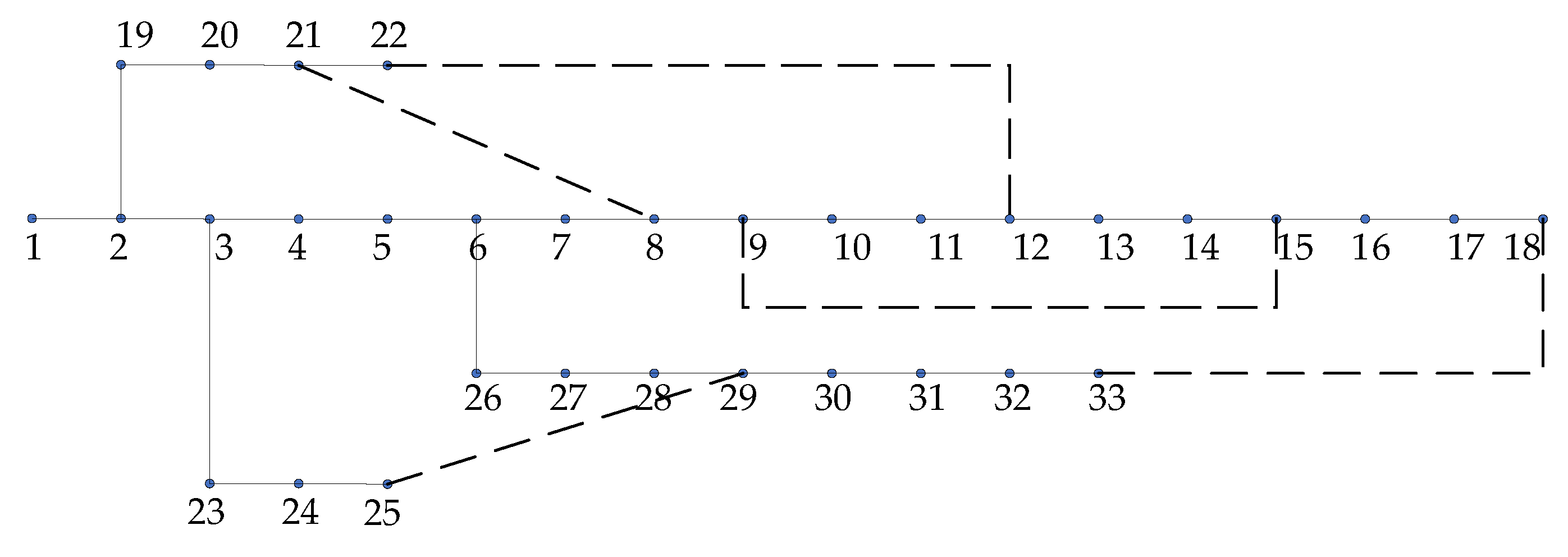
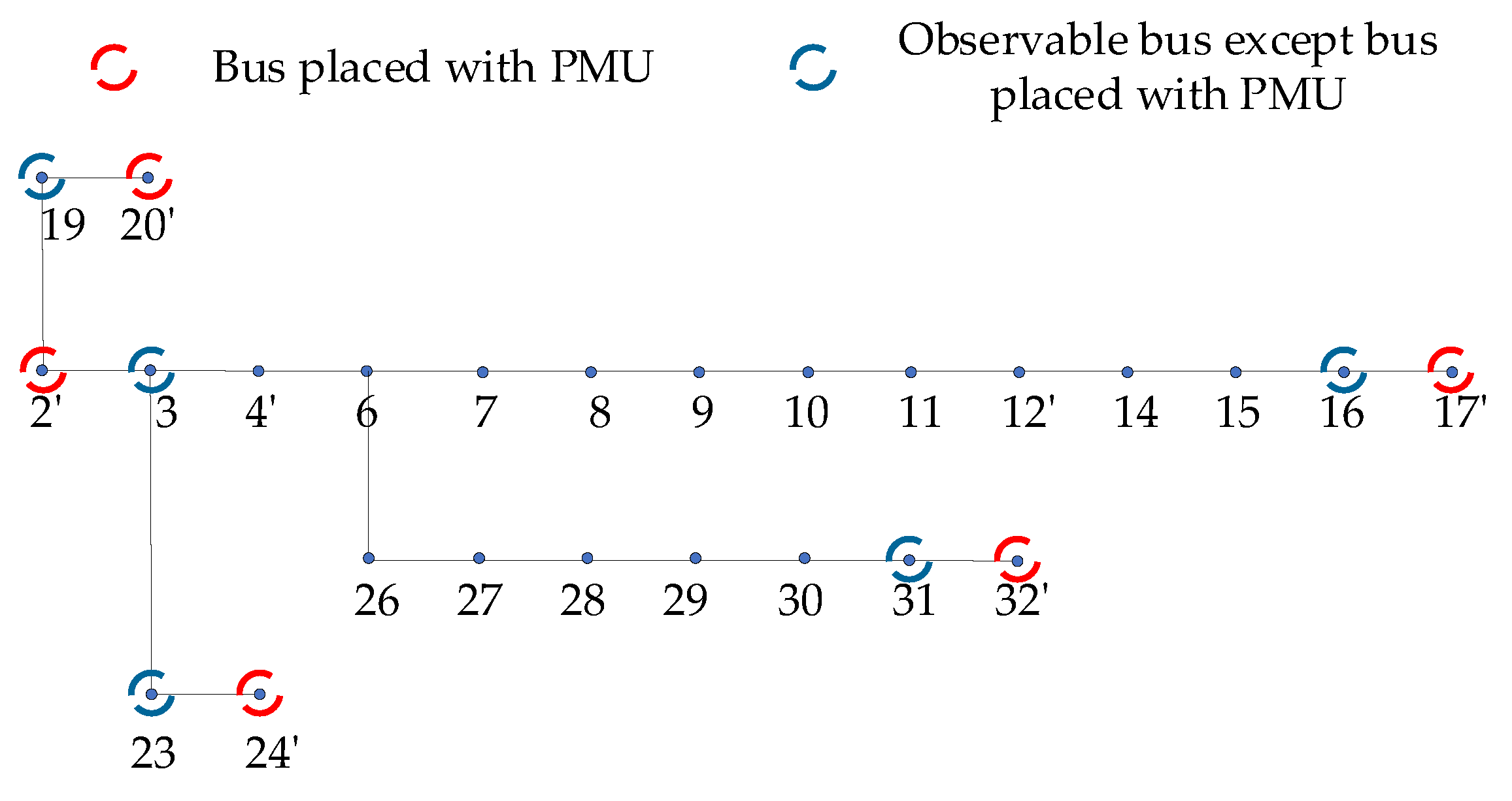
2. Network Compression
2.1. The Observability of Distribution Network
2.2. Network Compression Based on Pre-Configuration and Existing Measurements
3. Hybrid State Estimator Considering PMU Measurements
3.1. The Basic Model of State Estimation
3.2. Estimator with PMU Measurements
4. Multi Objective Model of Optimal PMU Placement
4.1. The Basic Model of OPP Considering Cost and State Estimation Accuracy
4.2. Updated Constraint Considering ZIB Measurement
4.3. Updated Constraint Considering SCADA Measurement
4.4. The Final OPP Model
5. Solution Methodology Based on NSGA-II and TOPSIS
5.1. Optimization Based on NSGA-II
5.1.1. Initialization Based on Network Compression
5.1.2. Fitness Calculation
5.1.3. Genetic Operations Based on Pre-Configuration
5.1.4. Fast Nondominated Sorting
5.1.5. Crowding-Distance Calculation
5.1.6. Optimization Process
5.2. Selection Based on TOPSIS
6. Simulation Results and Discussion
7. Conclusions
Author Contributions
Funding
Conflicts of Interest
Appendix A


References
- Hassan, E.; Napis, N.; Khatib, T.; Abd Kadir, A.; Sulaima, M. An improved method for reconfiguring and optimizing electrical active distribution network using evolutionary particle swarm optimization. Appl. Sci. 2018, 8, 804. [Google Scholar] [CrossRef]
- Al Essa, M.; Cipcigan, L. Reallocating charging loads of electric vehicles in distribution networks. Appl. Sci. 2016, 6, 53. [Google Scholar] [CrossRef]
- Cui, K.; Yong, C.; E, Z.; Kong, X.; Chen, Y.; Wang, X. Multiobjective scheduling of an active distribution network based on coordinated optimization of source network load. Appl. Sci. 2018, 8, 1888. [Google Scholar] [CrossRef]
- Tan, Y.; Liu, W.; Su, J.; Bai, X. Generative adversarial networks based heterogeneous data integration and its application for intelligent power distribution and utilization. Appl. Sci. 2018, 8, 93. [Google Scholar] [CrossRef]
- Prasad, S.; Kumar, D.M.V. Trade-offs in PMU and IED deployment for active distribution state estimation using multi-objective evolutionary algorithm. IEEE Trans. Instrum. Meas. 2018, 67, 1298–1307. [Google Scholar] [CrossRef]
- Mabaning, A.A.G.; Orillaza, J.R.C.; Von Meier, A. Optimal PMU placement for distribution networks. In Proceedings of the 2017 IEEE Innovative Smart Grid Technologies-Asia (ISGT-Asia), Auckland, New Zealand, 4–7 December 2017; pp. 1–6. [Google Scholar] [CrossRef]
- Jamei, M.; Scaglione, A.; Roberts, C.; Stewart, E.; Peisert, S.; McParland, C.; McEachern, A. Anomaly detection using optimally placed μPMU sensors in distribution grids. IEEE Trans. Power Syst. 2017, 33, 3611–3623. [Google Scholar] [CrossRef]
- Hooshyar, H.; Baran, M.E.; Firouzi, S.R.; Vanfretti, L. PMU-assisted overcurrent protection for distribution feeders employing Solid State Transformers. Sustain. Energy Grids Netw. 2017, 10, 26–34. [Google Scholar] [CrossRef]
- Mahmood, F.; Hooshyar, H.; Lavenius, J.; Bidadfar, A.; Lund, P.; Vanfretti, L. Real-time reduced steady-state model synthesis of active distribution networks using PMU measurements. IEEE Trans. Power Deliv. 2017, 32, 546–555. [Google Scholar] [CrossRef]
- Cavraro, G.; Arghandeh, R. Power distribution network topology detection with time-series signature verification method. IEEE Trans. Power Syst. 2018, 33, 3500–3509. [Google Scholar] [CrossRef]
- Shahsavari, A.; Sadeghi-Mobarakeh, A.; Stewart, E.M.; Cortez, E.; Alvarez, L.; Megala, F.; Mohsenian-Rad, H. Distribution grid reliability versus regulation market efficiency: An analysis based on micro-PMU data. IEEE Trans. Smart Grid 2017, 8, 2916–2925. [Google Scholar] [CrossRef]
- Mahaei, S.M.; Hagh, M.T. Minimizing the number of PMUs and their optimal placement in power systems. Electr. Power Syst. Res. 2012, 83, 66–72. [Google Scholar] [CrossRef]
- Korres, G.N.; Georgilakis, P.S.; Koutsoukis, N.C.; Manousakis, N.M. Numerical observability method for optimal phasor measurement units placement using recursive Tabu search method. IET Gener. Transm. Distrib. 2013, 7, 347–356. [Google Scholar] [CrossRef]
- Khorram, E.; Taleshian Jelodar, M. PMU placement considering various arrangements of lines connections at complex buses. Int. J. Electr. Power Energy Syst. 2018, 94, 97–103. [Google Scholar] [CrossRef]
- Rahman, N.H.A.; Zobaa, A.F. Integrated mutation strategy with modified binary PSO algorithm for optimal PMUs placement. IEEE Trans. Ind. Inform. 2017, 13, 3124–3133. [Google Scholar] [CrossRef]
- Aghaei, J.; Baharvandi, A.; Rabiee, A.; Akbari, M.A. Probabilistic PMU placement in electric power networks: An MILP-based multiobjective model. IEEE Trans. Ind. Inform. 2015, 11, 332–341. [Google Scholar] [CrossRef]
- Nikkhah, S.; Aghaei, J.; Safarinejadian, B.; Norouzi, M.-A. Contingency constrained phasor measurement units placement with n − k redundancy criterion: A robust optimisation approach. IET Sci. Meas. Technol. 2017, 12, 151–160. [Google Scholar] [CrossRef]
- Asgari, A.; Firouzjah, K.G. Optimal PMU placement for power system observability considering network expansion and N−1 contingencies. IET Gener. Transm. Distrib. 2018, 12, 4216–4224. [Google Scholar] [CrossRef]
- Alimardani, A.; Therrien, F.; Atanackovic, D.; Jatskevich, J.; Vaahedi, E. Distribution system state estimation based on nonsynchronized smart meters. IEEE Trans. Smart Grid 2015, 6, 2919–2928. [Google Scholar] [CrossRef]
- Primadianto, A.; Lu, C.N. A review on distribution system state estimation. IEEE Trans. Power Syst. 2017, 32, 3875–3883. [Google Scholar] [CrossRef]
- Suh, J.; Hwang, S.; Jang, G. Development of a transmission and distribution integrated monitoring and analysis system for high distributed generation penetration. Energies 2017, 10, 1282. [Google Scholar] [CrossRef]
- Pau, M.; Ponci, F.; Monti, A.; Angioni, A.; Muscas, C.; Pegoraro, P.A.; Sulis, S. Bayesian approach for distribution system state estimation with non-gaussian uncertainty models. IEEE Trans. Instrum. Meas. 2017, 66, 2957–2966. [Google Scholar] [CrossRef]
- Angioni, A.; Schlösser, T.; Ponci, F.; Monti, A. Impact of pseudo-measurements from new power profiles on state estimation in low-voltage grids. IEEE Trans. Instrum. Meas. 2016, 65, 70–77. [Google Scholar] [CrossRef]
- Ou, T.C.; Lu, K.H.; Huang, C.J. Improvement of transient stability in a hybrid power multi-system using a designed NIDC (Novel Intelligent Damping Controller). Energies 2017, 10, 488. [Google Scholar] [CrossRef]
- Su, H.Y.; Liu, T.Y. A PMU-based method for smart transmission grid voltage security visualization and monitoring. Energies 2017, 10, 1103. [Google Scholar] [CrossRef]
- Usman, M.U.; Faruque, M.O. Validation of a PMU-based fault location identification method for smart distribution network with photovoltaics using real-time data. IET Gener. Transm. Distrib. 2018, 12, 5824–5833. [Google Scholar] [CrossRef]
- Ou, T.C.; Hong, C.M. Dynamic operation and control of microgrid hybrid power systems. Energy 2014, 66, 314–323. [Google Scholar] [CrossRef]
- Muscas, C.; Pau, M.; Pegoraro, P.A.; Sulis, S. Effects of measurements and pseudomeasurements correlation in distribution system state estimation. IEEE Trans. Instrum. Meas. 2014, 63, 2813–2823. [Google Scholar] [CrossRef]
- Dzafic, I.; Jabr, R.A.; Huseinagic, I.; Pal, B.C. Multi-phase state estimation featuring industrial-grade distribution network models. IEEE Trans. Smart Grid 2017, 8, 609–618. [Google Scholar] [CrossRef]
- Pau, M.; Pegoraro, P.A.; Sulis, S. Efficient branch-current-based distribution system state estimation including synchronized measurements. IEEE Trans. Instrum. Meas. 2013, 62, 2419–2429. [Google Scholar] [CrossRef]
- Mouwafi, M.T.; El-Sehiemy, R.A.; Abou El-Ela, A.A.; Kinawy, A.M. Optimal placement of phasor measurement units with minimum availability of measuring channels in smart power systems. Electr. Power Syst. Res. 2016, 141, 421–431. [Google Scholar] [CrossRef]
- Rahman, N.H.A.; Zobaa, A.F. Optimal PMU placement using topology transformation method in power systems. J. Adv. Res. 2016, 7, 625–634. [Google Scholar] [CrossRef]
- Esmaili, M. Inclusive multi-objective PMU placement in power systems considering conventional measurements and contingencies. Int. Trans. Electr. Energy Syst. 2016, 26, 609–626. [Google Scholar] [CrossRef]
- Khajeh, K.G.; Bashar, E.; Rad, A.M.; Gharehpetian, G.B. Integrated model considering effects of zero injection buses and conventional measurements on optimal PMU placement. IEEE Trans. Smart Grid 2017, 8, 1006–1013. [Google Scholar] [CrossRef]
- Jamil, E.; Rihan, M.; Anees, M.A. Towards optimal placement of phasor measurement units for smart distribution systems. In Proceedings of the 2014 6th IEEE Power India International Conference (PIICON), Delhi, India, 5–7 December 2014; pp. 1–6. [Google Scholar] [CrossRef]
- Manousakis, N.M.; Korres, G.N. A weighted least squares algorithm for optimal PMU placement. IEEE Trans. Power Syst. 2013, 28, 3499–3500. [Google Scholar] [CrossRef]
- Aminifar, F.; Fotuhi-Firuzabad, M.; Safdarian, A. Optimal PMU placement based on probabilistic cost/benefit analysis. IEEE Trans. Power Syst. 2013, 28, 566–567. [Google Scholar] [CrossRef]
- Li, Q.; Cui, T.; Weng, Y.; Negi, R.; Franchetti, F.; Ilic, M.D. An information-theoretic approach to PMU placement in electric power systems. IEEE Trans. Smart Grid 2013, 4, 446–456. [Google Scholar] [CrossRef]
- Maji, T.K.; Acharjee, P. Multiple solutions of optimal PMU placement using exponential binary PSO algorithm for smart grid applications. IEEE Trans. Ind. Appl. 2017, 53, 2550–2559. [Google Scholar] [CrossRef]
- Jamuna, K.; Swarup, K.S. Multi-objective biogeography based optimization for optimal PMU placement. Appl. Soft Comput. J. 2012, 12, 1503–1510. [Google Scholar] [CrossRef]
- Shafiullah, M.; Abido, M.A.; Ismail Hossain, M.; Mantawy, A.H. An improved OPP problem formulation for distribution grid observability. Energies 2018, 11, 3069. [Google Scholar] [CrossRef]
- Gopakumar, P.; Jaya Bharata Reddy, M.; Mohanta, D.K. Pragmatic multi-stage simulated annealing for optimal placement of synchrophasor measurement units in smart power grids. Front. Energy 2015, 9, 148–161. [Google Scholar] [CrossRef]
- Kazemi Karegar, H.; Dalali, M. Optimal PMU placement for full observability of the power network with maximum redundancy using modified binary cuckoo optimisation algorithm. IET Gener. Transm. Distrib. 2016, 10, 2817–2824. [Google Scholar] [CrossRef]
- Khiabani, V.; Erdem, E.; Farahmand, K.; Nygard, K. Genetic algorithm for instrument placement in smart grid. In Proceedings of the 2013 World Congress on Nature and Biologically Inspired Computing, Fargo, ND, USA, 12–14 August 2013; pp. 214–219. [Google Scholar] [CrossRef]
- Shi, L.; Yang, S.L.; Li, K.; Yu, B. Developing an evaluation approach for software trustworthiness using combination weights and TOPSIS. J. Softw. 2012, 7, 532–543. [Google Scholar] [CrossRef]
- Zhou, X.; Sun, H.; Zhang, C.; Dai, Q. Optimal placement of PMUs using adaptive genetic algorithm considering measurement redundancy. Int. J. Reliab. Qual. Saf. Eng. 2016, 23, 1640001. [Google Scholar] [CrossRef]
- Abdelsalam, H.A.; Abdelaziz, A.Y.; Osama, R.A.; Salem, R.H. Impact of distribution system reconfiguration on optimal placement of phasor measurement units. In Proceedings of the 2014 Clemson University Power Systems Conference, Clemson, SC, USA, 11–14 March 2014; pp. 1–6. [Google Scholar] [CrossRef]
- Chen, X.; Chen, T.; Tseng, K.J.; Sun, Y.; Amaratunga, G. Customized optimal μPMU placement method for distribution networks. In Proceedings of the 2016 IEEE PES Asia-Pacific Power and Energy Engineering Conference (APPEEC), Xi’an, China, 25–28 October 2016; pp. 135–140. [Google Scholar] [CrossRef]


| Case | Optimal Solution | No. of PMUs | State Estimation Error |
|---|---|---|---|
| 1: Without Network Compression | The Most Economical Solution | 11 | 6.64328588 × 10^(–4) |
| The Compromised Solution | 12 | 6.46038299 × 10^(–4) | |
| 2: With Network Compression | The Most Economical Solution | 10 | 6.38764872 × 10^(–4) |
| The Compromised Solution | 11 | 6.13058913 × 10^(–4) |
| Method | IEEE 33 Bus System | IEEE 34 Bus System | IEEE 69 Bus System | |||
|---|---|---|---|---|---|---|
| No. of PMUs | PMU Locations | No. of PMUs | PMU Locations | No. of PMUs | PMU Locations | |
| Proposed Method (The Most Economical Solution) | 10 | 2, 8, 11, 15, 17, 20, 24, 26, 30, 32 | 11 | 2, 4, 6, 10, 12, 17, 21, 23, 28, 31, 33 | 22 | 2, 3, 8, 11, 14, 17, 22, 26, 28, 33, 34, 37, 41, 45, 49, 51, 56, 59, 62, 64, 66, 68 |
| Proposed Method (The Compromised Solution) | 11 | 2, 4, 8, 11, 15, 17, 20, 24, 26, 30, 32 | 12 | 2, 4, 6, 10, 12, 17, 20, 21, 23, 28, 31, 33 | 23 | 2, 3, 8, 11, 12, 14, 17, 22, 26, 28, 33, 34, 37, 41, 45, 49, 51, 56, 59, 62, 64, 66, 68 |
| Reference [46] | 11 | 2, 6, 8, 11, 15, 17, 21, 24, 28, 29, 32 | 12 | 2, 5, 7, 10, 13, 17, 21, 24, 28, 30, 31, 33 | 26 | 1, 4, 8, 14, 17, 19, 21, 24, 27, 28, 31, 34, 37, 39, 42, 45, 49, 51, 54, 56, 59, 61, 64, 66, 68, 69 |
| Reference [47] | 14 | 2, 4, 6, 8, 11, 13, 15, 17, 21, 23, 24, 27, 29, 32 | 13 | 2, 4, 8, 12, 14, 16, 17, 21, 24, 27, 28, 31, 33 | 27 | 1, 4, 5, 8, 9, 12, 15, 18, 20, 23, 26, 29, 32, 34, 37, 40, 42, 45, 49, 52, 53, 55, 58, 61, 64, 66, 69 |
| Reference [48] | 11 | 2, 5, 8, 11, 14, 17, 21, 24, 27, 30, 32 | 13 | 2, 4, 8, 10, 12, 17, 21, 23, 25, 28, 31, 33 | 25 | 2, 4, 7, 9, 14, 17, 20, 23, 26, 29, 32, 34, 37, 40, 43, 45, 49, 51, 54, 57, 58, 61, 64, 66, 68 |
© 2019 by the authors. Licensee MDPI, Basel, Switzerland. This article is an open access article distributed under the terms and conditions of the Creative Commons Attribution (CC BY) license (http://creativecommons.org/licenses/by/4.0/).
Share and Cite
Kong, X.; Wang, Y.; Yuan, X.; Yu, L. Multi Objective for PMU Placement in Compressed Distribution Network Considering Cost and Accuracy of State Estimation. Appl. Sci. 2019, 9, 1515. https://doi.org/10.3390/app9071515
Kong X, Wang Y, Yuan X, Yu L. Multi Objective for PMU Placement in Compressed Distribution Network Considering Cost and Accuracy of State Estimation. Applied Sciences. 2019; 9(7):1515. https://doi.org/10.3390/app9071515
Chicago/Turabian StyleKong, Xiangyu, Yuting Wang, Xiaoxiao Yuan, and Li Yu. 2019. "Multi Objective for PMU Placement in Compressed Distribution Network Considering Cost and Accuracy of State Estimation" Applied Sciences 9, no. 7: 1515. https://doi.org/10.3390/app9071515