Generation of Orbital Angular Momentum Modes Using Fiber Systems

Featured Application

In this paper, the basic concepts of fiber modes, the principle of generation and detection of orbital angular momentum (OAM) modes are exhaustive discussed, and the recent advances of OAM generation in fiber systems are reviewed, which are expected to make a contribution to space-division multiplexing optical fiber transmission systems, atom manipulation, microscopy, and so on.

Abstract

Orbital angular momentum (OAM) beams, characterized by the helical phase wavefront, have received significant interest in various areas of study. There are many methods to generate OAM beams, which can be roughly divided into two types: spatial methods and fiber methods. As a natural shaper of OAM beams, the fibers exhibit unique merits, namely, miniaturization and a low insertion loss. In this paper, we review the recent advances in fiber OAM mode generation systems, in both the interior and exterior of the beams. We introduce the basic concepts of fiber modes and the generation and detection theories of OAM modes. In addition, fiber systems based on different nuclear devices are introduced, including the long-period fiber grating, the mode-selective coupler, microstructural optical fiber, and the photonic lantern. Finally, the key challenges and prospects for fiber OAM mode systems are discussed.

1. Introduction

Since Allen first demonstrated the orbital angular momentum (OAM) of light as an independent dimension in 1992 [1], beams carrying OAM have attracted increasing interest in various fields. OAM beams are characterized by the phase singularity and helical wavefront. Due to the helical wavefront, the propagating direction (or wavevector) is variant with the azimuthal angle, which is also helical relative to the optical axis. The helical degree is described by so-called “topological charge (TC)”. OAM beams with different TC can be regarded as several independent dimensions carrying information. These properties make OAM beams different from conventional plane light waves and many unique applications in terms of atom manipulation [2,3,4], nanoscale microscopy [5], optical tweezers [6,7,8], optical communication [9,10,11,12,13], and data storage [14,15] have been realized.

There are many methods used to generate OAM beams. Such methods can be roughly divided into two categories, spatial and fiber generating methods. Spatial methods are generally assisted by spatial light modulators [16], spiral phase plates [17,18], diffractive phase holograms [19,20,21,22], metamaterials [23,24,25,26], cylindrical lens pairs [27], q-plates [28,29], photonics integrated circuits including micro-ring resonators [30], among other devices, as shown in Figure 1. Each spatial method has its own advantages and disadvantages. However, there are two common defections for them, i.e., the high insertion loss and the large volume. Because there exists interface with high refractive index differences in these methods, the conversion processes from incident beams to OAM beams are not modest, thereby leading to a relatively high insertion loss. Meanwhile, the volumes of spatial devices are usually large. This indicates that miniaturization and integration of the space systems is challenging.

Compared with spatial generating methods, fiber generating methods have shown their certain advantages. A converter applied in fiber methods can be fiber gratings [31,32,33,34,35,36,37,38,39,40,41,42,43,44], mode selective couplers [45,46,47,48], and microstructure optical fibers [49,50,51] and photonic lanterns [52,53]. As a cylindrical waveguide, fiber is a natural beam shaper for OAM beams. Incident beams of any shapes will be converted into the eigenmodes with cylindrical symmetry under the restriction of fiber. Since the conversion process is more modest than that in spatial generating methods, the energy efficiency is higher in fiber generating methods. Moreover, all the devices in fiber generating methods are smaller, which greatly facilitates miniaturization.

This paper highlights recent advances in fiber OAM generation systems. We start by introducing three types of fiber modes in Section 2, i.e., cylindrical vector (CV), linearly polarized (LP), and OAM modes. Following this, Section 3 briefly describes the basic concepts and theories of OAM beam generation and detection. In Section 4, the recent advances in fiber OAM generation systems are given. A brief discussion of this research and further expectations are presented in Section 5.

2. Three Types of Fiber Mode

2.1. Cylindrical Vector Modes

Cylindrical vector (CV) modes, whose polarization varies based on the spatial location, show many unique properties and applications compared with the conditional plane light waves. As the eigenmodes in fiber, any mode field in fiber can be regarded as the superposition of CV modes, with different amplitudes and phase differences. CV modes are divided into different azimuthal orders. Each azimuthal order mode is composed of two or four degenerated modes, whose propagation constants are almost the same. For general step index fibers, the zeroth azimuthal order mode, which is only composed of two degenerated modes, namely, $H{E}_{1,m}^{even}$ and $H{E}_{1,m}^{odd}$ mode. The first order mode is composed of $T{M}_{0,m}$, $T{E}_{0,m}$, $H{E}_{2,m}^{even}$, and $H{E}_{2,m}^{odd}$ mode. The lth (l > 1) order mode is composed of $E{H}_{l-1,m}^{even}$, $E{H}_{l-1,m}^{odd}$, $H{E}_{l+1,m}^{even}$, and $H{E}_{l+1,m}^{odd}$. Here, m is the radial order, denoting the number of noaxial radial nodes of the mode. In general, researches are simply conducted on the properties of radial order m = 1. We use the default m = 1 in this paper unless indicated. Figure 2a,b give the propagating properties and time average intensity pattern of two typical CV modes, $T{E}_{01}$ and $T{M}_{01}$. As shown in Figure 2a,b, the polarization state of each point is linearly polarized, and the polarized direction of each point is related to the spatial angle. In the center of CV mode, there is a so-called “polarized singularity”, where the intensity vanishes in the area. This is because the radial distribution is defined by the cylindrical function with higher azimuthal order (l > 0), such as the Bessel function, Laguerre Gaussian (LG) function, and Hermite-Gaussian (HG) with non-zeroth orders. These functions with non-zeroth orders are zero at the center point. The last column are the time average patterns during an integer-number period. Because the response frequency of a detective device is much slower than the frequency of light, what we detect using the detective devices are the time average intensity patterns during countless periods of light, which is close to the integer-period time average patterns. The integer-period time average intensity patterns of CV modes are doughnut shaped for a higher azimuthal order mode (and biscuit shaped for zeroth order mode).

2.2. Linearly Polarized Modes

Linearly polarized (LP) modes are another group of fiber mode base. Their polarization states are also linearly polarized, but the polarized directions are the same, invariant with the spatial angle. However, the polarized amplitude at each point changes periodically with the spatial angle. If considering the radial field distribution simultaneously, the intensity patterns of LP modes are 2l lobes, where l is the azimuthal order, as mentioned for CV modes. LP modes are not the eigenmodes in fiber unless the four degenerated modes are strictly degenerated. However, on the end facet of fiber, the field can still be expressed in LP mode bases because there is no restriction of cylindrical waveguide outside the fiber. Any lth order electric field in fiber can also be decomposed into four LP mode bases with different complex amplitudes. Figure 2c,d show the propagating properties and time average intensity patterns of two typical LP modes $L{P}_{11}^{even}$ and $L{P}_{11}^{odd}$, where $\widehat{x}$ denotes the linear polarization along the x-axis and $L{P}_{l,m}^{even}$ and $L{P}_{l,m}^{odd}$ represent the two LP modes with complementary intensity patterns. Here $\widehat{x}$ can be replaced by other linearly polarized symbols when the observed coordinates change.

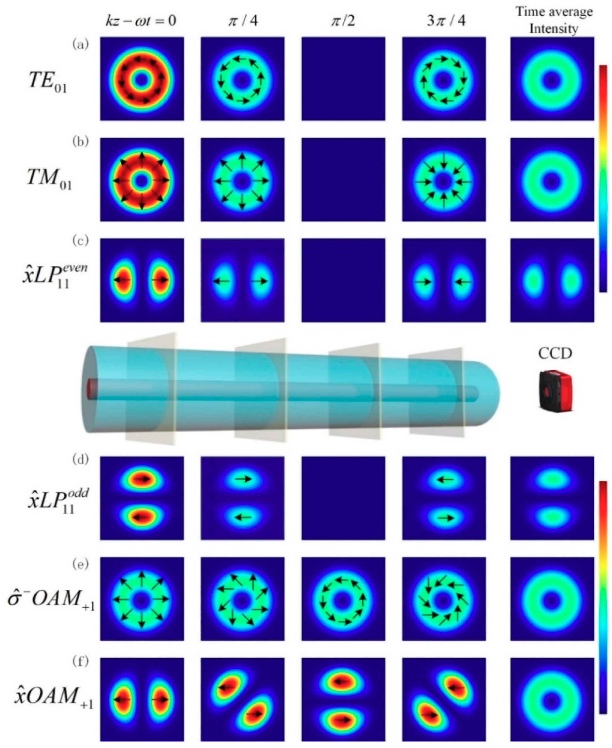
2.3. Orbital Angular Momentum Modes

OAM modes, are also one of the groups of fiber-based modes. Unlike the conventional plane light wave, OAM modes are characterized by a helical phase front $e^{\pm il\xi }$ [1], where ± l is the TC and $\xi$ is the azimuthal angle related to the optic axis. In addition, l can take the integer numbers from zero to $+\infty$. It should be noted that l is the same as the azimuthal order of CV modes. For different points on the beam cross-section with the same radius, the polarization states are the same, but with different phases. This indicates the helical phase front of OAM modes. Figure 2e,f show the propagating properties and time average intensity patterns of two typical OAM modes ${\widehat{\sigma }}^{-}OA{M}_{+1}$ and $\widehat{x}OA{M}_{+1}$. Taking ${\widehat{\sigma }}^{-}OA{M}_{+1}$ as an example, as indicated in Figure 2e, electric vectors at each point with the same radius on the beam cross section are the right-hand circular polarized (${\widehat{\sigma }}^{-}$). The phase factor of $OA{M}_{+l}$ should be $e^{i\left(kz-\omega t+l\xi \right)}$. For lth order OAM modes, the number of equal phase points on the beam cross section will be l. As shown in Figure 2e, initially, the x-polarization point is located at $\xi =0\left(kz-\omega t+\xi =0\right)$. Then, when the field propagates to $kz-\omega t=\frac{\pi }{4}$, the x-polarization point (with the same phase) is located at $\xi =-\frac{\pi }{4}\left(kz-\omega t+\xi =0\right)$. This means that, with $\xi =-\left(kz-\omega t\right)$, the equal phase point appears along the clockwise direction during the propagating, which indicates the factor $e^{i\xi }$. Thus, Figure 2e indicates ${\widehat{\sigma }}^{-}OA{M}_{+1}$ mode. The analysis method is similar to that of $\widehat{x}OA{M}_{+l}$. The symbol $\widehat{x}$ simply indicates the linear polarization, which can be substituted by another linear polarization symbol when the observation coordinates rotate.

For a typical combination of CV modes used to generate the OAM mode, ${\widehat{\sigma }}^{-}OA{M}_{+1}=T{M}_{01}-iT{E}_{01}$, as shown in Figure 2 The term “$-iT{E}_{01}$” indicates the figures of the first row (Figure 2a) with a $-\frac{\pi }{2}$ phase delay. The physical meaning of ${\widehat{\sigma }}^{-}OA{M}_{+1}=T{M}_{01}-iT{E}_{01}$ is the interference between $T{M}_{01}$ and $T{E}_{01}$ patterns with a $-\frac{\pi }{2}$ phase delay of $T{E}_{01}$. In Figure 2, when $T{M}_{01}$ propagates to $kz-\omega t=\frac{\pi }{2}$, $T{E}_{01}$ reaches $kz-\omega t=0$. Adding these two electric fields, we obtain the ${\widehat{\sigma }}^{-}OA{M}_{+1}$ at $kz-\omega t=\frac{\pi }{2}$. In addition to ${\widehat{\sigma }}^{-}OA{M}_{+1}=T{M}_{01}-iT{E}_{01}$, there are a series of transformation relations among CV, LP, and OAM modes. Moreover, we may note that there is no difference among the time average intensity patterns of CV and OAM modes. To further assure the phase information, a fundamental mode is usually used to interfere with a higher order fiber mode. Through the interference patterns we can obtain the phase information to confirm the specific electric vector field of the same doughnut intensity patterns. In the following section, we are going to derive the entire relation for CV modes, LP modes, and OAM modes, and introduce the generation and detection of OAM modes.

3. Basic Concepts and Theories of OAM Beams Generation and Detection

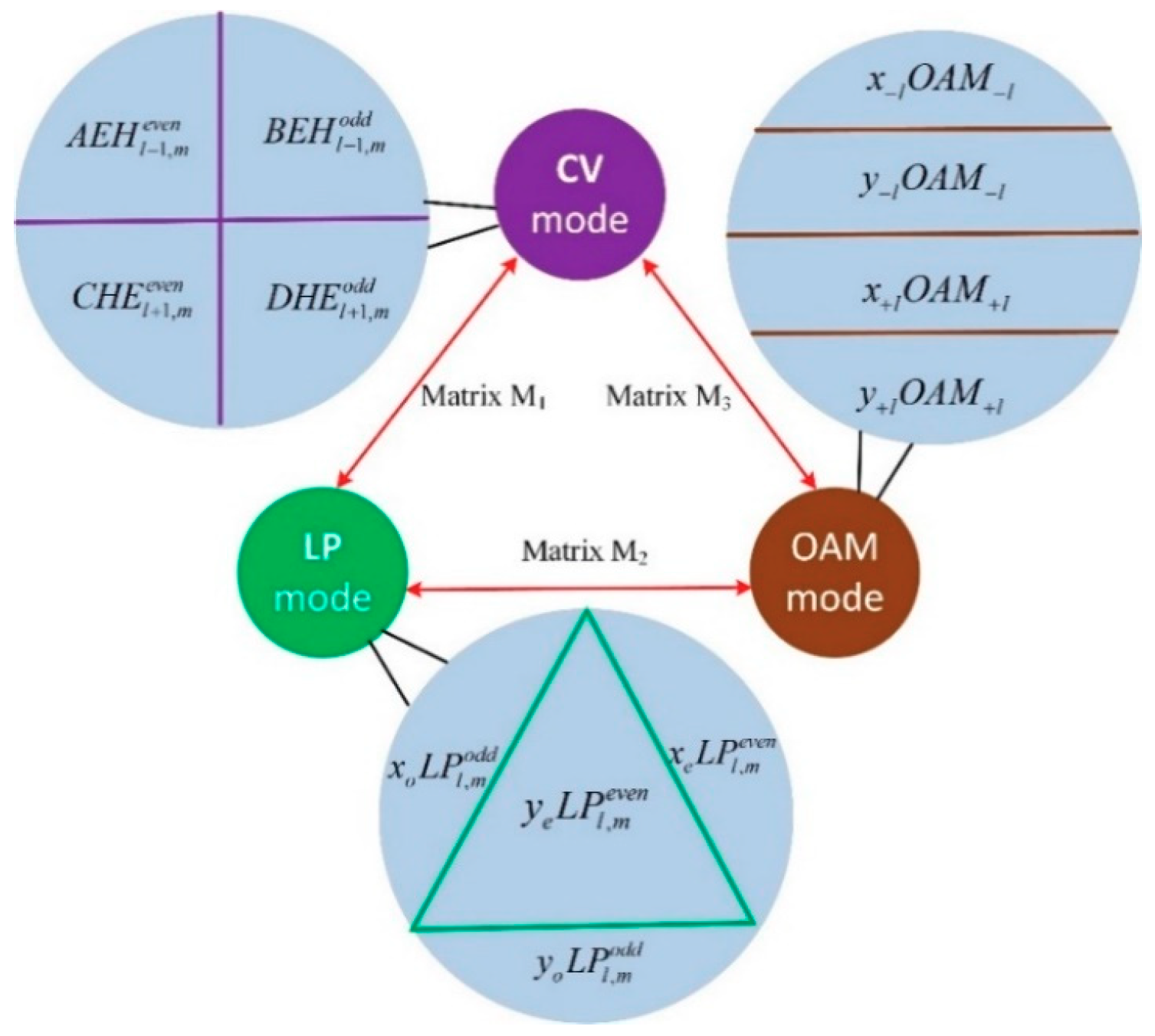
3.1. Transformation Relation among CV Modes, LP Modes, and OAM Modes

As the three groups of fiber mode bases, there is a transformation relation among CV modes, LP modes and OAM modes. Among these three modes, CV modes are the eigenmodes in fiber, which are able to propagate stably in fiber. We start our introduction of the transformation relation with CV modes.

In an axisymmetric index profile fiber, the intrinsic electric field is under the restriction of a cylindrical waveguide. By solving the Helmholtz equation in cylindrical coordinates, the eigenmodes in fiber can be derived, that is the CV modes. The solutions are given in Equation (1):

$$\left(\begin{array}{c}{E}_x(r,\xi ,z)\\ E_y(r,\xi ,z)\end{array}\right)=\{\begin{array}{cc}{F}_{l,m}(r)\left(\begin{array}{c}\cos (l\xi )\\ \sin (l\xi )\end{array}\right)e^{i{\beta }_{1}z};\hfill & \hfill E{H}_{l-1,m}^{even}/T{M}_{0,m}\hfill \\ F_{l,m}(r)\left(\begin{array}{c}-\sin (l\xi )\\ \cos (l\xi )\end{array}\right)e^{i{\beta }_{2}z};\hfill & \hfill E{H}_{l-1,m}^{odd}/T{E}_{0,m}\hfill \\ F_{l,m}(r)\left(\begin{array}{c}\cos (l\xi )\\ -\sin (l\xi )\end{array}\right)e^{i{\beta }_{3}z};\hfill & \hfill H{E}_{l+1,m}^{even}\hfill \\ F_{l,m}(r)\left(\begin{array}{c}\sin (l\xi )\\ \cos (l\xi )\end{array}\right)e^{i{\beta }_{4}z};\hfill & \hfill H{E}_{l+1,m}^{odd}\hfill \end{array}$$

(1)

where $\xi$ is the spatial angle, $F_{l,m}\left(r\right)$ is radial field distribution, l is the azimuthal order of CV modes, m is the radial order and β_1-4 are the propagation constants. Usually, $F_{l,m}\left(r\right)$ is the Bessel function in a step index fiber. For l = 1, $E{H}_{l-1,m}^{odd}$ should be substituted by $T{M}_{0,m}$ and $E{H}_{l-1,m}^{even}$ should be substituted by $T{E}_{0,m}$. In this section, however, we simply use $E{H}_{l-1,m}^{even}$ and $E{H}_{l-1,m}^{odd}$ to express the corresponding CV modes for conciseness, even for l = 1. Any lth-order electric field in fiber can be decomposed into the superposition of the four degenerated eigenmodes, that is, $E=AE{H}_{l-1,m}^{even}+BE{H}_{l-1,m}^{odd}+CH{E}_{l+1,m}^{even}+DH{E}_{l+1,m}^{odd}$, where ${\left(A,B,C,D\right)}^T$ is an arbitrary complex vector. The amplitudes and the phases of ${\left(A,B,C,D\right)}^T$ represent the amplitudes and the relative phases of $E{H}_{l-1,m}^{even},E{H}_{l-1,m}^{odd},\mathrm{and}H{E}_{l+1,m}^{even},H{E}_{l+1,m}^{odd}$, respectively.

In OAM mode bases, the four mode bases are $\widehat{x}OA{M}_{-l},\widehat{y}OA{M}_{-l},\widehat{x}OA{M}_{+l}$, and $\widehat{y}OA{M}_{+l}$, where $\widehat{x}\left(\widehat{y}\right)$ represents the $x$($y$) linearly polarized direction and $OA{M}_{\pm l}$ represents the OAM modes with TCs $\pm l$. With the aid of Jones calculus, any lth-order electric field can be expressed as $E=OA{M}_{-l}\left(\begin{array}{c}{x}_{-l}\\ y_{-l}\end{array}\right)+OA{M}_{+l}\left(\begin{array}{c}{x}_{+l}\\ y_{+l}\end{array}\right)$. Likely, as an arbitrary complex vector, ${\left(x_{-l},y_{-l},x_{+l},y_{+l}\right)}^T$ completely describes the entire lth-order electric field. In LP mode bases, the four mode bases are $\widehat{x}L{P}_{l,m}^{even},\widehat{y}L{P}_{l,m}^{even},\widehat{x}L{P}_{l,m}^{odd},\mathrm{and}\widehat{y}L{P}_{l,m}^{odd}$, where $L{P}_{l,m}^{even}$ and $L{P}_{l,m}^{odd}$ represent the two LP modes with complementary intensity patterns. Any lth-order electric field can be expressed in LP mode bases as $E=L{P}_{l,m}^{even}\left(\begin{array}{c}{x}_e\\ y_e\end{array}\right)+L{P}_{l,m}^{odd}\left(\begin{array}{c}{x}_o\\ y_o\end{array}\right)$. The corresponding complex vector is ${\left(x_e,y_e,x_o,y_o\right)}^T$.

For three groups of fiber mode bases, there exists transformation relation from CV modes to LP modes and OAM modes as follows (the detailed derivation can be found in [54]):

$$\frac{1}{2}\left(\begin{array}{cccc}1& -i& 1& i\\ i& 1& -i& 1\\ 1& i& 1& -i\\ -i& 1& i& 1\end{array}\right)\left(\begin{array}{c}A\\ B\\ C\\ D\end{array}\right)=\left(\begin{array}{c}{x}_{-l}\\ y_{-l}\\ x_{+l}\\ y_{+l}\end{array}\right)$$

(2)

for CV modes to OAM modes:

$$\left(\begin{array}{cccc}1& 0& 1& 0\\ 0& 1& 0& 1\\ 0& -1& 0& 1\\ 1& 0& -1& 0\end{array}\right)\left(\begin{array}{c}A\\ B\\ C\\ D\end{array}\right)=\left(\begin{array}{c}{x}_e\\ y_e\\ x_o\\ y_o\end{array}\right)$$

(3)

for CV modes to LP modes, and:

$$\frac{1}{2}\left(\begin{array}{cccc}1& 0& i& 0\\ 0& 1& 0& i\\ 1& 0& -i& 0\\ 0& 1& 0& -i\end{array}\right)\left(\begin{array}{c}{x}_e\\ y_e\\ x_o\\ y_o\end{array}\right)=\left(\begin{array}{c}{x}_{-}\\ y_{-}\\ x_{+}\\ y_{+}\end{array}\right)$$

(4)

for LP modes to OAM modes. If we define the transformation matrix of CV modes to LP modes (Equation (3)) as M₁, and the transformation matrix of LP modes to OAM modes as M₂ (Equation (4)), then the transformation matrix of CV modes to OAM modes (Equation (2)) is just the matrix product of M₁ and M₂, namely, M₃ = M₁M₂. Figure 3 shows the intuitive sketch describing the transformation relation among CV modes, LP modes and OAM modes. In Figure 3, the circle indicates all lth order electric fields, which should be a four-dimensional complex space, however, we simply use a two-dimensional circle to express them. The lines with different colors in the three circles indicate the different divided methods of the four-dimensional complex space. Notice that, the shapes of the lines are irrelevant. They are simply used to clearly denote the different space divided methods. Four degenerated modes operate as the different bases to completely describe the four-dimensional complex space (the entire lth order modes), where they can be transformed into each other through the transformation matrix derived above. The transformation among the mode bases is equivalent to the base transformation in the four-dimensional complex space, by the aforementioned matrices. The generation of pure OAM modes, is equivalent to adjust the mode field using physical methods to further simplify the expression in OAM mode bases. For example, a pure OAM mode $\widehat{x}OA{M}_{-l}$ expressed in OAM mode bases is ${\left(1,0,0,0\right)}^T$, whereas $0.5\left(E{H}_{l-1,m}^{even}+iE{H}_{l-1,m}^{odd}+H{E}_{l-1,m}^{even}-iH{E}_{l-1,m}^{odd}\right)$ or $0.5{\left(1,i,1,-i\right)}^T$ in CV mode bases and $\widehat{x}L{P}_{l,m}^{even}-i\widehat{x}L{P}_{l,m}^{odd}$ or ${\left(1,-i,0,0\right)}^T$ in LP mode bases. The three expressions denote the same spatial field which is not a pure CV mode or pure LP mode because the expression in the corresponding mode bases contain several components. The generation of pure CV modes or LP modes is similar.

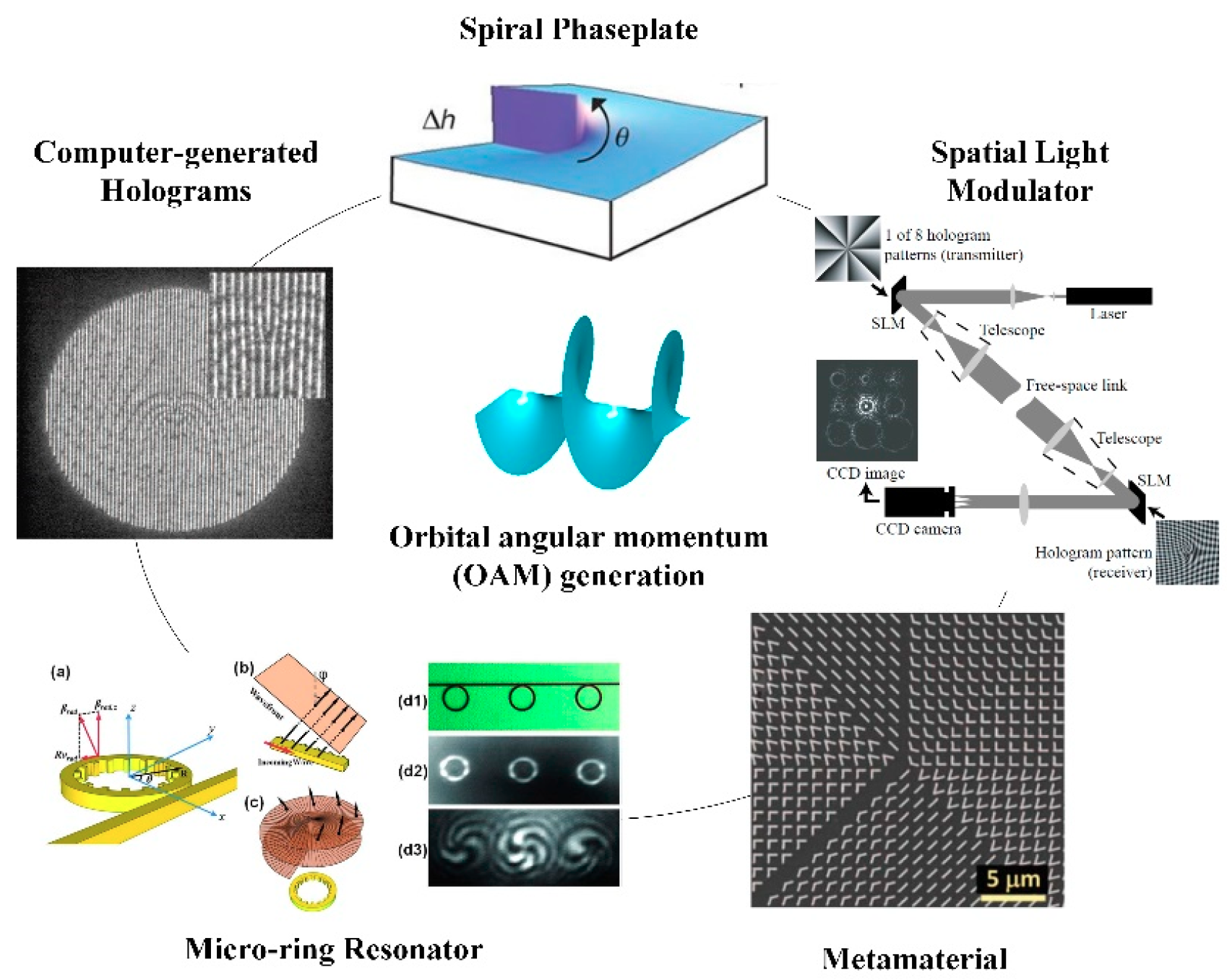
3.2. Generation of OAM Beams

Recently, all-fiber OAM generation methods have received increasing interests owing to the advantages of the lower insertion loss and better compatibility with the optical fiber communication links. The all-fiber system used to generate OAM beams can be summarized as shown in Figure 4. The system is divided into three parts: mode couple module, field control module, and polarization separation module.

Due to the difference of the effective refractive index (ERI) between different order modes being sufficiently large that mode coupling between different mode groups cannot occur by perturbations, such as fiber bending, twisting or extrusion. The mode couple module is used to couple the fundamental mode to a specific lth-order CV mode. It is usually composed of the fiber gratings [31,32,33,34,35,36,37,38,39,40,41,42,43,44] and the fiber couplers [45,46,47,48]. As mentioned above, the lth-order CV modes are composed of four degenerated modes. The mode couple module couples the fundamental mode to the lth-order CV modes, which can be seen as the superposition of the initial four degenerated modes with random amplitudes and phases in reality. This typically can’t be used to generate pure OAM beams.

The field control module, the polarization controller (PC) usually used in the fiber system, is applied to redistribute the generated random state of lth-order CV modes. Due to the ERIs of the four degenerated modes with the same order are approximately the same, the four degenerated modes with the same order will be strongly coupled to other degenerated modes in the same mode group when passing through the PC because of the bending, twisting, and extruding of the few-mode fiber (FMF) provided by the PC. This will change the relative amplitudes and phases among these four degenerated modes. In some particular situation, the pure OAM modes can be generated, such as ${\widehat{\sigma }}^{\pm }OA{M}_{\pm l}=H{E}_{l+1,m}^{even}\pm iH{E}_{l+1,m}^{odd}$.

The polarization separation module is used to separate two orthogonal polarized OAM modes after the polarization control module. It is composed of a QWP and a polarizer with a particular angle. The angle depends on the mode distribution prior to the polarization separation module. If the field control module generates an electric field of two orthogonal polarized OAM modes which carry different TCs, such as ${\widehat{\sigma }}^{+}OA{M}_{-l}+{\widehat{\sigma }}^{-}OA{M}_{+l}$, the two polarized orthogonal OAM modes can be separated through a polarization separation module. A polarization separation module is not necessary if the electric field after the polarization control module is carrying pure TC.

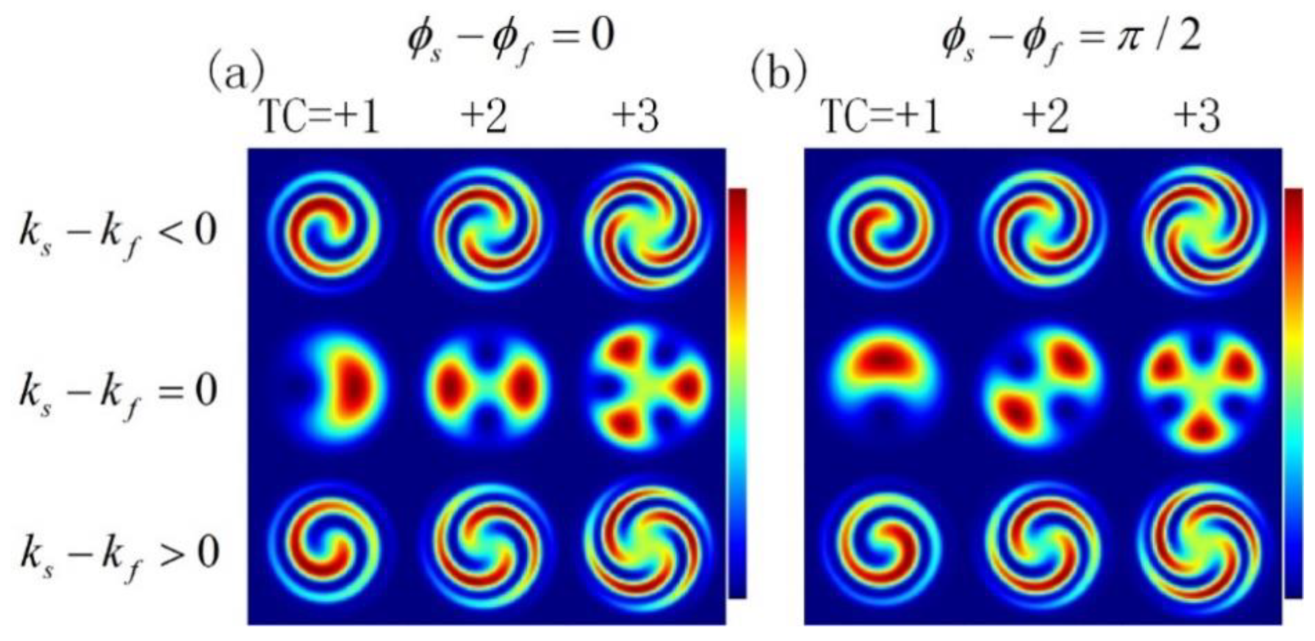
3.3. Detection of OAM Beams

Beams from the fiber will be converted into a divergent wave once they leave the fiber. For conciseness, we use a spherical wave to discuss the same physical process in this review. Indeed, they could be other types of divergent waves besides spherical waves, as long as their wavevectors are different from the other interference beam, such as a Gaussian light, whose curvatures of these lights are not the same on the beam cross-section when propagating while a spherical wave is a light wave with an invariant curvature. Without loss of generality, the physical meaning of the discussion below will not change under the assumption of a spherical wave.

The spherical wave is characterized by the factor $e^{ikR}$, where $k$ is the wavevector and $R={\left(x^2+y^2+z^2\right)}^{\frac{1}{2}}$ is the radius relative to the light source. A spherical wave carrying OAM TC = + l can be expressed as $E_s\left(r,\xi ,z\right)=F_{l,m}\left(r\right)e^{i\left(l\xi +k_s{\left(r^2+z^2\right)}^{\frac{1}{2}}\right)}$, where $k_s$ denotes the wavevector of OAM mode, $r={\left(x^2+y^2\right)}^{\frac{1}{2}}$ and $\xi$ denote the transverse radius and the spatial angle on the beam cross section respectively and $z$ denotes the propagating distance along with the optics axis. In addition, $F_{l,m}\left(r\right)$ is the radial field distribution, as mentioned above. A fundamental mode with a different divergence is usually used to interfere with OAM beam to detect the phase information of OAM beams. A spherical fundamental mode can be expressed as $E_f\left(r,\xi \right)=F_{0,1}\left(r\right)e^{i{k}_f{\left(r^2+z^2\right)}^{\frac{1}{2}}}$, where $k_f$ denotes the wavevector of fundamental mode. In general, the radial field distribution only affects the spot size but do not contribute to the final interference shapes. Herein, we omit the discussion about the radial field. Assume that the polarizations of the signal OAM beams and the interference beams are the same, the interference of the electric field should be:

$${\left|E\right|}^2={\left(E_s+E_f\right)}^{*}\left(E_s+E_f\right)={\left|E_s\right|}^2+{\left|E_f\right|}^2+E_s^{*}{E}_f+E_f^{*}{E}_s$$

(5)

where the left term ${\left|E_s\right|}^2+{\left|E_f\right|}^2$ is the direct current (DC) component invariant with the spatial angle $\xi$, which acts as an intensity base in the interference patterns. Because the DC component doesn’t affect the shapes of the patterns, we emphatically show the interference term $E_s^{*}{E}_f+E_f^{*}{E}_s$ through Equation (6):

$$E_s^{*}{E}_f+E_f^{*}{E}_s\propto F_{l,m}\left(r\right)F_{0,1}\left(r\right)\cos \left(l\xi +\left(k_s-k_f\right){\left(r^2+z^2\right)}^{\frac{1}{2}}+{\varphi }_s-{\varphi }_f\right)$$

(6)

where the term $F_{l,m}\left(r\right)F_{0,1}\left(r\right)$ indicates the area of interference related to the spot sizes of OAM beam and fundamental beam. Here, ${\varphi }_s-{\varphi }_f$ indicates the initial phase difference of OAM beam and the fundamental beam. Based on Equation (6), Figure 4 shows the interference patterns of $OA{M}_{+1}$, $OA{M}_{+2}$ and $OA{M}_{+3}$ with the different wavevector difference $k_s-k_f$ and initial phase difference ${\varphi }_s-{\varphi }_f$.

As can be seen, when $k_s\ne k_r$, the patterns exhibit the vortex shapes, while the vortex number indicates $\left|l\right|$, the absolute value of TC. Meanwhile, the vortex rotation direction is closely related to the difference between wave vectors of two beams. When $k_s-k_f<0$, which indicates that the fundamental beam is more divergent, a counter-clockwise vortex indicates l as the positive value while a clockwise vortex indicates the negative value. Contrary patterns exist when $k_s-k_f>0$. When $k_s=k_f$, the interference patterns do not exhibit the vortex shapes and we are unable to judge the specific TC for this type of interference.

Moreover, Figure 5a,b show the effects of the initial phase difference ${\varphi }_s-{\varphi }_f$ between the two interference beams on the interference patterns. When the initial phase difference changes, the patterns simply rotate an angle but do not change the number and direction of the vortex. This means that the initial phase difference does not disturb OAM beam detection under the interference condition.

If the physical process is angle-independent, the distinction between $OA{M}_{+l}$ and $OA{M}_{-l}$ is not important. We can simply define one direction of the rotated vortex as $OA{M}_{+l}$ and the other as $OA{M}_{-l}$. The counter-clockwise rotated vortex is usually defined as $OA{M}_{+l}$. However, if the physical process is related to the meta-surface, chiral devices, and some other angle-dependent devices, the distinction between $OA{M}_{+l}$ and $OA{M}_{-l}$ is crucial, and a meticulous method must be used, as discussed above. That is, the divergence of the signal OAM beam and the interference fundamental beam must be given.

Figure 6a shows another influencing factor in addition to the difference in wavevector, that is, the tilted degree, which indicates the difference in the propagating direction of the reference beam from the signal OAM beam. The larger the tilted degree is, the larger the angle of the propagating direction between the OAM beam and the reference beam. The effects of the TC and wavevector have been discussed above (Figure 5). Here, we highlight the effect of the tilted degrees. In Figure 6a, we set the propagating direction of the signal OAM beam as the reference axis (red arrow). On the top of Figure 6a, the red arrow indicates that the propagation direction of the signal OAM beam and the reference beam are the same. In addition, black arrows indicate the tilted degree between these two beams. As can be seen, the interference patterns shift into a fork-like shape from the vortex shape when the tilted degree increases. In addition, the open direction of the “fork” is closely related to the tilted direction. As shown in the second row in Figure 6a, for $OA{M}_{-1}$, the fork is upward open when the fundamental mode is left-tilted in relation to signal OAM beam. While it is downward open direction for a right-tilted fundamental mode. For $OA{M}_{+1}$ (the first row of Figure 6a), the results are opposite, compared to the first and the second rows in Figure 6a. Thus, interference patterns are closely related to the left-tilted or right-tilted between the OAM mode and the fundamental mode.

As for the effect of the difference of wavevectors, compared with the second and the fourth row of Figure 6a, the divergence (wavevector) difference $k_s-k_f$ does not disturb the judgement for nonzero tilted degree. Unlike a case of normal incidence (the middle red arrow), the vortex shape is different when the divergence difference $k_s-k_f$ changes, as shown in the middle column in Figure 6a, which will disturb the judgment about the TC of signal OAM beam. In addition, when disregarding TC = +l or TC = −l of the OAM mode, upward-open-fork shape patterns are usually defined as +l while the downward-open-fork shape patterns are defined as −l. Otherwise, it’s necessary to introduce the reference beam is left-tilted or right-tilted relative to the propagation direction of signal OAM beam.

In addition to using a fundamental beam with a different divergence to interfere with OAM beams, there are still some other methods to obtain the TC information of an OAM beam. The reference light $E_f$ can be other types, such as a tilted plane light wave and an OAM beam itself with a spatial translation. Without proof, we provide the typical interference patterns of these two types.

Figure 6b shows the interference between a non-divergent OAM beam ($OA{M}_{-1}$, $OA{M}_{-2}$ and $OA{M}_{-3}$) and right-tilted plane light wave ($k_s=k_f=0$). This is the degenerated case when $k_s-k_f=0$ and titled degree is non-zero in Figure 6a. We are able to judge different TCs through this interference method. In physical angle-independent processes, people generally define the number of interference line in the upper part l more than that in the lower part. In other words, a right-tilted reference beam is usually assumed if not caring about the sign of the TC. For an angle-dependent physical process, the tilted degree between the OAM mode and fundamental mode must be given.

As for Figure 6c, the OAM beam interferes with itself with a translation. If setting the propagating direction of the left-translational OAM beam as the reference axis (Figure 6a), the other OAM beam operates as a left-tilted reference beam related to the signal OAM beam. These two interference beams have the same divergence (wavevector). Thus, in the left area of arbitrary subfigure in Figure 6c, the TC is recognized as +l for a downward open fork-shaped pattern and −l for upward open fork-shaped pattern, according to the judging method given in Figure 6a. For the right area, the result is opposite, where the TC is +l for upward-opening-fork shape pattern and −l for downward-opening-fork shape pattern. To integrate these two methods, when comparing Figure 6b,c, we just need to focus on the right part in Figure 6c and use the same judgment process as that used for the tilted plane light wave (Figure 6b). In addition, the two rows patterns in Figure 6b,c show the effect of initial phase difference on the interference pattern. This simply leads to a translation of the patterns but not disturb the judgment about the TC.

4. Advances in Fiber OAM Generation Systems

4.1. Fiber Grating-Based OAM Generation Systems

Optical fiber gratings, a diffraction grating formed by the axially periodic refractive index modulation of fiber core using a certain method, have been developed into a mature technology and have been widely used in optical communications and fiber sensing in recent decades [55]. It is well-known that optical fiber gratings can be classified into two types, that is, fiber Bragg grating (FBG) [56] and long-period fiber grating (LPFG) [57,58,59,60,61,62,63,64,65,66,67,68], according to the grating period. The grating period of FBG is usually hundreds of nanometers or a few micrometers and the grating period of LPFG is usually hundreds of micrometers. In the FBG or LPFG, the fundamental mode in fiber core is coupled to the backward- or forward-propagating cladding mode or core mode at distinct wavelengths respectively. LPFG, written into a few-mode fiber, is the most commonly used an OAM conversion device. The working principle of the LPFG is the coupled mode theory. When the grating period satisfies the phase-matching condition λ_m = (n_eff1 − n_eff2)Λ, where λ_m is the resonant wavelength, n_eff1 and n_eff2 are the effective refractive index (ERI) of fundamental mode and higher-order core mode, respectively, the fundamental mode in the fiber core will be coupled to higher-order core mode, thereby leading to the transmission spectrum of the fundamental mode with one or a few notches, as shown in Figure 7c.

There have been several methods used to fabricate an LPFG, including ultraviolet laser [57], femtosecond laser irradiation [58], CO₂ laser irradiation [27,32,43,59,60,61], cleaving-splicing method [62], arc discharge [63], acousto-optic interaction [64], mechanical micro-bending [31,33,34,35,65], and so on. The CO₂ laser irradiation and mechanical micro-bending are the two frequently-used methods to fabricate the LPFG to generate the OAM modes.

The working principle of the mechanically induced LPFG is shown in Figure 7a. The few-mode fiber is placed between two plates with periodically grooves or between a plate with periodically grooves and a flat plate. When the period satisfies the phase-matching condition and putting pressure on the one of the two plates, the fundamental mode will be coupled to the higher-order core mode. The advantages of this method are that one can adjust the resonant wavelength or the order of coupled higher order mode, by adjusting the grating period. In addition, the length of the fiber under pressure, which controls the linewidths of the notch, can easily be changed. In addition, the depth of the notches can be tuned by adjusting the pressure. Finally, when the pressure is removed, the transmission spectrum of the fiber returns to its initial spectrum. The disadvantage of this method is some fiber cannot be used to fabricate an LPFG.

Compared with the methods mentioned above, a high-frequency CO₂ pulse is an attractive tool used to fabricate an LPFG owing to its convenience, economy and high efficiency. As shown in Figure 7b, the CO₂ laser irradiation method uses a high-frequency CO₂ laser to continuously notch grooves on one side of the few-mode fiber to form a series of periodic structures. Because of the advantages of a CO₂ laser writing technique, the LPFGs can be successfully written into various types of special fiber, such as multi-core fiber [66] and photonic crystal fiber [61,67], and different types of LPFG, such as a sampled or a chirped grating, can be inscribed in the fiber [68]. However, this method has broken the fiber structure, and the resonant wavelength and the coupled mode are fixed once the LPFG is fabricated.

In general, fiber grating-based methods for pure OAM mode generation, with experimental set up as shown in Figure 8a, can be classified into two types according to the source modes. For one type, the OAM modes can be generated by combining two linearly polarized modes with a π/2 phase shift, where the generated OAM modes have no spin angular momentum (SAM). For the other type, the OAM modes can be generated by combining two vector modes ($H{E}_{l+1,m}$ or $E{H}_{l-1,m}$) with a π/2 phase shift, where the generated OAM modes have the SAM at the same time. There have been many reports about the generation of these two types OAM modes using LPFGs [32,34,35,37,43].

For the first type, namely the generation of linearly-polarized OAM (LP-OAM) modes, the LP-OAM modes in the x and y polarized directions can be obtained by eliminating other component in the OAM mode bases except one, such as ${\left(x_{-l},y_{-l},x_{+l},y_{+l}\right)}^T={\left(1,0,0,0\right)}^T$, which corresponds to $\widehat{x}OA{M}_{-l}$, an x-linear polarized OAM beam with TC = +l. The expression in other mode bases can be obtained by substituting this vector into Equation (2) or Equation (4). ${\left(x_{-l},y_{-l},x_{+l},y_{+l}\right)}^T={\left(1,0,0,0\right)}^T$ is equivalent as ${\left(A,B,C,D\right)}^T=0.5,0.5i,0.5,-0.5i^T$ and ${\left(x_e,y_e,x_o,y_o\right)}^T={\left(1,0,-i,0\right)}^T$. Given a physical meaning, that is $\widehat{x}OA{M}_{-l}=0.5E{H}_{l-1,m}^{even}+0.5iE{H}_{l-1,m}^{odd}+0.5H{E}_{l+1,m}^{even}-0.5iH{E}_{l+1,m}^{odd}=\widehat{x}L{P}_{l,m}^{even}-i\widehat{x}L{P}_{l,m}^{odd}$. Thus, the LP-OAM can be obtained by combining the even and odd $L{P}_{l,1}$ mode having the same polarized direction with a ±π/2 phase shift. The first order LP-OAM modes, composed of $L{P}_{11}^a$ and $L{P}_{11}^b$ mode with a π/2 phase shift, using a two-mode fiber (TMF), a mechanical LPFG, a mechanical rotator and metal slabs, as shown in Figure 8a, and the second order LP-OAM modes, composed of $L{P}_{21}^a$ and $L{P}_{21}^b$ mode with a π/2 phase shift, utilizing an LPFG written in a four-mode fiber induced by CO₂ laser irradiation, have been experimentally demonstrated in [35] and [37], respectively.

For the other type, namely the generation of circularly-polarized OAM (CP-OAM) modes, the typical CP-OAM modes with SAM being ±1 can be obtained by the following equation [43]:

$$\begin{array}{l}\left(\begin{array}{l}{\widehat{\sigma }}^{-}OA{M}_{+1}\\ {\widehat{\sigma }}^{+}OA{M}_{-1}\\ {\widehat{\sigma }}^{+}OA{M}_{+1}\\ {\widehat{\sigma }}^{-}OA{M}_{-1}\end{array}\right)=F_{1,1}(r)\left(\begin{array}{cccc}1& i& 0& 0\\ 1& -i& 0& 0\\ 0& 0& 1& i\\ 0& 0& 1& -i\end{array}\right)\left(\begin{array}{l}H{E}_{21}^{even}\\ H{E}_{21}^{odd}\\ T{M}_{01}\\ T{E}_{01}\end{array}\right),l=1\\ \left(\begin{array}{l}{\widehat{\sigma }}^{-}OA{M}_{+l}\\ {\widehat{\sigma }}^{+}OA{M}_{-l}\\ {\widehat{\sigma }}^{+}OA{M}_{+l}\\ {\widehat{\sigma }}^{-}OA{M}_{-l}\end{array}\right)=F_{l,1}(r)\left(\begin{array}{cccc}1& i& 0& 0\\ 1& -i& 0& 0\\ 0& 0& 1& i\\ 0& 0& 1& -i\end{array}\right)\left(\begin{array}{l}H{E}_{l+1,1}^{even}\\ H{E}_{l+1,1}^{odd}\\ E{H}_{l-1,1}^{even}\\ E{H}_{l-1,1}^{odd}\end{array}\right),l\ge 2\end{array}$$

(7)

where ${\widehat{\sigma }}^{+}$ and ${\widehat{\sigma }}^{-}$ represent left- and right-handed circular polarization. Taking ${\widehat{\sigma }}^{+}OA{M}_{+1}$ as an example, one can just set the expression in the OAM mode bases as ${\left(x_{-l},y_{-l},x_{+l},y_{+l}\right)}^T={\left(0,0,1,i\right)}^T$ and calculate the corresponding expression in the CV mode bases or LP mode bases, the results of which are the same as Equation (7). The first- and second-order CP-OAM modes composed of even and odd $H{E}_{21}$, $H{E}_{31}$, $E{H}_{11}$ and $T{M}_{01}$, $T{E}_{01}$ modes with a π/2 phase shift are experimentally demonstrated in [43] by our group, as shown in Figure 8b,c, using two LPFGs written in a four-mode fiber induced by CO₂ laser. The first LPFG is used to convert fundamental mode to the first order mode. The second LPFG is used to convert the generated the first order mode to the second order mode which has wider bandwidth than the LPFG converting fundamental mode to the second order mode.

The OAM mode generated mentioned above is only one pure OAM mode with the same polarization. There are other two types of mixed OAM modes composed of two orthogonal polarized OAM modes with the opposite TCs, according to the polarization state of the two orthogonal modes that can be generated in all-fiber system. One type is LP-OAM, while the other type is CP-OAM.

For the first type, the mixed OAM mode, composed of two orthogonal LP-OAM modes with the opposite TCs, can be obtained by the following equation:

$$E=\{\begin{array}{l}E{H}_{l-1,1}^{even}\pm iH{E}_{l+1,1}^{odd}=\widehat{x}OA{M}_{\pm l}\pm i\widehat{y}OA{M}_{\mp l}\\ E{H}_{l-1,1}^{odd}\mp iH{E}_{l+1,1}^{even}=\widehat{x}OA{M}_{\mp l}\pm i\widehat{y}OA{M}_{\pm l}\end{array}$$

(8)

where E represents the mixed OAM mode. We can find that the mixed OAM modes are composed of x- and y-polarized LP-OAM modes with the opposite TCs, and these two orthogonal LP-OAM modes can be separated by a polarizer. In 2016, Jiang et al. experimentally demonstrated a method to generate optical vortices with tunable OAM in optical fiber by using a mechanical LPFG, a mechanical rotator and a metal parallel slab [34]. The tunable OAM mode can be seen as a combination of $H{E}_{l+1,m}^{even}$ ($H{E}_{l+1,m}^{odd}$) and $E{H}_{l-1,m}^{odd}$ ($E{H}_{l-1,m}^{even}$), with a π/2 phase shift. They experimentally achieved the smooth variation of OAM mode from l = −1 to l = +1 by adjusting the polarizer placed at the end of the fiber, as shown in Figure 8d.

For the other type, the mixed OAM mode, composed of two orthogonal CP-OAM modes with the opposite TCs, can be obtained by the following equation:

$$\begin{array}{l}E{H}_{l-1,m}^{even}=\frac{1}{2}\left({\sigma }^{-}OA{M}_{-l}+{\sigma }^{+}OA{M}_{+l}\right)\\ E{H}_{l-1,m}^{odd}=-\frac{i}{2}\left({\sigma }^{-}OA{M}_{-l}-{\sigma }^{+}OA{M}_{+l}\right)\\ H{E}_{l+1,m}^{even}=\frac{1}{2}\left({\sigma }^{+}OA{M}_{-l}+{\sigma }^{-}OA{M}_{+l}\right)\\ H{E}_{l+1,m}^{odd}=\frac{i}{2}\left({\sigma }^{+}OA{M}_{-l}-{\sigma }^{-}OA{M}_{+l}\right)\end{array}$$

(9)

We can see that the arbitrary single CV mode can be seen as a linear combination of a left-handed and a right-handed CP-OAM with the opposite TC. Since one of these two CP-OAM is left-handed, the other one is right-handed, we can use a QWP to make these two CP-OAM have an orthogonal projection. Then we can use a polarizer with optical axis rotating to one projection orientation to filter out the other CP-OAM. The authors of this paper have experimentally demonstrated that using a single CV mode in a two-mode fiber (TMF), the topological charge of generated OAM mode can be switched among −1, 0, +1, as shown in Figure 8e [32]. In our work, a CO₂-laser induced rocking LPFG inscribed in the two-mode fiber is fabricated to efficiently generate the CV mode, including $T{E}_{01}$, $T{M}_{01}$ and $T{E}_{01}\pm T{M}_{01}$ mode. Then a QWP and a polarizer are used to separate the two CP-OAM modes.

The OAM modes obtained by [34,35,37,43] are all generated by a combination of two or four degenerated modes in the same mode group and the associated eigenmodes must maintain a stable phase and polarization. In addition, in ideal cylindrical waveguides such as fiber, the propagation constants of the $T{E}_{01}$ and $T{M}_{01}$ mode are different. For example, the effective index separation between the $T{E}_{01}$ and $T{M}_{01}$ mode is measured to be 6.6 × 10⁻⁴ in the fiber [36]. The purity of CP-OAM generated by combination of $T{M}_{01}\pm iT{E}_{01}$ or $H{E}_{21}^{even}\pm iT{E}_{01}$ cannot be maintained when the length of optical fiber is changed. However, the OAM modes generated by a single CV mode don’t have this problem.

However, the generated OAM modes obtained by the studies mentioned above are dependent on the polarization state of the input light, namely, these all-fiber generators exhibited a sensitivity requiring specialized polarization states for the input light without adjusting the PC. Zhang et al. have proposed a polarization-independent OAM generator based on a chiral fiber grating (CFG) fabricated by twisting a fused few-mode fiber during hydrogen-oxygen flame heating [44]. They experimentally fabricate a left-handed CFG (LCFG) and a right-handed CFG (RCFG) to convert the fundamental mode to the OAM mode, and experimentally investigate the polarization characteristics, helical phase of the coupled mode in CFG for varying polarization state of input light. Their results showed that the coupled OAM mode had the same polarization state with the input fundamental mode. And the chirality of the generated OAM mode was polarization-independent and determined solely by the helicity of the CFG, as shown in Figure 9. The OAM mode generated by the RCFG can only be $OA{M}_{+1}$ mode, while OAM mode generated by the LCFG can only be $OA{M}_{-1}$ mode.

Compared to other mode converters, LPFGs have many advantages, such as low loss, small size, easy fabrication, and high coupling efficiency up to 99%, and so on. However, LPFGs also have many disadvantages compared with the mode selective coupler and the photonic lantern, for example, the narrow bandwidth and one LPFG can only convert the fundamental mode (the zeroth order mode) to a phase-matching higher order mode. Thus, there have been many attempts to increase the bandwidth of an LPFG, such as chirped LPFG [69], length-apodized LPFG [70], the cascading of several LPFGs [43], operating an LPFG at its turning point along its phase-matching curve [71], shortening the length of the LPFG, namely decreasing the number of grooves [72], and so on. However, chirping can significantly decrease the mode conversion efficiency and the bandwidth increase is still limited. For LPFG operating at its turning point, such a turning point may not exist for a given set of guided modes. For shortening the length of LPFG, it will decrease the coupling efficiency. For the cascading of several LPFGs, for example, the bandwidth of cascading two LPFGs that one LPFG convert fundamental mode to the first order mode and the other LPFG convert the first order mode to the second order mode is wider than the bandwidth of LPFG that directly converts fundamental mode to the second order mode [43], However, this method needs the fabrication of several LPFGs, which brings about extra loss.

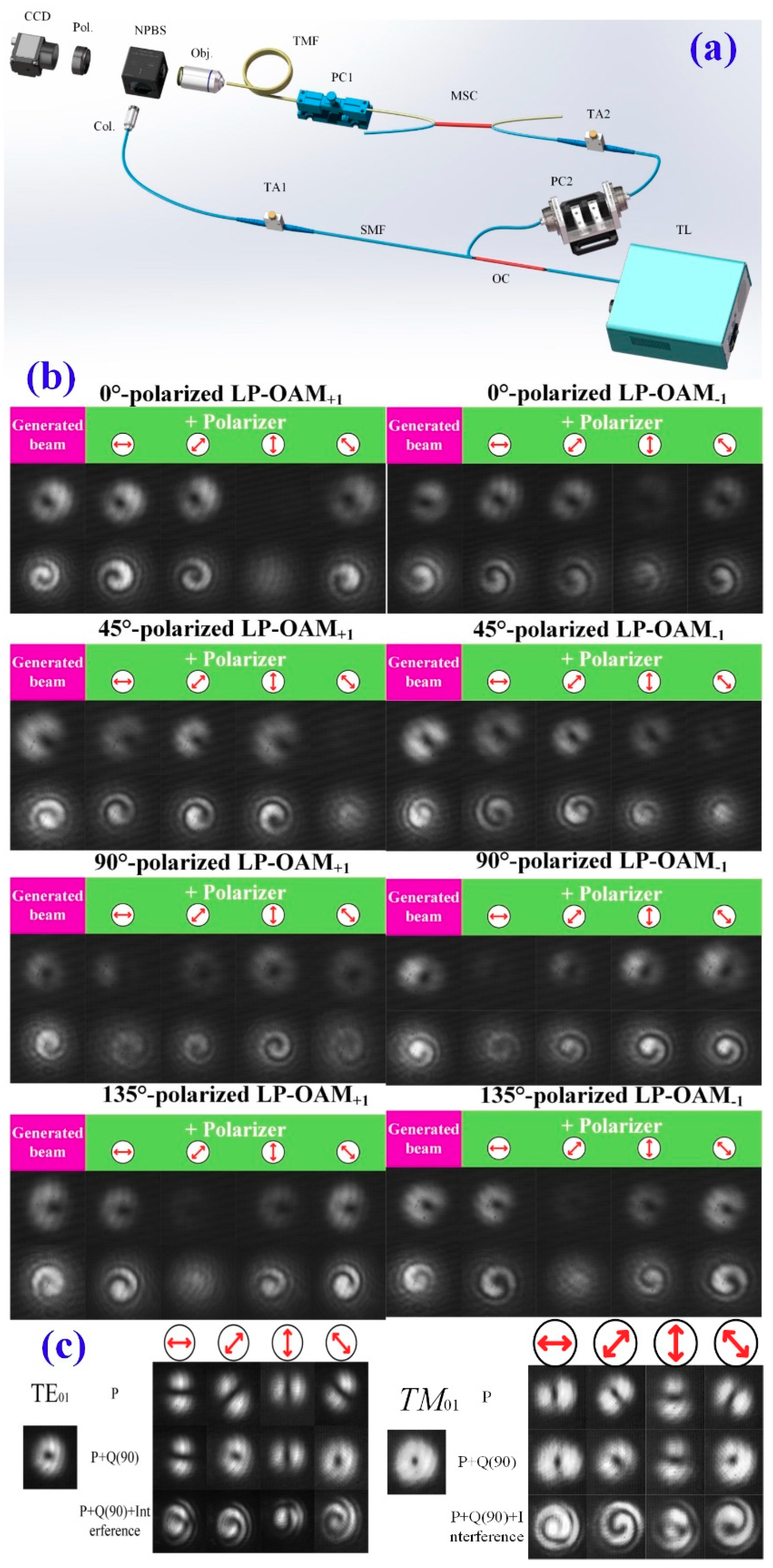
4.2. Mode Selective Coupler (MSC)-Based OAM Generation Systems

Optical fiber couplers have been widely used in many research areas, such as optical communication, optical sensing, and fiber lasers. In addition, the fiber couplers can be fabricated from various types of fibers, such as single mode fiber, few mode fiber, polarization-maintaining fiber, and ring core fiber.

The operation principle of the MSC is shown in Figure 10. Composed of SMF and FMF, MSC is based on the phase-matching condition between the fundamental mode in the SMF and higher order modes in the FMF. This can be achieved by satisfying the ERI of the fundamental mode in the SMF equaling to that of the higher order mode in the FMF. When the phase-matching condition is satisfied, the fundamental mode in the SMF will be converted to the particular higher order mode in the FMF.

In order to determine the coupling efficiency between the fundamental mode and high-order modes on the fiber tapering diameter, the following coupled equations are solved [73]:

$$\begin{array}{l}\frac{d{A}_1(z)}{dz}=i\left({\beta }_1+C_{11}\right)A_1+i{C}_{12}{A}_2\\ \frac{d{A}_2(z)}{dz}=i\left({\beta }_2+C_{22}\right)A_2+i{C}_{21}{A}_1\end{array}$$

(10)

where z is the distance along the coupling region of the MSC, A₁ and A₂ are the slowly-varying field amplitudes in the SMF and FMF of the MSC, and β₁ and β₂ are the propagation constant of fundamental mode in the SMF and higher order mode to be coupled in the FMF, respectively. Due to the phase matching condition that ERI of fundamental mode in the SMF equaling to that of the first or second order modes in the FMF, β₁ should be equal to β₂. C₁₁ and C₂₂, C₁₂, and C₂₁ are the self-coupling and mutual coupling coefficients, respectively. Self-coupling coefficients are small relative to mutual coupling coefficients, and can be ignored. Moreover, the mutual coupling coefficients C₁₂ ≈ C₂₁ ≈ C, where C is a coefficient depending on the width and length of the coupling region. Thus, the power distribution in coupler can be given as follows [74]:

$$\begin{array}{l}{P}_1(z)={\left|A_1(z)\right|}^2=1-F^2{\sin }^2(\frac{C}{F}z)\\ P_2(z)=F^2{\sin }^2(\frac{C}{F}z)\end{array}$$

(11)

where $F={\left(1+\frac{{\beta }_1-{\beta }_2}{4C^2}\right)}^{-\frac{1}{2}}$, F² is the maximum coupling power between two fibers. According to Equation (11), it can be found that the power in coupling region exchanges periodically.

The MSC can be divided into two types according the fiber type used in its fabrication. One type is the MSC composed of the SMF and the FMF or multimode fiber (MMF). The FMF and MMF are similar to the SMF, which is composed of a core, cladding, and coating. The RI difference between the fiber core and cladding or the radius of the fiber core of FMF/MMF is larger than that of SMF. The other type is the MSC composed of the SMF and the ring core fiber (RCF), also called vortex fiber. The RCF is usually composed of three parts, namely, the fiber core, cladding, and ring. In these three parts, the RI of the ring is the highest. Thus, the light is able to be restricted and propagate in the ring. While it’s invariant for the RI of the fiber core and cladding. The RCF can limit the radial order m to 1 and thereby fix the number of degenerated modes in each high azimuthal order mode group to be 4, which will decrease the multi-input-multi-output complexity. In addition, the RCF is more suitable for transmitting OAM modes than the FMF or MMF. However, the fabrication of RCFs is more difficult than the FMF/MMF. The fabrication of MSC, composed of SMF and the FMF/MMF is easier than the MSC composed of SMF and RCF, while the later MSC is more compatible to the OAM mode transmission system than the MSC composed of FMF/MMF. There have been many works to generate OAM mode based on the two types of MSCs [45,46,47,48]. The experimental setup usually used to generate the OAM mode based on the MSC is shown in Figure 11a The MSC is used to couple the fundamental mode to the higher order CV mode group, and the polarization controllers are used to redistribute the generated random state of lth-order CV modes to the OAM modes we want to obtain. The polarizer is used to identify the polarization state of the generated OAM modes or to separate the two orthogonal OAM modes.

The authors of this paper have also experimentally demonstrated that arbitrary linearly-polarized OAM mode can be generated by carefully adjusting the PC without changing the polarization state of the input light based on the MSC, composed of a SMF and a TMF. The experimental results are shown in Figure 11b. We can find that the 0°-, 45°-, 90°-, and 135°-polarized LP-OAM modes with $\pm 1$ TC are generated successfully. In addition, we have also experimentally demonstrated the generations of ${\sigma }^{+}OA{M}_{\pm 1}$ and ${\sigma }^{-}OA{M}_{\pm 1}$ mode using a single first order CV mode, including $T{M}_{01}$, $T{E}_{01}$, $H{E}_{21}^{even}$, and $H{E}_{21}^{odd}$ modes. These two CP-OAM modes can be separated by using a QWP and a polarizer with an angle ±π/4. The results are shown in Figure 11c.

Yao et al. have proposed an all-fiber system to generate tunable first order OAM mode based on an all-fiber MSC, composed of an SMF and a TMF [48]. The MSC is used to couple fundamental mode to the first order mode. And they experimentally demonstrate the generation of first order OAM mode, produced by combining $H{E}_{21}^{even}$ and $T{E}_{01}$ (or $H{E}_{21}^{odd}$ and $T{M}_{01}$) with a π/2 phase shift, and the topological charge of generated OAM mode can be tuned from −1 to +1 by adjusting the polarizer placed at the end of the FMF.

The excitation of first order CP-OAM modes obtained by Equation (7), using an MSC composed of an SMF and an RCF for the first time have been experimentally demonstrated in [47], and the mode purity of excited OAM mode is up to 75%.

Compared to the fiber grating-based mode converters mentioned above, the advantages of MSC include low loss, small size, easy fabrication, broad-bandwidth and the controllable coupling efficiency for the pure high-order mode which can be used in certain situations, such as in laser cavities, and so on. However, the MSCs also have disadvantages, for example, one MSC can only convert the fundamental mode to a particular high-order mode and, thus, we can only obtain one OAM mode by one MSC. If we want to multiplex N OAM modes, we need to cascade N MSCs which brings extra loss and complexity.

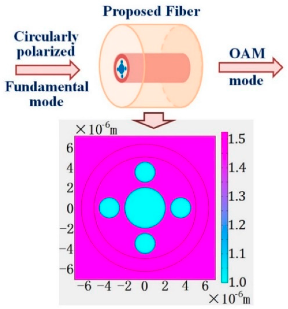
4.3. Micro-Structured Optical Fiber-Based OAM Generation System

The generation of OAM mode by the studies mentioned above are based on the all-fiber system concluded in Figure 4. The mode coupling module can only couple the fundamental mode to the mixed mode composed of four degenerated modes in the lth-order CV mode group with random phase and amplitude. A field control module is used to redistribute the phase and amplitude of four degenerated modes to generate the OAM mode. It is usually difficult to obtain one particular OAM mode by adjusting the PC in the all-fiber system. It is more convenient if we can use a special fiber device to directly couple the fundamental mode to the OAM mode we want. There have been some reported works generating OAM modes directly through a special micro-structured optical fiber design [49,50,51].

There are two main operating principles of designing fiber for converting the fundamental mode to the high order OAM modes. One is based on the mode coupling theory. The designed fibers based on this principle are usually composed of one or several single-mode cores used to support the fundamental mode and one ring core used to support OAM mode. The electric fields of the fundamental core mode and the high order mode in the ring can be expressed as:

$$\begin{array}{l}{E}_A\left(r\right)=A\left(z\right)E_A\left(x,y\right)\exp \left(i{\beta }_{A}z\right)\\ E_B\left(r\right)=B\left(z\right)E_B\left(x,y\right)\exp \left(i{\beta }_{B}z\right)\end{array}$$

(12)

where the coefficients A(z) and B(z) vary with z. And according to coupling mode theory, the two coefficients satisfy:

$$\begin{array}{l}\frac{dA\left(z\right)}{dz}=i{\kappa }_{AA}A+i{\kappa }_{AB}B{e}^{i({\beta }_B-{\beta }_A)z}\\ \frac{dB\left(z\right)}{dz}=i{\kappa }_{BB}B+i{\kappa }_{BA}A{e}^{i({\beta }_A-{\beta }_B)z}\end{array}$$

(13)

The mode coupling coefficient κ is given by:

$${\kappa }_{\upsilon \mu }=\frac{\omega }{4}{\displaystyle \underset{-\infty }{\overset{\infty }{\int }}{\displaystyle \underset{-\infty }{\overset{\infty }{\int }}{E}_{\upsilon }^{*}(x,y)\cdot \Delta \epsilon \cdot E_{\mu }\left(x,y\right)}}dxdy$$

(14)

where ω is the optical frequency, and △ε is the perturbation to the permittivity. The light power is supposed to only be launched into the fundamental mode core, so the coupling mode equation can be solved as:

$$\begin{array}{l}A\left(z\right)=(\cos \gamma z-\frac{i\delta }{\gamma }\sin \gamma z)e^{i\delta z}\\ B\left(z\right)=\left(\frac{i{\kappa }_{BA}}{\gamma }\sin \gamma z\right)e^{-i\delta z}\end{array}$$

(15)

where γ = (κ_AB × κ_BA + δ²)^1/2 and δ is the phase mismatching coefficient, where, δ = (β_B + κ_BB − κ_AA − β_A)/2. The mode coupling efficiency can be expressed as:

$$\eta =\frac{{\left|{\kappa }_{BA}\right|}^2}{{\gamma }^2}{\sin }^2\gamma z$$

(16)

The authors of this paper have proposed and investigated a tunable microstructure optical fiber for different OAM mode generation by simulation based on the mode coupling theory. The microstructure optical fiber is composed of a high RI ring and a hollow core surrounded by four small air holes as shown in Figure 12 [49]. The hollow core and the surrounded four air holes are infiltrated by optical functional material whose RI can be modulated by physical parameters, leading to conversion between circularly-polarized fundamental mode and different OAM mode in the high RI ring with tunable operating wavelengths. The OAM modes are composed by ${\widehat{\sigma }}^{\pm }OA{M}_{\pm l,1}=H{E}_{l+1,1}^{even}\pm iH{E}_{l+1,1}^{odd}$ and ${\widehat{\sigma }}^{\mp }OA{M}_{\pm l,1}=E{H}_{l+1,1}^{even}\pm iE{H}_{l+1,1}^{odd}$, where l ranges from 2 to 8.

The other is to mimic the refractive spiral phase element [50,51]. This method typically uses the multi-core fiber (MCF) [50] or photonic crystal fiber (PCF) [51]. For the MCF, the phase change is a function of the core RI. Therefore, by arranging the RI distribution among the multi cores of the MCF. The phase difference between the adjacent core exactly equal 2πl/N where l is the TC of the desired OAM mode and N is the number of cores of MCF. With such a phase difference distribution, when the spatial-phase-modulated multi-beams converge in a section of ring core fiber (RCF), the OAM mode with TC l can be effectively generated [50]. For PCF, the air-holes in silica are arranged for the transverse subwavelength grating in [51]. The air-hole diameter across the transverse dimension can be varied to create an arbitrary ERI profile N_eff(r, θ) = N₀ + △N_eff(r, θ), where N₀ and △N_eff(r, θ) are the constant and varying parts of N_eff(r, θ). To generate OAM with TC l, the introduced ERI perturbation △N_eff(r, θ) must satisfy the phase-matching condition:

$$\Delta N_{eff}(r,\theta )=l\frac{\lambda }{z}\frac{\theta }{2\pi }$$

(17)

where z is the length of the PCF.

The OAM generation methods based on the fiber design not only have the advantages of the fiber device such as low loss and small size, but also have the advantages such as directly converting the fundamental mode to the OAM mode and the TCs of generated OAM being controllable. However, the structures of the designed fiber are usually complicated and difficult to fabricate in reality.

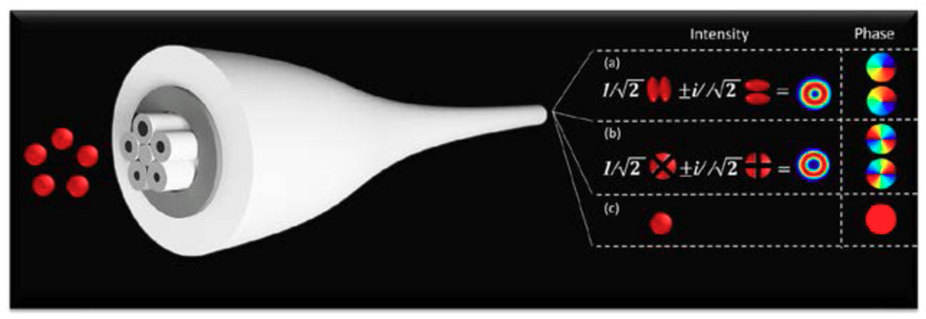
4.4. OAM Generation Based on Photonic Lantern

The photonic lantern (PL) is a low-loss optical device that connects several single-mode cores or few-mode cores to a single multimode core. Early interest in PLs were based on their original application in astronomical instrumentation [75,76], but recently its application in optical fiber communication has been attracting increased attention from researchers. The PL can be a spatial multiplexer for space-division multiplexing because one PL can multiplex N modes where N is the number of SMF used to fabricate the PL, which in principle allows the capacity of the communication system to be multiplied by N [77,78,79,80,81,82,83,84,85,86,87,88,89].

There are five types of PLs that have been reported to date [80,81,82,83,84,85,86,87,88,89,90]. The first type of PLs is fabricated by inserting N separate SMFs into a surrounding glass cane which is usually the PCFs made from glass with a pattern of air holes in the cladding [80,81]. Then the resulting glass body is heated and drawn down to form a taper transition to an MMF port. The MMF core is formed by the fused mass of SMFs, with the reduced-index cladding formed by the cane glass. This method has the advantages of easy control of the arrangement of SMFs by designing the arrangement of air holes of the cane. However, the SMFs are accommodated in separate compartments. The second type of PLs is fabricated by inserting a bundled N SMFs together into a capillary which has a lower RI than that of the SMF cladding [82,83]. Then the capillary is heated and drawn on a tapering machine to form the MMF port, which is more practical. However, the arrangement of SMFs with this method is more difficult than that of the first type of PLs, and with the number of SMFs increasing, the difficulty of fabricating PLs also increases. The third type of PLs is fabricated by inserting an MCF into a capillary which has a lower RI than that of the MCF cladding [84,85]. Then the capillary is heated and drawn on a tapering machine to form the MMF port. This method has the advantages, for example, several kilometers of the MSC can be drawn at once and this method needs only one MCF compared to the first and second type of PLs needing N SMFs. However, the MCF used in this method needs to be specially fabricated. The fourth type of PLs is fabricated by collapsing several holes in the multi-core PCF [86,87]. This is achieved by heating the PCF without significant stretching the fiber. Then the surface tension causes the holes to shrink and collapse completely which in effect makes the cores bigger until they merge to form a multimode core. The last type of PLs is fabricated by the direct laser writing technique on an integrated waveguide chip for locally modifying the structure of a substrate material in three dimensions [88,89,90]. There have been several studies regarding generating or multiplexing several OAM modes based on the mode-selective PL (MSPL) [52,53].

The generation of $OA{M}_{\pm 1}=L{P}_{11}^a\pm iL{P}_{11}^b$, $OA{M}_{\pm 2}=L{P}_{21}^a\pm iL{P}_{21}^b$, and the mixed OAM mode $OA{M}_{+1}+OA{M}_{-2}$ and $OA{M}_{-1}+OA{M}_{+2}$ are experimentally demonstrated by using the five-mode MSPL whose ERI profile is arranged to a ring shape in [52], as shown in Figure 13.

An all-fiber OAM multiplexer based on a six mode MSPL and a mode PC (MPC) that can multiplex both OAM modes of −l and +l up to the second order have been proposed in [53]. The generation of $OA{M}_{\pm 1}$, $OA{M}_{\pm 2}$, the mixed modes of arbitrary two OAM modes in these two OAM mode groups and the mixed mode of all four OAM modes have been experimentally demonstrated, as shown in Figure 14.

Compared to the MSC and the LPFGs, the MSPL can multiplex N modes at the same time and, thus, it can be used to multiplex N OAM mode at the same time. However, with the number of SMF to fabricate the PL increasing, the difficulty of fabricating it also increases at the same time, and the insertion loss will also increase.

5. Discussions and Perspectives

As a new property of light that has been discovered relatively recently, OAM is playing an important role in various areas. There are two types of methods to generate OAM beams, spatial and fiber generating methods. Spatial generating methods have advantages in terms of flexible design and easily manipulation, but miniaturization is difficult. Compared with spatial methods, as natural azimuthal periodic beam-shapers, different types of fibers provide another way to generate OAM beams. Due to the miniaturization and low insertion loss, fiber methods occupy a place in OAM generation.

CV modes, OAM modes and LP modes are three types of fiber modes. Each possesses its own unique properties. Any electric field in the fiber is able to be decomposed into the superposition of one group of them, such as $E=\widehat{x}OA{M}_{-l}=0.5E{H}_{l-1,m}^{even}+0.5iE{H}_{l-1,m}^{odd}+0.5H{E}_{l+1,m}^{even}-0.5iH{E}_{l+1,m}^{odd}=\widehat{x}L{P}_{l,m}^{even}-i\widehat{x}L{P}_{l,m}^{odd}$. Mathematically, they operate as vector bases describing the electric field in the fiber. A particular higher order spatial mode consists of four degenerated modes. The four degenerated modes can be CV modes, OAM modes or LP modes. They are able to completely describe lth order electric field in fiber, in their own forms. There exist transformation relations among these three modes. The so-called “OAM generation” is equivalent to adjusting the amplitudes and phases of the four degenerated modes in a particular order and simplifying the expression in OAM mode bases using physical methods. Taking ${\widehat{\sigma }}^{+}OA{M}_{-l}$ as an example, if simultaneously calculating the equivalent CV modes, we obtain the typical expression similar to that found in almost all the studies, namely, ${\widehat{\sigma }}^{+}OA{M}_{-1}=T{M}_{01}+iT{E}_{01}$. Equations (2)–(4) give all of these transformation relations among CV modes, OAM modes and LP modes. As for the detection of OAM beams, researchers have aimed to detect the TC, that is, the helical degree of the OAM beams. Because the physical nature is the phase detection, the interference method is mostly used. The TC of an OAM beam can be recognized from the interference patterns. The common interference patterns are vortex shape or fork-like shape, depending on the specific interference condition, namely, type of reference beam, divergence, tilted degree, and phase difference.

A number of devices can generate OAM beams in a fiber system, including the optical fiber grating, the mode selective coupler, the microstructure optical fiber and the photonics lantern. Among these devices, the optical fiber grating and the mode selective coupler are relatively mature. However, their defection is also obvious. They can just couple the fundamental mode to one particular higher order mode. The microstructure optical fiber seems to be better than the former. It has more freedom in design and may be potential to realize some unique functions that other devices can’t access. However, the fabrication of microstructure fiber is still a significant problem. Many microstructural optical fibers only exist in theory and are difficult to fabricate. Photonic lantern is the most potential OAM generating device so far. PL can be regarded as an enhanced mode selective coupler, which is able to distribute core modes into different higher order modes in distinguishing channel. This brings a significant benefit in terms of demultiplexing. Additionally, if reversing the structure of the PL (which requires a re-design but not a direct reverse the demultiplexing PL), different higher order modes can merge into a single core. Multiplexing can also be realized. The technique of PL is not yet mature and still needs time to be optimized. The targets of improvement, such as the channel number, insertion loss, and crosstalk, are still far from applicable.

Although the physical processes of these devices are different, their fundamental principle is the same, that is, coupling the fundamental mode to higher order modes in the corresponding channels, and carefully adjusting the four degenerated modes in a particular higher order. In special combinations of amplitudes and phases among four degenerated modes, the OAM mode can be obtained. So far, two types of combination among the four degenerated modes can be used to generate the OAM mode. The first type is the pure OAM state. In this situation we can obtain an OAM beam directly. The other type is the state consisting of two orthogonal polarized OAM modes with the opposite TC. By selecting the polarization, we can obtain the corresponding OAM mode. The latter method exhibits an extra benefit that the TC is adjustable.

In summary, OAM beams are receiving increasing interest in various areas due to their novelty and potential applications. There are many methods used to generate OAM beams, each with its own advantages and disadvantages. With different bottlenecks, all the technique still require time to realize commercialization. As a branch of OAM generation methods, fiber methods have contributed to the generation of OAM beams with the advantages of miniaturization and low insertion loss but challenges in robustness. Despite this, along with the efforts from researchers all around the world, we may see an increasing number of applications based on OAM beams in the future.

References

1. Allen, L.; Beijersbergen, M.W.; Spreeuw, R.J.C.; Woerdman, J.P. Orbital angular momentum of light and the transformation of Laguerre-Gaussian laser modes. Phys. Rev. A At. Mol. Opt. Phys. 1992, 45, 8185. [Google Scholar] [CrossRef]
2. Dholakia, K.; Cizmar, T. Shaping the future of manipulation. Nat. Photonics 2011, 5, 335–342. [Google Scholar] [CrossRef]
3. Tkachenko, G.; Brasselet, E. Helicity-dependent three-dimensional optical trapping of chiral microparticles. Nat. Commun. 2014, 5, 4491. [Google Scholar] [CrossRef] [PubMed]
4. Paez-Lopez, R.; Ruiz, U.; Arrizon, V.; Ramos-Garcia, R. Optical manipulation using optimal annular vortices. Opt. Lett. 2016, 41, 4138–4141. [Google Scholar] [CrossRef] [PubMed]
5. Furhapter, S.; Jesacher, A.; Bernet, S.; Ritsch-Marte, M. Spiral interferometry. Opt. Lett. 2005, 30, 1953–1955. [Google Scholar] [CrossRef]
6. Curtis, J.E.; Koss, B.A.; Grier, D.G. Dynamic holographic optical tweezers. Opt. Commun. 2002, 207, 169–175. [Google Scholar] [CrossRef]
7. Curtis, J.E.; Grier, D.G. Modulated optical vortices. Opt. Lett. 2003, 28, 872–874. [Google Scholar] [CrossRef]
8. Padgett, M.; Bowman, R. Tweezers with a twist. Nat. Photonics 2011, 5, 343–348. [Google Scholar] [CrossRef]
9. Wang, J.; Yang, J.Y.; Fazal, I.M.; Ahmed, N.; Yan, Y.; Huang, H.; Ren, Y.X.; Yue, Y.; Dolinar, S.; Tur, M.; et al. Terabit free-space data transmission employing orbital angular momentum multiplexing. Nat. Photonics 2012, 6, 488–496. [Google Scholar] [CrossRef]
10. Yan, Y.; Xie, G.D.; Lavery, M.P.J.; Huang, H.; Ahmed, N.C.; Bao, J.; Ren, Y.X.; Cao, Y.W.; Li, L.; Zhao, Z.; et al. High-capacity millimetre-wave communications with orbital angular momentum multiplexing. Nat. Commun. 2014, 5. [Google Scholar] [CrossRef]
11. Huang, H.; Milione, G.; Lavery, M.P.J.; Xie, G.D.; Ren, Y.X.; Cao, Y.W.; Ahmed, N.; Nguyen, T.A.; Nolan, D.A.; Li, M.J.; et al. Mode division multiplexing using an orbital angular momentum mode sorter and MIMO-DSP over a graded-index few-mode optical fibre. Sci. Rep. UK 2015, 5, 14931. [Google Scholar] [CrossRef] [PubMed]
12. Willner, A.E.; Huang, H.; Yan, Y.; Ren, Y.; Ahmed, N.; Xie, G.; Bao, C.; Li, L.; Cao, Y.; Zhao, Z.; et al. Optical communications using orbital angular momentum beams. Adv. Opt. Photonics 2015, 7, 66–106. [Google Scholar] [CrossRef]
13. Wang, J. Advances in communications using optical vortices. Photonics Res. 2016, 4, B14–B28. [Google Scholar] [CrossRef]
14. Li, Z.; Liu, W.; Li, Z.; Tang, C.; Cheng, H.; Li, J.; Chen, X.; Chen, S.; Tian, J. Tripling the capacity of optical vortices by nonlinear metasurface. Laser Photonics Rev. 2018, 1800164. [Google Scholar] [CrossRef]
15. Yang, T.S.; Zhou, Z.Q.; Hua, Y.L.; Liu, X.; Li, Z.F.; Li, P.Y.; Ma, Y.; Liu, C.; Liang, P.J.; Li, X.; et al. Multiplexed storage and real-time manipulation based on a multiple degree-of-freedom quantum memory. Nat. Commun. 2018, 9, 3407. [Google Scholar] [CrossRef]
16. Gibson, G.; Courtial, J.; Padgett, M.J.; Vasnetsov, M.; Pas’ko, V.; Barnett, S.M.; Franke-Arnold, S. Free-space information transfer using light beams carrying orbital angular momentum. Opt. Express 2004, 12, 5448–5456. [Google Scholar] [CrossRef]
17. Beijersbergen, M.W.; Coerwinkel, R.P.C.; Kristensen, M.; Woerdman, J.P. Helical-wavefront laser beams produced with a spiral phaseplate. Opt. Commun. 1994, 112, 321–327. [Google Scholar] [CrossRef]
18. Uchida, M.; Tonomura, A. Generation of electron beams carrying orbital angular momentum. Nature 2010, 464, 737–739. [Google Scholar] [CrossRef]
19. Heckenberg, N.R.; Mcduff, R.; Smith, C.P.; White, A.G. Generation of optical phase singularities by computer-generated holograms. Opt. Lett. 1992, 17, 221. [Google Scholar] [CrossRef]
20. Mohammad, M.; Maga A-Loaiza, O.S.; Chang, C.; Brandon, R.; Mehul, M.; Boyd, R.W. Rapid generation of light beams carrying orbital angular momentum. Opt. Express 2013, 21, 30196–30203. [Google Scholar]
21. Yu, V.B.; Vasnetsov, M.V.; Soskin, M.S. Laser beams with screw dislocations in their wavefronts. Nat. Genet. 1990, 47, 73–77. [Google Scholar]
22. McMorran, B.J.; Agrawal, A.; Anderson, I.M.; Herzing, A.A.; Lezec, H.J.; McClelland, J.J.; Unguris, J. Electron vortex beams with high quanta of orbital angular momentum. Science 2011, 331, 192–195. [Google Scholar] [CrossRef]
23. Karimi, E.; Schulz, S.A.; Leon, I.D.; Qassim, H.; Upham, J.; Boyd, R.W. Generating optical orbital angular momentum at visible wavelengths using a plasmonic metasurface. Light Sci. Appl. 2014, 3, e167. [Google Scholar] [CrossRef]
24. Nanfang, Y.; Patrice, G.; Kats, M.A.; Francesco, A.; Jean-Philippe, T.; Federico, C.; Zeno, G. Light propagation with phase discontinuities: Generalized laws of reflection and refraction. Science 2011, 334, 333–337. [Google Scholar]
25. Zeng, J.; Wang, X.; Sun, J.; Pandey, A.; Cartwright, A.N.; Litchinitser, N.M. Manipulating complex light with metamaterials. Sci. Rep. 2013, 3, 2826. [Google Scholar] [CrossRef]
26. Zhe, Z.; Wang, J.; Willner, A.E. Metamaterials-based broadband generation of orbital angular momentum carrying vector beams. Opt. Lett. 2013, 38, 932–934. [Google Scholar] [CrossRef]
27. Beijersbergen, W.M.; Allen, V.D.; Veen, E.L.; Woerdman, O.H. Astigmatic laser mode converters and transfer of orbital angular momentum. Opt. Commun. 1993, 96, 123–132. [Google Scholar] [CrossRef]
28. Marrucci, L.; Karimi, E.; Slussarenko, S.; Piccirillo, B.; Santamato, E.; Nagali, E.; Sciarrino, F. Spin-to-orbital conversion of the angular momentum of light and its classical and quantum applications. J. Opt. 2011, 13, 064001. [Google Scholar] [CrossRef]
29. Oemrawsingh, S.S.R.; Houwelingen, J.A.W.; Van Eliel, E.R.; Woerdman, J.P.; Verstegen, E.J.K.; Kloosterboer, J.G.; Hooft, G.W. Production and characterization of spiral phase plates for optical wavelengths. Appl. Opt. 2004, 43, 688–694. [Google Scholar] [CrossRef]
30. Cai, X.L.; Wang, J.; Strain, M.J.; Morris, B.J.; Zhu, J.; Sorel, M.; O’ Brien, J.L.; Thompson, M.G.; Yu, S. Integrated compact optical vortex beam emitters. Science 2012, 338, 363–366. [Google Scholar] [CrossRef]
31. Bozinovic, N.; Golowich, S.; Kristensen, P.; Ramachandran, S. Control of orbital angular momentum of light with optical fibers. Opt. Lett. 2012, 37, 2451–2453. [Google Scholar] [CrossRef] [PubMed]
32. Han, Y.; Chen, L.; Liu, Y.G.; Wang, Z.; Zhang, H.W.; Yang, K.; Chou, K.C. Orbital angular momentum transition of light using a cylindrical vector beam. Opt. Lett. 2018, 43, 2146–2149. [Google Scholar] [CrossRef] [PubMed]
33. Jiang, Y.C.; Ren, G.; Jin, W.X.; Xu, Y.; Jian, W.; Jian, S.S. Polarization properties of fiber-based orbital angular momentum modes. Opt. Fiber Technol. 2017, 38, 113–118. [Google Scholar] [CrossRef]
34. Jiang, Y.C.; Ren, G.B.; Lian, Y.D.; Zhu, B.F.; Jin, W.X.; Jian, S.S. Tunable orbital angular momentum generation in optical fibers. Opt. Lett. 2016, 41, 3535–3538. [Google Scholar] [CrossRef] [PubMed]
35. Li, S.H.; Mo, Q.; Hu, X.; Du, C.; Wang, J. Controllable all-fiber orbital angular momentum mode converter. Opt. Lett. 2015, 40, 4376–4379. [Google Scholar] [CrossRef]
36. Wang, L.; Vaity, P.; Ung, B.; Messaddeq, Y.; Rusch, L.A.; LaRochelle, S. Characterization of OAM fibers using fiber Bragg gratings. Opt. Express 2014, 22, 15653–15661. [Google Scholar] [CrossRef] [PubMed]
37. Wu, H.; Gao, S.C.; Huang, B.S.; Feng, Y.H.; Huang, X.C.; Liu, W.P.; Li, Z.H. All-fiber second-order optical vortex generation based on strong modulated long-period grating in a four-mode fiber. Opt. Lett. 2017, 42, 5210–5213. [Google Scholar] [CrossRef] [PubMed]
38. Wu, S.H.; Li, Y.; Feng, L.P.; Zeng, X.L.; Li, W.; Qiu, J.F.; Zuo, Y.; Hong, X.B.; Yu, H.; Chen, R.; et al. Continuously tunable orbital angular momentum generation controlled by input linear polarization. Opt. Lett. 2018, 43, 2130–2133. [Google Scholar] [CrossRef]
39. Zhang, X.Q.; Wang, A.T.; Chen, R.S.; Zhou, Y.; Ming, H.; Zhan, Q.W. Generation and conversion of higher order optical vortices in optical fiber with helical fiber Bragg gratings. J. Lightwave Technol. 2016, 34, 2413–2418. [Google Scholar] [CrossRef]
40. Zhao, Y.H.; Liu, Y.Q.; Zhang, C.Y.; Zhang, L.; Zheng, G.J.; Mou, C.B.; Wen, J.X.; Wang, T.Y. All-fiber mode converter based on long-period fiber gratings written in few-mode fiber. Opt. Lett. 2017, 42, 4708–4711. [Google Scholar] [CrossRef] [PubMed]
41. Jiang, Y.C.; Ren, G.B.; Li, H.S.; Tang, M.; Jin, W.X.; Jian, W.; Jian, S.S. Tunable orbital angular momentum generation based on two orthogonal LP modes in optical fibers. IEEE Photonics Technol. Lett. 2017, 29, 901–904. [Google Scholar] [CrossRef]
42. Li, Y.J.; Jin, L.; Wu, H.; Gao, S.C.; Feng, Y.H.; Li, Z.H. Superposing multiple LP Modes with microphase difference distributed along fiber to generate OAM mode. IEEE Photonics J. 2017, 9. [Google Scholar] [CrossRef]
43. Han, Y.; Liu, Y.G.; Wang, Z.; Huang, W.; Chen, L.; Zhang, H.W.; Yang, K. Controllable all-fiber generation/conversionof circularly polarized orbital angular momentum beams using long period fiber gratings. Nanophotonics 2018, 7, 287–293. [Google Scholar] [CrossRef]
44. Zhang, Y.; Bai, Z.Y.; Fu, C.L.; Liu, S.; Tang, J.; Yu, J.; Liao, C.R.; Wang, Y.; He, J.; Wang, Y.P. Polarization-independent orbital angular momentum generator based on a chiral fiber grating. Opt. Lett. 2019, 44, 61–64. [Google Scholar] [CrossRef]
45. Heng, X.B.; Gan, J.L.; Zhang, Z.S.; Li, J.; Li, M.Q.; Zhao, H.; Qian, Q.; Xu, S.H.; Yang, Z. M All-fiber stable orbital angular momentum beam Generation and propagation. Opt. Express 2018, 26, 17429–17436. [Google Scholar] [CrossRef] [PubMed]
46. Jiang, Y.C.; Ren, G.B.; Shen, Y.; Xu, Y.; Jin, W.X.; Wu, Y.; Jian, W.; Jian, S.S. Two-dimensional tunable orbital angular momentum generation using a vortex fiber. Opt. Lett. 2017, 42, 5014–5017. [Google Scholar] [CrossRef]
47. Pidishety, S.; Pachava, S.; Gregg, P.; Ramachandran, S.; Brambilla, G.; Srinivasan, B. Orbital angular momentum beam excitation using an all-fiber weakly fused mode selective coupler. Opt. Lett. 2017, 42, 4347–4350. [Google Scholar] [CrossRef]
48. Yao, S.Z.; Ren, G.B.; Shen, Y.; Jiang, Y.C.; Zhu, B.F.; Jian, S.S. Tunable orbital angular momentum generation using all-fiber fused coupler. IEEE Photonics Technol. Lett. 2018, 30, 99–102. [Google Scholar] [CrossRef]
49. Huang, W.; Liu, Y.G.; Wang, Z.; Zhang, W.C.; Luo, M.M.; Liu, X.Q.; Guo, J.Q.; Liu, B.; Lin, L. Generation and excitation of different orbital angular momentum states in a tunable microstructure optical fiber. Opt. Express 2015, 23, 33741–33752. [Google Scholar] [CrossRef]
50. Seghilani, M.; Azana, J. All-Fiber OAM generation/conversion using helically patterned photonic crystal fiber. IEEE Photonics Technol. Lett. 2018, 30, 347–350. [Google Scholar] [CrossRef]
51. Heng, X.B.; Gan, J.L.; Zhang, Z.S.; Qian, Q.; Xu, S.H.; Yang, Z.M. All-fiber orbital angular momentum mode generation and transmission system. Opt. Commun. 2017, 403, 180–184. [Google Scholar] [CrossRef]
52. Eznaveh, Z.S.; Zacarlas, J.C.A.; Lopez, J.E.A.; Shi, K.; Milione, G.; Jung, Y.M.; Thomsen, B.C.; Richardson, D.J.; Fontaine, N.; Leon-Saval, S.G.; et al. Photonic lantern broadband orbital angular momentum mode multiplexer. Opt. Express 2018, 26, 30042–30051. [Google Scholar] [CrossRef] [PubMed]
53. Zeng, X.L.; Lin, Y.; Feng, L.P.; Wu, S.H.; Yang, C.; Li, W.; Tong, W.J.; Wu, J. All-fiber orbital angular momentum mode multiplexer based on a mode-selective photonic lantern and a mode polarization controller. Opt. Lett. 2018, 43, 4779–4782. [Google Scholar] [CrossRef] [PubMed]
54. Mao, B.W.; Liu, Y.G.; Zhang, H.W.; Yang, K.; Han, Y.; Wang, Z.; Li, Z.H. Complex analysis between CV modes and OAM modes in fiber systems. Nanophotonics 2018. [Google Scholar] [CrossRef]
55. Kisała, P.; Harasim, D.; Mroczka, J. Temperature-insensitive simultaneous rotation and displacement (bending) sensor based on tilted fiber Bragg grating. Opt. Express 2016, 24, 29922–29929. [Google Scholar] [CrossRef] [PubMed]
56. Gao, Y.; Sun, J.Q.; Chen, G.D.; Sima, C. Demonstration of simultaneous mode conversion and demultiplexing for mode and wavelength division multiplexing systems based on tilted few-mode fiber Bragg gratings. Opt. Express 2015, 23, 9959–9967. [Google Scholar] [CrossRef] [PubMed]
57. Jin, L.; Wang, Z.; Liu, Y.; Kai, G.; Dong, X. Ultraviolet-inscribed long period gratings in all-solid photonic bandgap fibers. Opt. Express 2008, 16, 21119–21131. [Google Scholar] [CrossRef]
58. Liao, C.; Wang, Y.; Wang, D.N.; Jin, L. Femtosecond laser inscribed long-period gratings in all-solid photonic bandgap fibers. IEEE Photonics Technol. Lett. 2010, 22, 425–427. [Google Scholar] [CrossRef]
59. Rao, Y.J.; Wang, Y.P.; Ran, Z.L.; Zhu, T. Novel fiber-optic sensors based on long-period fiber gratings written by high-frequency CO2 laser pulses. J. Lightwave Technol. 2003, 21, 1320–1327. [Google Scholar]
60. Zhang, X.H.; Liu, Y.G.; Wang, Z.; Yu, J.; Zhang, H.W. LP01-LP11a mode converters based on long-period fiber gratings in a two-mode polarization-maintaining photonic crystal fiber. Opt. Express 2018, 26, 7013–7021. [Google Scholar] [CrossRef]
61. Wang, Y. Review of long period fiber gratings written by CO2 laser. J. Appl. Phys. 2018, 108, 081101-1–081101-08. [Google Scholar] [CrossRef]
62. Bai, Z.Y.; Zahng, W.G.; Gao, S.C.; Geng, P.C.; Zhang, H.; Li, J.L.; Liu, F. Compact long period fiber grating based on periodic micro-core-offset. IEEE Photon. Technol. Lett. 2013, 25, 2111–2113. [Google Scholar] [CrossRef]
63. Yin, G.L.; Wang, Y.P.; Liao, C.R.; Zhou, J.T.; Zhong, X.Y.; Wang, G.J.; Sun, B.; He, J. Long period fiber gratings inscribed by periodically tapering a fiber. IEEE Photonics Technol. Lett. 2014, 26, 698–701. [Google Scholar] [CrossRef]
64. Diez, A.; Birks, T.A.; Reeves, W.H.; Mangan, B.J.; Russell, P.S.J. Excitation of cladding modes in photonic crystal fibers by flexural acoustic waves. Opt. Lett. 2000, 25, 1499–1501. [Google Scholar] [CrossRef]
65. Savin, S.; Digonnet, M.J.F.; Kino, G.S.; Shaw, H.J. Tunable mechanically induced long-period fiber gratings. Opt. Lett. 2000, 25, 710–712. [Google Scholar] [CrossRef]
66. Shen, X.; Hu, X.W.; Yang, L.Y.; Dai, N.L.; Wu, J.J.; Zhang, F.F.; Peng, J.G.; Li, H.Q.; Li, J.Y. Helical long-period grating manufactured with a CO2 laser on multicore fiber. Opt. Express 2017, 25, 10405–10412. [Google Scholar]
67. Huang, W.; Liu, Y.G.; Wang, Z.; Liu, B.; Wang, J.; Luo, M.M.; Guo, J.Q.; Lin, L. Multi-component-intermodalinterference mechanism and characteristics of a long period grating assistant fluid-filled photonic crystal fiber interferometer. Opt. Express 2014, 22, 5883–5894. [Google Scholar] [CrossRef]
68. Zhou, Q.; Zhang, W.; Chen, L.; Bai, Z.; Zhang, L.; Wang, L.; Wang, B.; Yan, T. Bending vector sensor based on a sector-shaped long-period grating. IEEE Photonics Technol. Lett. 2015, 27, 713–716. [Google Scholar] [CrossRef]
69. Liu, Q.; Chiang, K.S. Design of long-period waveguide grating filter by control of waveguide cladding profile. J. Lightwave Technol. 2006, 24, 3540–3546. [Google Scholar]
70. Wang, W.; Wu, J.Y.; Chen, K.X.; Jin, W.; Chiang, K.S. Ultra-broadband mode converters based on length-apodized long-period waveguide gratings. Opt. Express 2017, 25, 14341–14350. [Google Scholar] [CrossRef]
71. Liu, Q.; Chiang, K.S.; Lor, K.P. Dual resonance in a long-period waveguide grating. Appl. Phys. B 2007, 86, 147–150. [Google Scholar] [CrossRef]
72. Ostling, D.; Engan, H.E. Broadband spatial mode conversion by chirped fiber bending. Opt. Lett. 1996, 21, 19–24. [Google Scholar] [CrossRef]
73. Wang, T.; Wang, F.; Shi, F.; Pang, F.F.; Huang, S.J.; Wang, T.Y.; Zeng, X.L. Generation of femtosecond optical vortex beams in all-fiber mode-locked fiber laser using mode selective coupler. J. Lightwave Technol. 2017, 35, 2161–2166. [Google Scholar] [CrossRef]
74. Xiao, Y.L.; Liu, Y.G.; Wang, Z.; Liu, X.Q.; Luo, M.M. Design and experimental study of mode selective all-fiber fused mode coupler based on few mode fiber. Acta Phys. Sin. 2015, 64, 204207. [Google Scholar]
75. Leon-Saval, S.G.; Birks, T.A.; Bland-Hawthorn, J.; Englund, M. Single-Mode Performance in Multimode Fibre Devices. In Proceedings of the Optical Fiber Communication Conference, Anaheim, CA, USA, 6 March 2005. [Google Scholar]
76. Leon-Saval, S.G.; Birks, T.A.; Bland-Hawthorn, J.; Englund, M. Multimode fiber devices with single-mode performance. Opt. Lett. 2005, 30, 2545–2547. [Google Scholar] [CrossRef]
77. Bland-Hawthorn, J.; Kern, P. Molding the flow of light: Photonics in astronomy. Phys. Today 2012, 65, 31–37. [Google Scholar] [CrossRef]
78. Thomson, R.R.; Harris, R.J.; Birks, T.A.; Brown, G.; Allington-Smith, J.; Bland-Hawthorn, J. Ultrafast laser inscription of a 121-waveguide fan-out for astrophotonics. Opt. Lett. 2012, 37, 2331–2333. [Google Scholar] [CrossRef]
79. Birks, T.A.; Mangan, B.J.; Díez, A.; Cruz, J.L.; Murphy, D.F. ‘Photonic lantern’ spectral filters in multi-core fibre. Opt. Express 2012, 20, 13996–14008. [Google Scholar] [CrossRef]
80. Yerolatsitis, S.; Birks, T.A. Tapered Mode Multiplexers Based on Standard Single-Mode Fibre. In Proceedings of the European Conference on Optical Communication, London, UK, 22–26 September 2013. paper PD1.C.1. [Google Scholar]
81. Fontaine, N.K.; Leon-Saval, S.G.; Ryf, R.; Salazar Gil, J.R.; Ercan, B.; Bland-Hawthorn, J. Mode-Selective Dissimilar Fiber Photonic-Lantern Spatial Multiplexers for Few-Mode Fiber. In Proceedings of the European Conference on Optical Communication, London, UK, 22–26 September 2013. paper PD1.C.3. [Google Scholar]
82. Noordegraaf, D.; Skovgaard, P.M.W.; Nielsen, M.D.; Bland-Hawthorn, J. Efficient multi-mode to single-mode coupling in a photonic lantern. Opt. Express 2009, 17, 1988–1994. [Google Scholar] [CrossRef]
83. Noordegraaf, D.; Skovgaard, P.M.W.; Maack, M.D.; Bland-Hawthorn, J.; Haynes, R.; Lægsgaard, J. Multi-mode to single-mode conversion in a 61 port photonic lantern. Opt. Express 2010, 18, 4673–4678. [Google Scholar] [CrossRef]
84. Thomson, R.R.; Brown, G.; Kar, A.K.; Birks, T.A.; Bland-Hawthorn, J. An Integrated Fan-Out Device for Astrophotonics. In Proceedings of the Frontiers in Optics, OSA Annual Meeting, Rochester, NY, USA, 24–28 October 2010. paper PDPA3. [Google Scholar]
85. Birks, T.A.; Mangan, B.J.; Díez, A.; Cruz, J.L.; Leon-Saval, S.G.; Bland-Hawthorn, J.; Murphy, D.F. Multicore Optical Fibres for Astrophotonics. In Proceedings of the European Conference on Lasers and Electro-Optics, Munich, Germany, 22–26 May 2011. paper JSIII2.1. [Google Scholar]
86. Yerolatsitis, S.; Birks, T.A. Three-Mode Multiplexer in Photonic Crystal Fibre. In Proceedings of the European Conference on Optical Communication, London, UK, 22–26 September 2013. paper Mo.4.A.4. [Google Scholar]
87. Yerolatsitis, S.; Gris-Sánchez, I.; Birks, T.A. Adiabatically-tapered fiber mode multiplexers. Opt. Express 2014, 22, 608–617. [Google Scholar] [CrossRef]
88. Said, A.A.; Dugan, M.; Bado, P.; Bellouard, Y.; Scott, A.; Mabesa, J. Manufacturing by laser direct-write of three-dimensional devices containing optical and microfluidic networks. Proc. SPIE 2004, 5339, 194–204. [Google Scholar]
89. Nasu, Y.; Kohtoku, M.; Hibino, Y. Low-loss waveguides written with a femtosecond laser for flexible interconnection in a planar light-wave circuit. Opt. Lett. 2005, 30, 723–725. [Google Scholar] [CrossRef]
90. Arriola, A.; Gross, S.; Jovanovic, N.; Charles, N.; Tuthill, P.G.; Olaizola, S.M.; Fuerbach, A.; Withford, M.J. Low bend loss waveguides enable compact, efficient 3D photonic chips. Opt. Express 2013, 21, 2978–2986. [Google Scholar] [CrossRef]
Figure 1. A summary of typical OAM generation techniques based on spatial components (spiral phase plate [18], spatial light modulator [16], metamaterial [24], micro-ring resonator [30], and computer-generated holograms [22]) [16,17,18,19,20,21,22,23,24,25,26,27,28,29,30]. Reprinted with permission from [18], copyright 2010 Springer Nature; [16], copyright 2004 The Optical Society; [24], copyright 2011 AAAS; [30], copyright 2012 AAAS; [22], copyright 2011AAAS.
Applsci 09 01033 g001
Figure 2. The propagation properties during half a period and the integer-period time average patterns of two typical CV modes, (a) T E 01 and (b) T M 01 ; and two typical LP modes, (c) x ^ L P 11 e v e n and (d) x ^ L P 11 o d d ; and two typical OAM modes, (e) σ ^ O A M + 1 and (f) x ^ O A M + 1 .
Applsci 09 01033 g002
Figure 3. Sketch of the four-dimension complex space model and the transformation among CV mode, LP mode, and OAM mode bases of lth azimuthal order modes.
Applsci 09 01033 g003
Figure 4. Sketch of fiber OAM modes generation system. Reprinted with permission from [54], copyright 2018 De Gruyter.
Applsci 09 01033 g004
Figure 5. The interference patterns of O A M + 1 , O A M + 2 and O A M + 3 when k s k f > 0 ,   k s k f = 0 and k s k f < 0 and (a) ϕ s ϕ f = 0 and (b) ϕ s ϕ f = 0 .
Applsci 09 01033 g005
Figure 6. (a) Interference patterns with different TCs, wave vectors and tilted degrees. The interference patterns of OAM beams ( O A M 1 , O A M 2 , O A M 3 ) with (b) the tilted plane light wave; (c) itself with a translation when the initial phase interference ϕ s ϕ f = 0 or π .
Applsci 09 01033 g006
Figure 7. Experimental setup of (a) mechanical micro-bending and (b) CO2 laser irradiation method to fabricate LPFGs; (c) transmission spectrum of the LPFGs. Reprinted with permission from [65], copyright 2000 The Optical Society; [60], copyright 2018 The Optical Society; [43], copyright 2018.
Applsci 09 01033 g007
Figure 8. (a) and (b) Operating principle of OAM generation based on LPFGs system; (c)-(e) mode pattern of corresponding generated OAM modes in (c) [43], (d) [34], and (e) [32], respectively. Reprinted with permission from [35], copyright 2015 The Optical Society; [32], copyright 2018 The Optical society; [34], copyright 2016 The Optical Society; [43], copyright 2018 De Gruyter.
Applsci 09 01033 g008
Figure 9. The mode pattern of generated OAM mode based on the (a) LCFG and (b) RCFG respectively; RCP: right circularly-polarized; LCP: left circularly-polarized. Reprinted with permission from [44], copyright 2019 The Optical Society.
Applsci 09 01033 g009
Figure 10. Schematics of the MSCs, composed of the SMF and the FMF. SMF: single-mode fiber; FMF: four-mode fiber.
Applsci 09 01033 g010
Figure 11. (a) A typical experimental setup based on MSC to generate OAM modes; (bc) mode pattern of generated (b) LP-OAM, and (c) two orthogonal CP-OAM mode, respectively.
Applsci 09 01033 g011
Figure 12. Schematic of proposed micro-structured optical fiber to generate OAM mode in [49]. Reprinted with permission from [49], copyright 2015 The Optical Society.
Applsci 09 01033 g012
Figure 13. Schematic of operating principle of OAM generating based on the MSPL. Reprinted with permission from [52], copyright 2018 The Optical Society.
Applsci 09 01033 g013
Figure 14. Mode pattern of generated OAM modes and the multiplexing of OAM modes using the MSPL. Reprinted with permission from [53], copyright 2018 The Optical Society.
Applsci 09 01033 g014