Article

An Automatic Modulation Recognition Method with Low Parameter Estimation Dependence Based on Spatial Transformer Networks

PLA Strategic Support Force Information Engineering University, Zhengzhou 450001, China
*
Author to whom correspondence should be addressed.
Appl. Sci. 2019, 9(5), 1010; https://doi.org/10.3390/app9051010
Submission received: 7 February 2019 / Revised: 5 March 2019 / Accepted: 7 March 2019 / Published: 11 March 2019
(This article belongs to the Special Issue Advances in Deep Learning)

Abstract

:
Recently, automatic modulation recognition has been an important research topic in wireless communication. Due to the application of deep learning, it is prospective of using convolution neural networks on raw in-phase and quadrature signals in developing automatic modulation recognition methods. However, the errors introduced during signal reception and processing will greatly deteriorate the classification performance, which affects the practical application of such methods. Therefore, we first analyze and quantify the errors introduced by signal detection and isolation in noncooperative communication through a baseline convolution neural network. In response to these errors, we then design a signal spatial transformer module based on the attention model to eliminate errors by a priori learning of signal structure. By cascading a signal spatial transformer module in front of the baseline classification network, we propose a method that can adaptively resample the signal capture to adjust time drift, symbol rate, and clock recovery. Besides, it can also automatically add a perturbation on the signal carrier to correct frequency offset. By applying this improved model to automatic modulation recognition, we obtain a significant improvement in classification performance compared with several existing methods. Our method significantly improves the prospect of the application of automatic modulation recognition based on deep learning under nonideal synchronization.

1. Introduction

Automatic modulation recognition (AMR) has been an important topic in wireless communication. AMR is essential in radio fault detection, spectrum interference monitoring, and a wide variety of military and civilian applications. Traditional AMR methods, as explored in [1,2,3], employed decision theory and statistical pattern recognition. Most of the maximum likelihood methods based on hypothesis testing have higher computational complexity and are more sensitive to model mismatch problems, which greatly limits their application in wild communication environments. Other methods used manual feature extraction combined with machine learning (ML) to apply classification, as explored in [4,5,6]. These methods based on feature extraction and likelihood are effective in certain scenarios. Under certain conditions, the feature-based method can achieve the best recognition performance close to the theoretical limit, and it has strong robustness, so it is more widely used. A feature of these methods is dependence on expert knowledge and signal preprocessing. In many cognitive radio (CR) [7,8,9] and spectrum detection applications, fewer expert design and knowledge of signal captures mean improving real-time response and automatic processing capabilities. Improving of these capabilities is one of the optimization directions of the AMR system. With the application of deep learning, classification directly on the raw IQ signals has achieved some encouraging results.
Recently, deep learning (DL) has achieved outstanding results in the domains of natural language processing (NLP) [10], knowledge mapping, computer vision (CV) [11], speech signal processing [12], and intelligent medical diagnostics [13,14]. The concept of deep learning originated from the study of artificial neural networks. Deep learning (DL) simulates the deep structure of the human brain, and the cognitive process is carried out layer by layer, and gradually realizes the hierarchical expression of the input information. Given the result of deep learning in other fields, DL can be combined with hardware to improve the upper performance limit of traditional algorithms, and can reduce the over-fitting to improve the robustness of the model through specific regularization methods. Therefore, DL has recently become a research hotspot in the communication domain, and its application in the field of AMR has also received widespread attention. The use of deep learning methods greatly reduces the reliance on expert knowledge. Through the powerful feature extraction ability of the DL model, the intrinsic connection and law of the sample data can be adaptively found, which can improve the performance of traditional modulation recognition methods. Thanks to the huge parameters of the deep learning model, the algorithm has strong fault tolerance and can achieve better generalization ability when dealing with distortion and noise-contaminated data, which is beneficial for coping with the challenges of complex nonlinear distortion, such as channel effects, receiver hardware noise, etc. Besides, the deep learning model has excellent inductive migration capabilities, and this ability can be applied to the field of modulation recognition to improve the cognitive recognition systems’ ability to recognize new and more complex signals.
In the field of signal processing, researchers are enthusiastically to apply deep learning methods to AMR. Shi et al. [15] evaluate the classification performance of fractal dimension extraction methods combined with pattern recognition algorithm. The effects of random forests, back-propagation (BP), etc. applying to AMR were evaluated in experiments. O’Shea et al. [16,17,18] introduced Convolutional Neural Network (CNN) to AMR domain, by directly applying classification with the time domain in-phase and quadrature (IQ) signal captures. He has also done extensive research on network design and optimization for AMR. Convolution neural network (CNN) is a kind of feedforward neural network with convolution transformation and deep structure. It is one of the representative algorithms of deep learning. CNN extracts translation-invariant features of input data by layer-by-layer convolution and pooling operations in the architecture. For digital communication signals, there are features that can distinguish signals of different modulation modes. For example, different order quadrature amplitude modulation (QAM) signals have amplitude and phase hopping points that occur between different symbols. CNN can effectively extract such features. Besides, the convolution kernel parameter sharing and the sparseness of the inter-layer connection in the CNN architecture enable the convolutional neural network to have a grid-like topology with a small amount of computation, which is advantageous for processing a large amount of RF data. In fact, CNN has achieved excellent results in processing audio data, and this advantage is consistent when dealing with complex baseband signals. Therefore, we believe that CNN, a mature deep learning model, has great potential for application in AMR tasks. Hauser et al. [
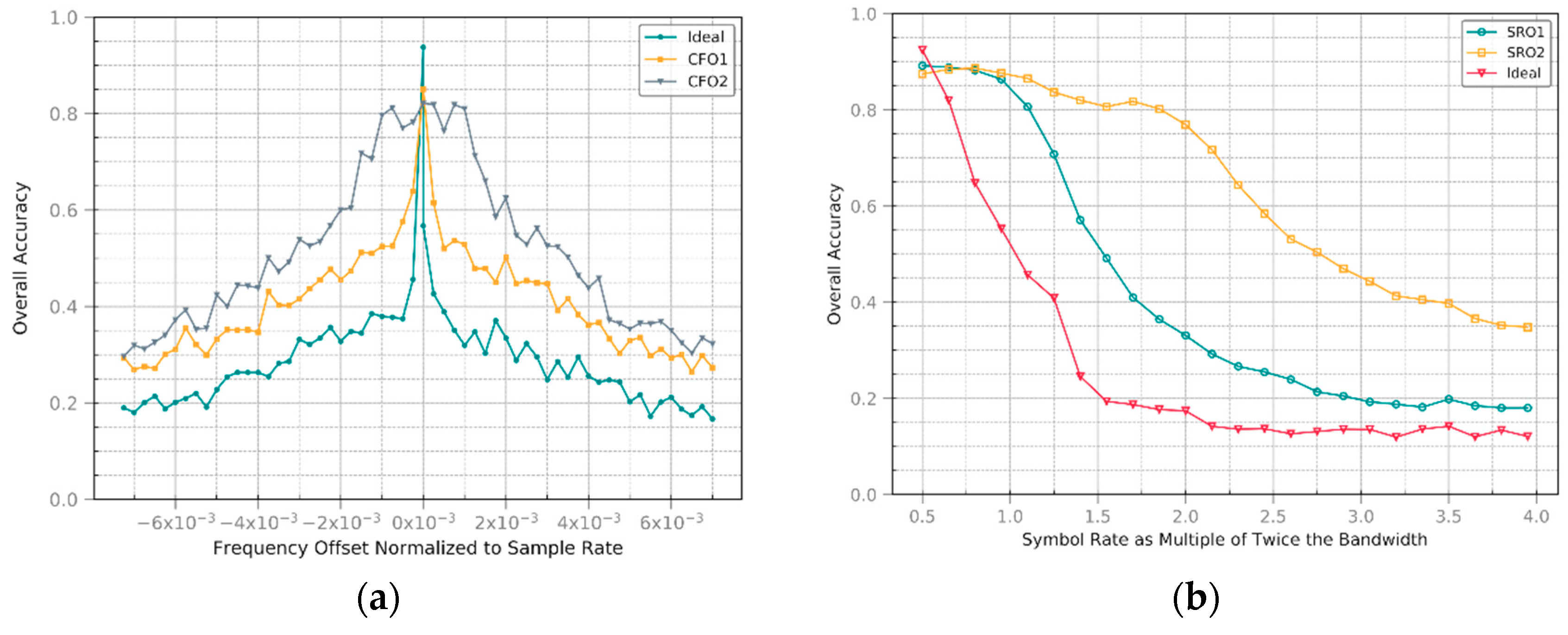
19] discussed the impact of deep neural network design on communication receivers. Besides, the effects of certain errors bound in detection and isolation are analyzed. It was shown that for the frequency offset and sample rate offset not covered in the training samples, there is a significant decline in the test samples. Summarizing the existing research on the application of classification on raw baseband signals, there is less consideration of the errors introduced in signal detection and isolation and the robustness of the algorithm performance in such offsets. However, in blind wide-band signal processing, these offsets caused by parameter estimation or hardware defects are difficult to avoid. In the AMR system, a technique that can reduce the influence of signal isolation and detection error needs to be proposed. In this article, we study the AMR method based on the raw IQ signals under parameter estimation errors. Firstly, the influence of parameter estimation errors on the performance of the CNN classifier is analyzed. Then, an AMR method based on a spatial transform network (STN) is proposed. By applying this improved model, the robustness of the AMR method under parameter estimation errors has been significantly improved.
The remainder of this paper is presented as follows: In Section 2, we provide an overview of flow for blind wideband signal capture model. Section 3 introduces the classification method based on STN. Section 4 introduces the evaluation setup for AMR. Section 4 presents simulations and results. Finally, Section 5 concludes the paper.

2. Wireless Signal Modulation Recognition Model

In digital communications in real radio frequency (RF) environments, the transmitter forms a binary bit stream of information. After that, the bits stream is encoded and modulated, and finally transmitted via the wireless channel. During the modulation process, the baseband signal is moved to the shifted by the carrier frequency to produce the wireless signal.
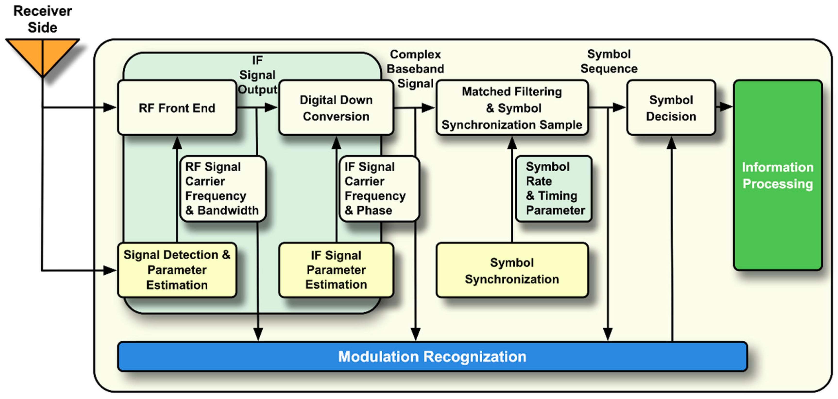
A typical flow of modulation recognition signal processing is presented in Figure 1. At the receiving end, we consider a typical communication receiver in the noncooperative mode. In general, there is only a partial or even minimal prior knowledge of communication. The receiver monitors the activity of the radio frequency (RF) signal in the electromagnetic spectrum of interest through a spectrum analyzer and gives an estimated value of the centre frequency, the bandwidth of the signal. Based on these parameters, the receiver through the bandpass filtering and downconverts to flit the signal capture to appropriate intermediate frequency (IF). For the digital communication signal, the phase-locked loop is used to further accurately extract the carrier frequency and phase parameters of the intermediate frequency signal. Then, using the orthogonal downconversion technique, the baseband signal of the unknown modulation mode is outputted at the output end of the matched filter. Then, parameters such as baud rate and symbol timing are obtained by symbol synchronization technology, matched filtering, and synchronous sampling are performed to obtain a symbol sequence of an unknown modulation mode. The signal is then subjected to subsequent demodulation. Our approach focuses on AMR on complex baseband signals, which is a coherent, asynchronous AMR method. During signal reception and processing, due to imperfections in the detection and isolation stages, carrier frequency estimation errors, bandwidth estimation errors, etc. are introduced during the RF signal to the IF signal acquisition process. In the processing of the intermediate frequency signal to the complex baseband signal, carrier frequency and phase synchronization errors are also introduced. Then, given the channel impairments and hardware defects of the receiver, the baseband signal we obtained is the corrupted version of the originally transmitted signal. In the AMR application for the original baseband signal, the definition and evaluation of these impairments is very important. We define typical signal impairments:
  • Frequency Offset: Frequency offset is introduced during the RF signal isolation phase and IF signal parameter estimation. The receiver local oscillator (LO) introduces frequency deviation due to hardware impairments.
  • Phase offset: Phase offset is caused by the frequency offset of LO, which causes an instantaneous phase drift of signal captures.
  • Timing drift: Timing drift is caused by unmatched sampling rates. It is introduced due to the estimated bandwidth deviation of the RF signal isolation phase. Besides, the sampling rate error is introduced due to hardware impairment of the receiver LO.
  • Noise: Noise introduced by components such as the antennas and receivers. We usually model this noise as additive white Gaussian noise (AWGN).
Signal capture and processing flow of the receiver includes: amplifying, mixing, low-pass filtering, and analog-to-digital conversion. Then, the raw baseband IQ signal is obtained. N-th point sampling are performed on the baseband IQ signal. We present the values as r r a w N . This matrix is the input sequence of the AMR, which contains information if signal captures such as the type of wireless technology, the type of modulation method, interferer, etc. The task of AMR is to obtain the type of modulation through this segment of the signal capture. Therefore, the output of the end-to-end system can be expressed as l . The output of the system output is the judgment of AMR, which is the highest confidence of modulation type in the result set. Then, the observed data consists of k pairs of input and output. For AMR tasks, these pairs can be organized into datasets S , which can be denoted as:
S = { ( r r a w 1 ,   l 1 ) , ( r r a w 2 ,   l 2 ) , ( r r a w k ,   l k ) }

3. Proposed Method

To effectively perform the raw complex baseband signal AMR, we further clarify the four typical errors defined in Section 2. This definition helps us to generate simulation offsets and propose corresponding methods for generating mechanisms. Among these four kinds of errors defined in Section 2, the frequency offset and phase offset are caused by frequency offset, and the time drift is caused by the sample rate. Therefore, the method we propose mainly focuses on frequency offset, sample rate offset and noise. Our basic idea is to adaptively correct the above offset by designing a parameters transformer module. We introduce the attention model in the field of computer vision into AMR to solve this problem.
Spatial transformer networks (STN) [20] is the deep learning attention model proposed in 2015. It is an end to end feedforward network. The basic structure of STN includes localization net, grid generator, and sampler. The localization net provides parameter regression, the grid generator implements pixel coordinates, and the sampler implements microscopic coordinate transformation. In the field of computer vision, STN is widely used to implement image translation, scaling, rotation etc. through 2D affine transformation [21], superior performance in image alignment tasks is shown in the paper. In the geometric corrections of image synthesis, STN also has good results [22], robust normalization is performed by application of the 3D morphable model. O’shea [23] made an initial attempt to introduce STN into the field of radio signals. He designed an attention model based on CNN. The classification accuracy test was carried out on the RadioML 2016.04C [24] dataset, but the results did not reflect the role of the proposed method in signal synchronization and regularization representation.
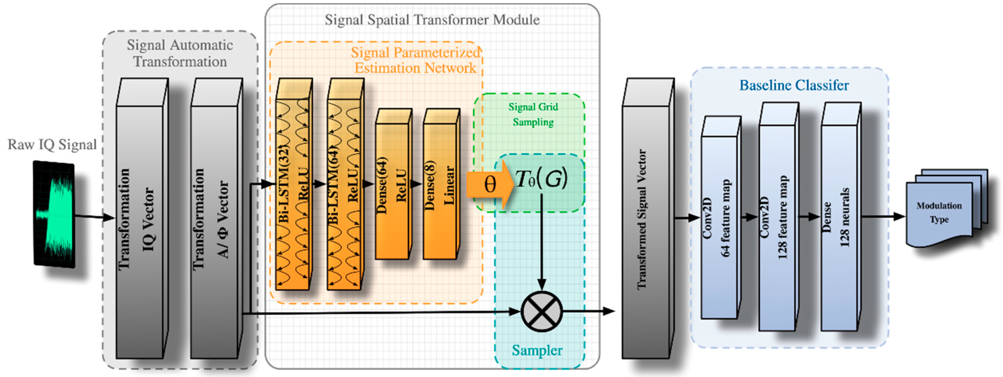
We propose a new signal classification network based on STN architecture, which introduces the parameter transformation of the radio domain. This architecture normalizes the signal before classification, automatically reducing the impact of sample rate offset and frequency offset on classification. Through the introduction of this attention model, our classification results exceed our nonattention model, the classifier discriminant task is reduced, and the network performance is improved. The framework we propose consists of two parts, one is the signal classifier and the other one is signal spatial transformer module (SSTM). The proposed AMR system is shown in Figure 2. To establish an AMR system under the parameter estimation error. We must develop a transform that adaptively corrects the estimation errors described above. Therefore, we designed the STN-based signal spatial transformer module (SSTM). This module is cascaded before the signal classifier. SSTM includes automatic transformation and the signal parameter estimation network, grid generator, and signal sampler. After SSTM, we implement a CNN network for signal classification. We evaluated various network structures with variation between activation functions, connections, and loss function. The structure and hyperparameters of the network have been experimentally adjusted to optimize performance, and detailed parameter setting is listed in Section 4. We regard this CNN classifier as the baseline for AMR. We design the structure of the proposed method through a lot of experiment. An important principle is to design the SSTM separately after using the optimal baseline classifier as the evaluation criteria. In this section, we mainly introduce the implementation of SSTM.

3.1. Automatic Signal Transformation

In this paper, automatic signal transformation involves two signal processing methods, one is the real-value equivalent representation of the raw complex baseband signal, and the other is based on the original signal amplitude and phase extraction representation. These two transformations are based on signal modulation characteristics. We apply these two transformations to the raw baseband signal r r a w N for better extraction of features. The transformations are as follows:
Transformation (IQ vector): the k-th point raw signal data r r a w N can be translated to the k-th feature vector x k N . Then, the in-phase and quadrature component parts of the complex baseband signal r r a w N are represented as two real-valued matrices x I , x Q , that is:
x k I Q = [ x I T x Q T ] T
For x k I Q 2 × N , mathematically, the transformation can be written as
f T r a n 1 : N N × 2 r r a w     x k I Q  
Transformation ( A   /   ϕ vector): the k point raw signal data r r a w is mapped into the k-th feature vector x k I Q . We use the phase vector x A and magnitude vector x ϕ to represents x k I Q , that is:
x k A / ϕ = [ x A T x ϕ T ] T
where, the x A and x ϕ is calculated with
x ϕ ( n ) = ( x I ( n ) ) x A ( n ) = arctan 2 ( x I ( n ) x Q ( n ) ) ,   n = 0 , 1 , , N 1
In this transformation, we use the atan2 function to obtain continuous phase changes. The ordinary atan function causes the sign of the phase to change, losing the phase information of the second and third quadrants. Then, a real-valued convolution layer is used to augment the feature map. For x k A / ϕ , we use M convolution kernels with 2 × 8 receptive fields to convolve and get the transformed output as
f T r a n 2 : N × 2 N × 2 N × M × 2 x k I Q   x k A / ϕ     x k T r a n 2

3.2. Signal Parameterized Estimation Network

The signal parameterized estimation network takes the input feature map U M × N × 2 , outputs a set of signal estimation parameters θ . θ is a set of parameters used for signal transformation. In this paper, we consider the variation caused by time drift, symbol rate conversion, sample rate offset, and centre frequency offset. Time drift involves shifting the signal with the correct initial amount. The symbol rate conversion and sample rate offset can be corrected using the correct sample increment resampling and interpolation. We implement these two changes to approximate the 2D affine transformation in the image.
( θ 11 θ 12 θ 13 θ 21 θ 22 θ 23 )
For centre frequency offset correction, we estimate the phase offset for each sample point to compensate with
n θ 3 ,   n = 0 , 1 , , N 1
The phase noise caused by the CFO is compensated by the phase offset of a constant term θ 4 .
θ = f e s t ( U ) is used to represent the signal parameterized estimation function. Within the scope of this paper, θ has eight parameters, including six parameters of the 2D affine transformation and two parameters of phase and carrier frequency recovery.
We use a deep neural network model to implement θ . Long short-term memory (LSTM) [25] network is a recurrent neural network suitable for processing and predicting important events with relatively long intervals and delays in time series. LSTM is an effective technique for solving long-order dependency problems. Because of the specificity of radio data, the sampling points are highly in temporal correlation. Different modulation signals have trip points in phase and amplitude. The range of signal contextual information is large, and this problem causes the influence of the input of the hidden layer on the network output to decline as the network loop continues to recurse. Therefore, we use Bi-directional LSTM [26] to extract radio signal modulation features, which is an extended model of LSTM. The Bi-LSTM contains two input sequences, one is the positive sequence and the other is the inverted sample of the input sequence. The two-way cyclic network structure can perform well on sequence classification problems. The architecture of Bi-LSTM presents in Figure 3.
In the signal parameterized estimation network model, we implemented two Bi-LSTMs, then two fully connected layers. Finally, θ is obtained by the linear activation function. We use the appropriate weight initialization, dropout, and regularization tricks to achieve optimal performance under this network model.

3.3. Signal Grid Sampling

We normalize signal by transformation models, which are widely used in CV. The transformation model is capable of fitting geometric distortions between the source image and the background image by geometric transformation. The transformation models that can be used are as follows: rigid transformation, affine transformation, perspective transformation, and non-linear transformation. To perform the deformation of the input feature map, we apply resampling and transformation by sample point T ( θ ) . In our method, the resampled pixels ( x i t , y i t ) form the output feature map V M × N × 2 . Based on the analysis of the radio signal characteristics in the previous part, we consider the variation caused by time drift, symbol rate conversion, sample rate offset, and centre frequency offset. Time drift involves shifting the signal with the correct initial amount. This task is similar to translation in the 1D affine transformation. Translation in the time dimension provides correction for time drift. The symbol rate conversion and sample rate offset can be corrected using the correct sample increment resampling and interpolation. This task is similar to scaling in the 2D affine transform. We implement these two changes to approximate the 2D affine transformation in the image. We define the transformation T ( θ ) , consisting of two parts. One is the 2D affine transform A θ , then there is the frequency and phase compensations R θ . In this affine case, the pointwise transformation is
( x i s y i s ) = A θ R θ ( x i t y i t 1 ) = ( θ 11 θ 12 θ 13 θ 21 θ 22 θ 23 ) ( n θ 3 + θ 4 ) ( x i t y i t 1 ) ,   i = 0 , 1 , , M × N 1 n = c e i l ( i / M )  
where ( x i s , y i s ) are the target coordinates of the grid in the output feature map. The resampling application applies the parameters we estimated by signal parameterized to the signal transformation.

4. Evaluation Setup

To mitigate the impact of estimation errors in the detection and isolation stage of a receiver on AMR, we introduce the attention model of the computer field to AMR. Synthetic radio datasets containing different estimation errors are used to verify the validity of our proposed method.

4.1. Dataset Description

To evaluate the classification performance of our proposed method, we use datasets that simulate the centre frequency offset and sample rate offset to train and test the method. In addition to the two major errors in the datasets, we also consider the damage in a variety of signal transmissions, including signal arrival times, nonimpulsive delay spread, Doppler offsets, and Gaussian thermal noise. Since these common time-varying random channel effects exist in most wireless systems, we include these effects in the datasets as much as possible.
The dataset includes eight digital modulation methods, namely CPFSK, 4-PAM, GFSK, BPSK, QPSK, 8-PSK, 16-QAM, and 64-QAM. We extract the baseband signal of 128 sample points in the signal stream generated by the combination of each modulation mode, estimation error, and channel impairment. We divide signal captures into IQ two-way storage as with the signal representation described above. With each frequency offset, sample rate offset, and SNR combination, we get 500 test signal captures and 500 training signal captures. Each sample includes 3–20 symbols. The signal captures are generated at various SNRs between −10 and 20 dB. To simulate different degrees of frequency offset and sample rate offset, we use the datasets listed in Table 1, ideal detectors without frequency and sample rate offsets (ideal), Dataset with various sample rate offsets (SRO 1 and SRO 2), detector with varying carrier frequency offset (CFO 1 and CFO 2). It is worth noting that the datasets listed in Table 1 are training sets. We train on training sets with different frequency and sample rate offsets to evaluate the models’ tolerance to parameters estimation error.

4.2. Implement Details

We use Keras [27] and Tensorflow [28] mixed programming. Keras is used for definitions of standard layers, such as pooling, convolution, dense, and Softmax. Tensorflow is mixed with defining custom layers in SSTM. We use a deep learning workstation with the high-performance central processing unit (CPU) and NVIDIA 1080Ti graphics card. The neural networks parameters are optimized by the ADAM [29] algorithm. We train 500 epochs on the networks with an optimized learning rate. The learning rate is estimated based on Bayesian optimization [30] with the open source Hyperopt [31] library. Hyperparameters used for training are listed in Table 2. The structure of the baseline network is shown in Table 3.

5. Simulations

To mitigate the impact of estimation errors in the detection and isolation stage of a receiver on AMR, we introduce the attention model of the computer field to AMR. Synthetic radio datasets containing different estimation errors are used to verify the validity of our proposed method.

5.1. Baseline Convolution Networks

To evaluate the impact of CFO on classification performance, we use CNN as a baseline. The baseline network uses training and optimizing methods described in [16], which can representatively evaluate classification performance under different degrees of offset. We train the baseline networks on the CFO1 and CFO2 datasets. For test scenarios, the CFO is shifted from −6% to 6% of the sample rate. Figure 4 shows the classification accuracy in the CFO1 and CFO2 scenarios.
For frequency offset outside the training range, the classification performance of CNN classifiers declines rapidly. The consistent decline in performance occurred in both training datasets. This shows that the baseline classifier is sensitive to frequency offsets. Besides, at all frequency offsets, as the SNR is shifted from −10 to 10 dB, the classification accuracy continues to increase significantly. However, when SNR exceeds 10 dB, the classification accuracy cannot be further improved. We believe this is because as the SNR increases, higher SNR does not provide more useful information to help optimize network parameters.
We test on signal captures with sample rate range from 1 to 8 multiples of the bandwidth to verify the effect of sample rate offset on modulation recognition performance. We train the baseline networks on the SRO1 and SRO2 datasets. As presented in Figure 5, for sample rate offsets outside the training range, the classification accuracy decreases rapidly, and this reduction occurs in both test set scenarios. Besides, this reduction in classification performance shows consistency across all SNR scenarios. At the same sample rate offset, the classification accuracy versus SNR is similar to frequency offset scenario.
In Figure 6, we present a sectional view of overall accuracy versus the frequency offset and sample rate when SNR is fixed at 20 dB. These simulations help to show the trends observed in Figure 4 and Figure 5. Numerical analysis for all training scenarios in typical SNRs and offsets is shown in Table 4. In all offsets and training set scenarios, as the SNR increase, the classification performance can be significantly improved. For low frequency and sample rate offsets, the classifiers on all training sets have similar performance. For medium frequency and sample rate offsets, the classifiers obtained on the SRO2 and CFO2 training sets perform significantly better than the classifiers obtained on the SRO1 and CFO1 training sets. As frequency and sample rate offsets increase, the classification performance decreases consistently across all SNR and training set scenarios.

5.2. Convolution Networks with SSTM

We apply the module proposed in Section 2 to the baseline CNN network. Using the same training and test scenarios as the baseline, we get typical results shown in Figure 7 for the CFO1 and SRO1 datasets. In Figure 7a, it is shown that our method achieves a classification accuracy improvement of 5% to 30% over the absolute value of the frequency offset from 0.1% to 0.4%. For smaller frequency offsets, the classification performance is improved more. The proposed method achieves a broader performance gain over a larger range of training offsets. The increase in classification accuracy arises within the entire test dataset. For the performance decline caused by sample rate offset, our method shows better results. In Figure 7b, the optimization of classification performance is demonstrated in two aspects: Firstly, due to the introduction of SSTM, higher classification accuracy is obtained in the sample rate within the range of training datasets. Then, a consistent classification accuracy improvement is produced at sample rates outside the range of the training dataset. When the test sample rate range exceeds the training dataset, the classification accuracy of our method will not drop drastically.
In Figure 8, we plot a cross-sectional view of overall accuracy versus frequency offset or symbol rate at a fixed 20 dB SNR. According to the different processing steps of the received signals, the signal models can be divided into the following three types: model of radio frequency signals (MRF), model of baseband signals (MBB), and model of the output of the matched filter at receiver (MMF). According to the preprocessing requirement, the AMR method can be divided into three types: environment of ideal synchronization (EIS) algorithm, environment of nonideal synchronization (ENIS) algorithm, and environment of no synchronization (ENS) algorithm. Our method is an ENS method under the MBB signal model. Therefore, we compare our method with the DL-based method of different synchronization requirements under MBB model. For ENS and ENIS methods, we compare the methods with RTN, which is proposed by O’shea [23]. For EIS methods, we compare with the CNN method with the best performance in the DL-based method, namely the baseline method in this article. Besides, the effects of different signal parameterized estimation network structures on classification performance are evaluated, including multilayer perceptrons and CNN. We represent these frameworks as SSTM_Dense and SSTM_CNN. The compared networks have undergone the same optimal hyperparametric search to achieve optimal performance.
It is shown in Figure 8a that, for the frequency offset, the methods based on our network model provide a certain performance improvement. The Bi-LSTM method provides the best results, followed by CNN and multilayer perceptrons [32]. It is shown in Figure 8b that for the symbol rate, Bi-LSTM in our network model yields an increase in accuracy overall test ranges. The network performance improvement with the addition of the CNN-based SSTM module is gradual, with performance decline at higher dynamic range symbol rates. We believe this is because CNN’s limited spatial convertibility is unable to cope with a wide range of difference in signal captures, resulting in the inability to effectively train at larger symbol rates. The multilayer perceptron is close to the baseline performance. Overall classification accuracies of all methods at typical offsets are shown in Table 5, with SNR fixed at 20 dB. With all methods increasing with frequency or sampling rate offset, the classification accuracy is significantly reduced. The proposed method achieves optimal performance with frequency and sample rate shifts. Our method has a promotion of 51% at high sampling rate offset, which indicates that the application of SSTM corrected sample rate offset implicitly. Thereby, the signals of various sample rate offset are normalized. This processing reduces the classifying difficulty of the baseline classifier.

6. Conclusions

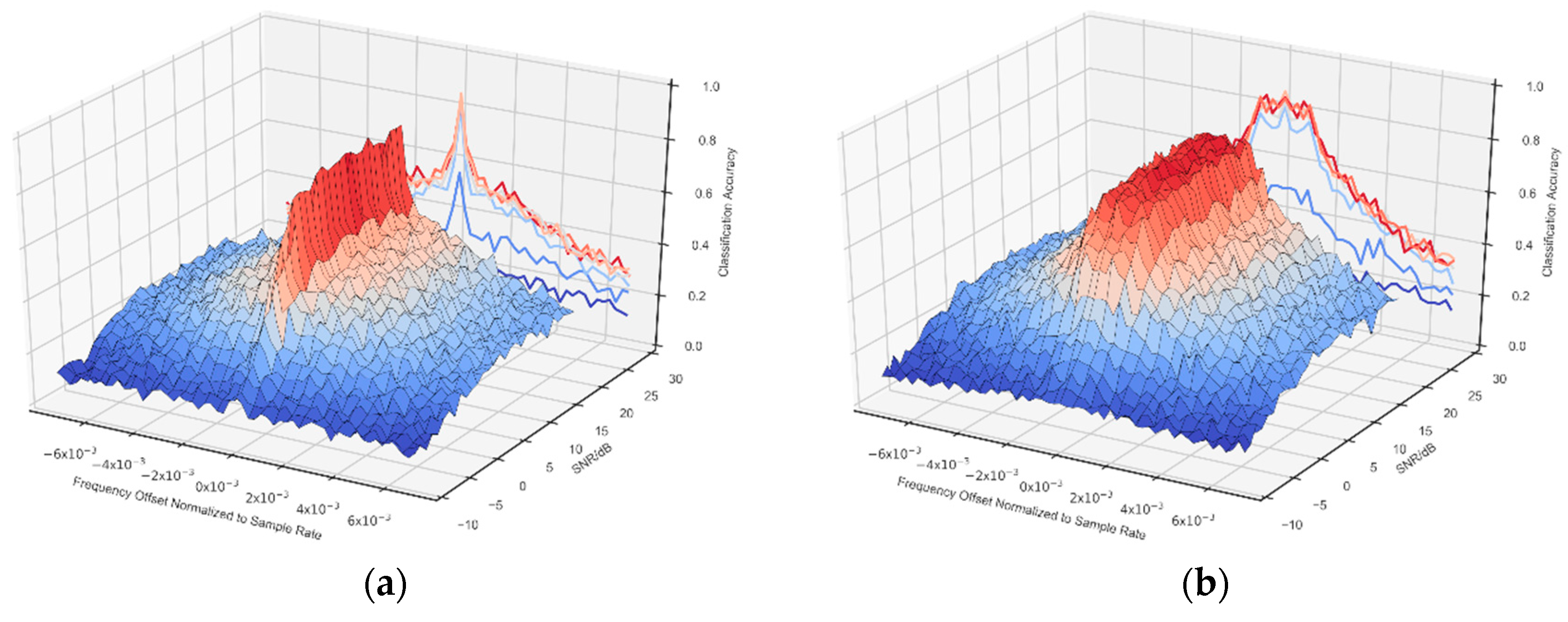
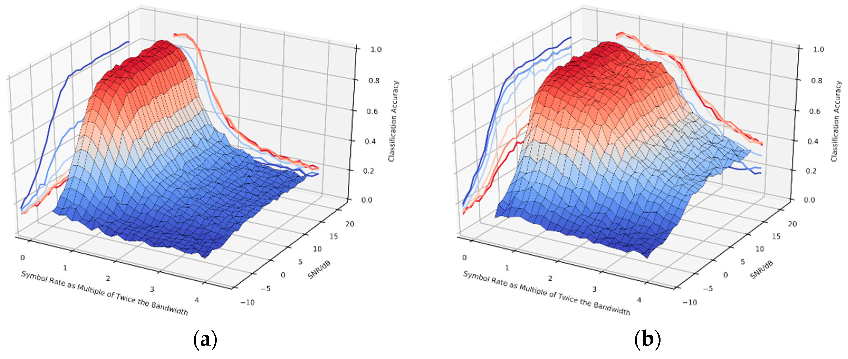
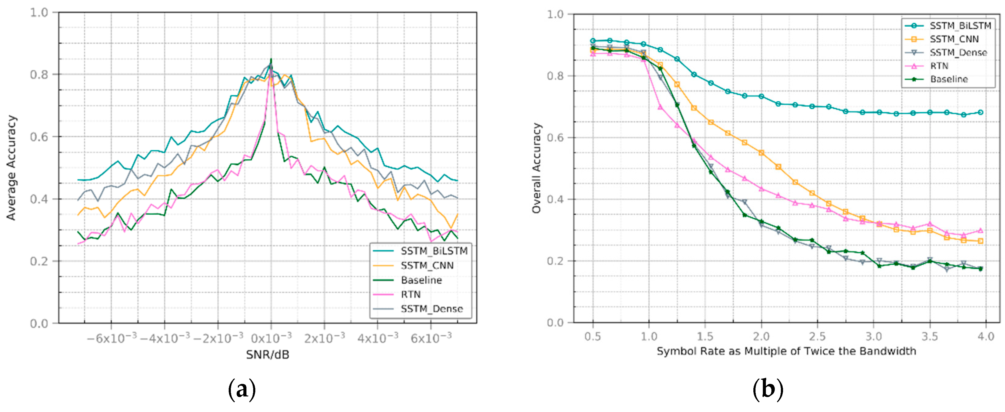
Using deep neural networks for AMR directly on IQ signals is currently common. However, the performance of the network in the actual scene is greatly affected by errors introduced in the signal acquisition process. Also, automatic modulation recognition for different symbol rate signals is also an urgent problem to be solved without considering resampling. Aiming at the dependence of modulation identification on parameter estimation error, such as carrier frequency and symbol rate, we proposed an integrated method of parameter estimation and modulation recognition based on the attention model. We establish a baseline CNN network to evaluate the effect of parameter estimation errors introduced during detection and isolation. With the idea of a spatial transformation network in the field of deep learning, we concatenate the SSTM before convolutional neural networks. The signal transformation network eliminates signal variations introduced in the wireless channel and receiver hardware by adaptively applying parameter transformations. This includes resampling to adjust the time offset, symbol rate, and clock recovery, mixing with the carrier to correct frequency offset. Applying this improved model to AMR significantly reduces the dependence of recognition performance on parameter estimation. The results prove that our method can bring significant performance improvement under the influence of offset. Our method realizes the integration of parameter estimation and signal captures classification, reduces the dependence on parameter estimation errors, and performs well under fading channel. However, our method exhibits greater tolerance to the offsets in symbol rate estimation than frequency offset, and this result deserves further study. Besides, no further analysis is performed on the SSTM processed signals, which require further research.
In future work, we plan to explore the application of the attention model in AMR, such as channel blind equalization, synchronization, and resampling.

Author Contributions

All authors read and approved the manuscript. Conceptualization, M.L. and G.L.; Methodology, M.L.; Software, M.L.; Validation, C.Z.; Formal Analysis, M.L.; Investigation, O.L.; Resources, O.L.; Data Curation, G.L.; Writing-Original Draft Preparation, M.L.; Writing-Review & Editing, G.L.; Visualization, C.Z.; Supervision, O.L.; Project Administration, G.L.; Funding Acquisition, O.L.

Funding

This research was funded by [the National Natural Science Foundation of China] grant number [61501517].

Conflicts of Interest

The authors declare no conflict of interest.

References

  1. Dobre, O.A.; Abdi, A.; Bar-Ness, Y.; Su, W. Survey of automatic modulation classification techniques: Classical approaches and new trends. Commun. IET 2007, 1, 137–156. [Google Scholar] [CrossRef]
  2. Miao, S.; Bar-Ness, Y.; Wei, S. Blind OFDM Systems Parameters Estimation for Software Defined Radio. In Proceedings of the IEEE International Symposium on New Frontiers in Dynamic Spectrum Access Networks, Dublin, Ireland, 17–20 April 2007. [Google Scholar]
  3. Dobre, O.A.; Abdi, A.; Bar-Ness, Y.; Su, W. Blind Modulation Classification: A Concept Whose Time Has Come. In Proceedings of the IEEE/SARNOFF Symposium on Advances in Wired & Wireless Communication, Princeton, NJ, USA, 18–19 April 2005. [Google Scholar]
  4. Wu, H.C.; Saquib, M.; Yun, Z. Novel automatic modulation classification using cumulant features for communications via multipath channels. IEEE Trans. Wirel. Commun. 2008, 7, 3098–3105. [Google Scholar]
  5. Fucai, Z.; Yihua, H.; Shiqi, H. Classification using wavelet packet decomposition and support vector machine for digital modulations. J. Syst. Eng. Electron. 2008, 19, 914–918. [Google Scholar] [CrossRef]
  6. Dobre, O.A.; Oner, M.; Rajan, S.; Inkol, R. Cyclostationarity-based robust algorithms for QAM signal identification. IEEE Commun. Lett. 2012, 16, 12–15. [Google Scholar] [CrossRef]
  7. Haykin, S. Cognitive radio: Brain-empowered wireless communications. IEEE J. Sel. Areas Commun. 2005, 23, 201–220. [Google Scholar] [CrossRef]
  8. Mitola, J.; Maguire, G.Q. Cognitive radio: Making software radios more personal. IEEE Pers. Commun. 1999, 6, 13–18. [Google Scholar] [CrossRef]
  9. Axell, E.; Leus, G.; Larsson, E.G.; Poor, H.V. Spectrum sensing for cognitive radio: State-of-the-art and recent advances. IEEE Signal Process. Mag. 2012, 29, 101–116. [Google Scholar] [CrossRef]
  10. Shimaoka, S.; Stenetorp, P.; Inui, K.; Riedel, S. Neural architectures for fine-grained entity type classification. arXiv, 2016; arXiv:1606.01341. [Google Scholar]
  11. Krizhevsky, A.; Sutskever, I.; Hinton, G.E. ImageNet Classification with Deep Convolutional Neural Networks. In Proceedings of the International Conference on Neural Information Processing Systems (NIPS), Lake Tahoe, NV, USA, 3–6 December 2012; pp. 1097–1105. [Google Scholar]
  12. Yu, D.; Deng, L. Automatic Speech Recognition: A Deep Learning Approach; Springer: Berlin, Germany, 2014. [Google Scholar]
  13. Pławiak, P.; Rzecki, K. Approximation of Phenol concentration using computational intelligence methods based on signals from the metal-oxide sensor array. IEEE Sens. J. 2015, 15, 1770–1783. [Google Scholar]
  14. Yıldırım, Ö.; Pławiak, P.; Tan, R.-S.; Acharya, U.R. Arrhythmia detection using deep convolutional neural network with long duration ECG signals. Comput. Biol. Med. 2018, 102, 411–420. [Google Scholar] [CrossRef] [PubMed]
  15. Shi, C.-T. Signal pattern recognition based on fractal features and machine learning. Appl. Sci. 2018, 8, 1327. [Google Scholar] [CrossRef]
  16. O’Shea, T.J.; Hoydis, J. An introduction to deep learning for the physical layer. IEEE Trans. Cogn. Commum. Netw. 2017, 3, 563–575. [Google Scholar] [CrossRef]
  17. O’Shea, T.J.; Roy, T.; Clancy, T.C. Over-the-air deep learning based radio signal classification. IEEE J. Sel. Top. Signal Process. 2018, 12, 168–179. [Google Scholar] [CrossRef]
  18. O’Shea, T.J.; Corgan, J.; Clancy, T.C. Convolutional Radio Modulation Recognition Networks. In Proceedings of the International Conference on Engineering Applications of Neural Networks, Aberdeen, UK, 2–5 September 2016; pp. 213–226. [Google Scholar]
  19. Hauser, S.C.; Headley, W.C.; Michaels, A.J. Signal Detection Effects on Deep Neural Networks Utilizing Raw IQ for Modulation Classification. In Proceedings of the IEEE Military Communications Conference (MILCOM), Baltimore, MD, USA, 23–25 October 2017; pp. 121–127. [Google Scholar]
  20. Jaderberg, M.; Simonyan, K.; Zisserman, A. Spatial Transformer Networks. In Proceedings of the Neural Information Processing Systems (NIPS), Montreal, QC, Canada, 7–12 December 2014. [Google Scholar]
  21. Chen-Hsuan, L.; Simon, L. Inverse Compositional Spatial Transformer Networks. In Proceedings of the IEEE Conference on Computer Vision and Pattern Recognition (CVPR), Honolulu, HI, USA, 21–26 July 2017. [Google Scholar]
  22. Anil, B.; Patrik, H.; William, A.S. 3D Morphable Models as Spatial Transformer Networks. In Proceedings of the IEEE Conference on Computer Vision Workshop (ICCV), Venice, Italy, 22–29 October 2017. [Google Scholar]
  23. O’Shea, T.J.; Pemula, L.; Batra, D.; Clancy, T.C. Radio Transformer Networks: Attention Models for Learning to Synchronize in Wireless Systems. In Proceedings of the Asilomar Conference on Signals, Systems & Computers (ACSSC), Pacific Grove, CA, USA, 6–9 November 2016. [Google Scholar]
  24. O’Shea, T.J.; West, N. Radio Machine Learning Dataset Generation with GNU Radio. In Proceedings of the 6th GNU Radio Conference, Boulder, CO, USA, 6 September 2016. [Google Scholar]
  25. Gers, F.A.; Schmidhuber, J.; Cummins, F. Learning to forget: Continual prediction with LSTM. Neural Comput. 2000, 12, 2451–2471. [Google Scholar] [CrossRef] [PubMed]
  26. Shabanian, S.; Arpit, D.; Trischler, A.; Bengio, Y. Variational Bi-LSTMs. arXiv, 2017; arXiv:1711.05717. [Google Scholar]
  27. Chollet, F. Keras. Available online: https://github.com/fchollet/keras (accessed on 24 November 2015).
  28. Abadi, M.A.A. Tensorflow: Large-Scale Machine Learning on Heterogeneous Systems, Software. Available online: http://tensorflow.org/ (accessed on 4 June 2015).
  29. Kingma, D.P.; Ba, J. Adam: A Method for Stochastic Optimization. In Proceedings of the International Conference on Learning Representations (ICLR), Banff, AB, Canada, 14–16 April 2014. [Google Scholar]
  30. Pelikan, M. Bayesian Optimization Algorithm. In Hierarchical Bayesian Optimization Algorithm; Springer: Berlin/Heidelberg, Germany, 2005; pp. 31–48. [Google Scholar]
  31. Bergstra, J.S.; Yamins, D.; Cox, D.D. Hyperopt: A Python Library for Optimizing the Hyperparameters of Machine Learning Algorithms. Available online: http://hyperopt.github.io/ (accessed on 23 May 2015).
  32. Bishop, C.M. Neural Networks for Pattern Recognition; Oxford University Press: New York, NY, USA, 1995. [Google Scholar]
Figure 1. Recognition Signal Processing Flow.
Applsci 09 01010 g001
Figure 2. The framework of the proposed method with SSTM for directly using raw in-phase and quadrature (IQ) samples.
Applsci 09 01010 g002
Figure 3. The bi-directional long short-term memory (Bi-LSTM) structure in the signal parameterized estimation network.
Applsci 09 01010 g003
Figure 4. Overall classification accuracy of baseline classifier for various training scenarios vs. frequency offset and SNR. (a) CFO1; (b) CFO2.
Applsci 09 01010 g004
Figure 5. Overall classification accuracy of baseline classifier for various training scenarios vs. sample rate offsets and SNR. (a) SRO1; (b) SRO2.
Applsci 09 01010 g005
Figure 6. Overall classification accuracy for various offsets in Ideal, SRO1, SRO2, CFO1, CFO2, with SNR fixed at 20 dB (a) frequency offsets in Ideal, CFO1, CFO2; (b) sample rate offsets in Ideal, SRO1, SRO2.
Applsci 09 01010 g006
Figure 7. Overall classification accuracy of the classifier with SSTM for various training scenarios vs. frequency offset and SNR. (a) CFO1; (b) SRO1.
Applsci 09 01010 g007
Figure 8. Overall classification accuracy with various offsets in SRO1 and CFO1 scenarios with the aforementioned methods. (a) CFO1; (b) SRO1.
Applsci 09 01010 g008
Table 1. Considered neural network training scenarios.
Dataset NameFrequency Offset RangeSample Rate Range (Multiple of Bandwidth)
IdealNo offset2
CFO 10.05% of sample rate2
CFO 20.1% of sample rate2
SRO 1No offset1–1.5
SRO 2No offset1–4
Table 2. Hyperparameters in signal spatial transformer module (SSTM)-based method training.
HyperparametersValue
Loss FunctionCategorical Crossentropy
OptimizerADAM
Dropout Rate0.4
InitializerLecun Normal [18]
Learning Rate0.0024 (baseline), 0.00081(SSTM)
Batch Size256
Epochs500
Table 3. Structure of baseline classifier.
Layer TypeInput SizeParametersActivation Function
Convolution Layer128 × 1286 × 6 filter kerne
l64 feature maps
Leaky ReLU
Pooling Layer128 × 128 × 642 × 2 max poolingNone
Convolution Layer64 × 64 × 643 × 3 filter kernel
32 feature maps
Leaky ReLU
Pooling Layer64 × 64 × 322 × 2 max poolingNone
Flatten32 × 32 × 32Flatten feature mapNone
Dense32,76864 neuronsReLU
Dense648 neuronsSoftmax
Table 4. Performance comparison for different training scenarios in typical SNR.
ScenariosSNRLow OffsetMedium OffsetHigh Offset
SRO1High0.890.290.18
Medium0.800.240.17
Low0.250.180.15
SRO2High0.880.710.34
Medium0.800.620.31
Low0.320.270.17
CFO1High0.850.410.31
Medium0.790.390.28
Low0.520.250.17
CFO2High0.820.530.37
Medium0.780.480.30
Low0.470.280.20
Table 5. Performance comparison for methods versus typical offsets in SRO1 and CFO1 scenarios.
FrameworkOffsetSRO1CFO1
BaselineHigh0.170.31
Medium0.700.41
Low0.880.85
RTNHigh0.290.31
Medium0.640.44
Low0.870.83
SSTM_CNNHigh0.260.35
Medium0.770.53
Low0.880.80
SSTM_DenseHigh0.170.44
Medium0.700.57
Low0.890.83
SSTM_BiLSTMHigh0.680.46
Medium0.850.62
Low0.910.84

