A Novel Method to Assess Safety of Buried Pressure Pipelines under Non-Random Process Seismic Excitation based on Cloud Model

Abstract

It is necessary to conduct a safety assessment for pipelines which are regarded as important lifeline projects after an earthquake. Since the random process of loading in earthquake engineering requires a large amount of samples, this paper establishes a non-random vibration method based on convex model theory and applies it to small sample engineering. Moreover, a space–time analytical model of buried pipeline and a finite element model are established to solve the dynamic response of pipelines with non-random process seismic excitation. Furthermore, the randomness of the stress values of the pipeline subjected to earthquake and the fuzziness of the degree of damage to pipelines are considered. Therefore, a novel method for assessing damage to pipelines is proposed based on cloud model. The results indicate that an analysis of non-random vibration combined with the cloud inference method can solve the fuzziness and randomness of the quantitative description and qualitative concept conversion for damage evaluation of pipelines. The method is also an adaptive and effective assessment method for pipelines exposed to earthquake and is able to promote safety management of pipeline engineering.

1. Introduction

Recently, pipelines have become regarded as important lifeline projects for transporting energy [1,2]. As the dependence of global energy demand on oil/gas grows steadily, pipelines have become the primary transportation infrastructure [3]. Many methods for monitoring the condition of pipelines and for leak detection/pinpointing through proper sensors have been developed [4,5,6,7]. However, the 21st century is an era of frequent earthquakes [8,9]. The Hyogo-Ken Nanbu earthquake of 1995 in Japan was a recent example of an earthquake which caused damage to pipelines; it not only led to gas leakage, but also caused fires [10]. Furthermore, the Chi-Chi earthquake of 1999 in Taiwan caused serious damage to pipelines along with serious economic losses and environmental damage [11].

In order to analyze the response of pipelines to seismic loads, numerous research methods have been presented. Wave theory is a classic analysis applied to the response of pipelines to earthquakes. However, this method can only be used for simply static analysis, without considering the dynamic behavior of a pipeline in seismic analysis [12,13]. It is well known that seismic loading is described by a random process. Random seismic response analysis of buried pipelines has been presented, considering the random spatial influence [14,15]. In some areas, it is impossible to obtain sufficient seismic data samples, and therefore the convex model theory is proposed [16]. A structural dynamic response method based on interval analysis has been put forward, which involves only the boundary of uncertain parameters [17]. Subsequently, many interval analysis techniques were used to calculate the static response and dynamic response of uncertain structures with the loads [18,19]. Therefore, the establishment of a non-random process model for seismic loads based on small amounts of data is an effective complement to the random vibration method for investigating the response of pipelines with earthquakes. The application of fuzzy comprehensive evaluation model focuses on management science, safety assessment, risk assessment, and other fields [20]. In a fuzzy set, the degree of membership is used to describe the degree of comparison, which is better than the certain evaluation. However, the determination of precise membership is subjective and usually relies on expert experience or statistical methods. Meanwhile, evaluation itself has characteristics of randomness and fuzziness. Therefore, the cloud model is proposed to transform between qualitative knowledge description and qualitative concept, which has quantitative value to reflect the uncertainty of the concept. In the meantime, the cloud inference can interpret not only classical random theory and fuzzy set theory, but also define the randomness and fuzziness of data [21]. Thus, the cloud inference is more applicable and universal in the representation of uncertain conceptions when referring to the evaluation of practical engineering [22,23].

In this paper, a model of buried pressure pipelines with seismic excitation of non-random processes is proposed to solve the seismic response with a small sample. After obtaining the interval response results, the fuzziness and randomness of the membership relationship are both considered. A corresponding analysis method of pipeline damage degree based on cloud model is additionally obtained to make the evaluation result more objective and accurate.

2. Non-random Process

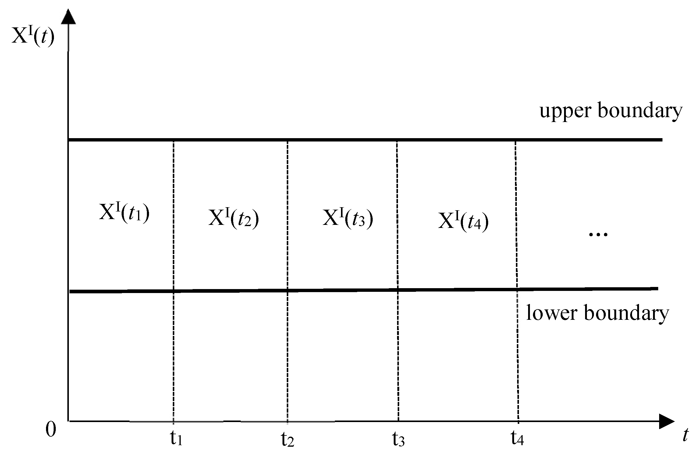
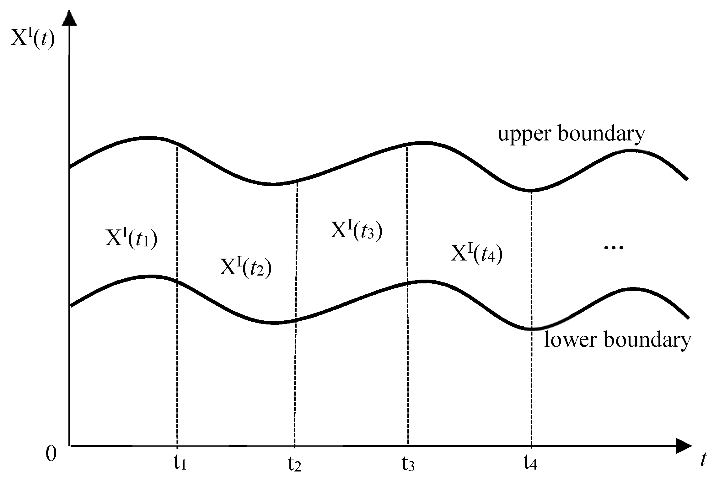
2.1. Basic Theory of Non-random Process

A traditional random process means a corresponding random variable defined at each point of a parameter set, and the magnitude of the value constantly changes with time t. Thus, the result of an observation for the whole process of change is a function of time t [24]. The non-probabilistic convex model process is used to describe the uncertainty excitation. Therefore, the convex model process is used to describe the non-random process. Two boundary curves are used to define the time-varying uncertainty of the parameters, which greatly reduces the dependence of the sample. Thus, this provides an effective mathematical tool for the analysis of structural time-variation and dynamic uncertainty with insufficient parameter information.

The convex model process is defined as [25]:

$$\begin{array}{c}\forall t_i\in T,i=1,2,3\cdots n\\ X\left(t_i\right)=\left[X_{\mathrm{L}},X_{\mathrm{U}}\right]\end{array}$$

(1)

where $X\left(t_i\right)$ is an interval at any time; $X_{\mathrm{L}}$ is the lower boundary of the interval; and $X_{\mathrm{U}}$ is the upper boundary of the interval.

All possible types and shapes of the indeterminate process $X\left(t_i\right)$ would be included in the area consisting of the upper and lower boundaries, as shown in Figure 1. When the convex model is one-dimensional, it is an interval model.

The convex model consists of three numerical characteristics: interval midpoint $X_{\mathrm{C}}$, interval radius $X_{\mathrm{R}}$, and coefficient of variation ${\eta }_x$, which have the following expressions:

$$X_{\mathrm{C}}\left(t\right)=\frac{X_{\mathrm{L}}(t)+X_{\mathrm{U}}(t)}{2}$$

(2)

$$X_{\mathrm{R}}\left(t\right)=\frac{X_{\mathrm{U}}(t)-X_{\mathrm{L}}(t)}{2}$$

(3)

$${\eta }_x=\frac{X_{\mathrm{C}}(t)}{X_{\mathrm{R}}(t)}$$

(4)

where $X_{\mathrm{C}}$ is the interval midpoint, described the magnitude relating to time; $X_{\mathrm{R}}$ is the interval radius, represented the change of the amplitude; and ${\eta }_x$ is the coefficient of variation function, indicating the uncertainty level.

2.2. Non-stationary Non-random Process Model for Seismic Loads

From a statistical point of view, the random process of earthquakes is divided into stationary random process and non-stationary random process [24]. The non-random process is divided into stationary non-random process and non-stationary non-random process [26]. The random process relies on a large sample, however the non-random process only focuses on the boundary of the vibration process, which provides an effective solution to the vibration analysis with insufficient information. Indeed, compared to the huge computational complexity of random processes, the analysis of non-random processes involves less computational work, and therefore also has lower computational costs.

In stationary random process, the median function and the radius function are constant and the autocorrelation function and the autocorrelation coefficient function are only related to time interval $\tau$ and are independent of time t. The stationary non-random process is shown in Figure 2, and its definition can be expressed as follows:

$$X_{\mathrm{C}}\left(t\right)=K_1$$

(5)

$$X_{\mathrm{r}}\left(t\right)=K_1$$

(6)

$$\mathrm{cov}\left(x_1,x_2\right)=K\left(\tau \right)$$

(7)

$${\rho }_{x_1{x}_2}=\rho \left(\tau \right)$$

(8)

where $K_1$ and $K_2$ are constants; $\tau$ is the gap time; and $C\left(\tau \right)$ and $\rho \left(\tau \right)$ are functions of $\tau$.

However, the practical earthquake load has irregular movement and is a non-stationary process in statistics. Non-stationary non-random process refers to all possible types and shapes in the interval of the upper and lower boundary envelopes, as shown in Figure 2. Hence, the non-random process can be defined as:

$$\begin{array}{c}\mathrm{If}\forall X_i^I\in \psi \\ \mathrm{Then}{X}^I\left(t\right)=\left(X_1^I\left(t\right),X_2^I\left(t\right),\cdots ,X_n^I\left(t\right)\right)\end{array}$$

(9)

where $\psi$ is a convex process model.

According to the random characteristics of non-stationarity in practical earthquake, the non-stationary model of the uniform modulation process can be expressed as:

$$y\left(t\right)=g\left(t\right)X\left(t\right)$$

(10)

where $X\left(t\right)$ is the stationary interval process of ground motion; and $g\left(t\right)$ is the three-stage non-stationary envelope function, which has the following expression [27]:

$$g\left(t\right)=\{\begin{array}{l}{\left(t/t_1\right)}^2,0\le t<t_1\\ 1,t_1\le t<t_2\\ e^{-c\left(t-t_2\right)},t_2\le t\end{array}$$

(11)

where $c$ is a constant; and $t_1$ and $t_2$ are the rise time and fall time of the peak, respectively.

3. Dynamic Analysis of Buried Pressure Pipelines

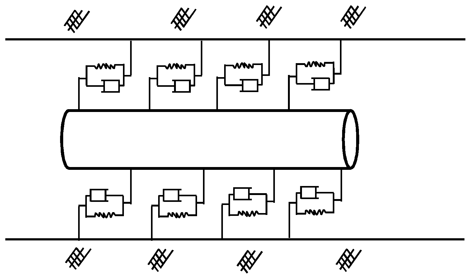
3.1. Seismic Response of Buried Pipelines

Research and seismic damage records show that the axial influence of buried pipelines subjected to seismic loading is much greater than the lateral impact [27,28,29]. Therefore, this paper only considers the axial seismic behavior of the pipeline. When the random process is processed as an interval process based on the analysis of the non-random vibration, the response of the structure should have forms of intervals with upper and lower bounds [25]. With limited sample information of excitation, the non-random vibration method can reduce the dependence on the sample and provide feasible guidance for seismic research of pipelines with lack of information.

The interaction between soil and pipeline is modeled by using a nonlinear Winkler Foundation model, in which the interaction behavior is represented by nonlinear discrete soil springs and dampers. The basic assumption for the interaction of soil and pipeline can be summarized as follows:

(1) It is assumed that the site conditions and the soil parameters are unchanged along the pipelines;

(2) The pipe damping is extremely small compared to the soil damping of the foundation. Therefore, the material damping of the pipeline itself can be ignored;

(3) The soil around a pipeline is simplified as a continuously uniform distributed damper and spring as shown in Figure 3.

Since a pipeline is a long-span structure, it is necessary to consider the temporal and spatial changes of the ground motion. Combined with the previous analysis, the axial dynamic equation for establishing a pipeline suffered from earthquake has the following form:

$$m\ddot{u}\left(x,t\right)+c\dot{u}\left(x,t\right)+ku\left(x,t\right)-K\frac{\partial u\left(x,t\right)}{\partial x^2}=k{u}_{\mathrm{g}}\left(x,t\right)+c{\dot{u}}_{\mathrm{g}}\left(x,t\right)$$

(12)

where $m$ is the weight of the pipeline; $c$ is the damping coefficient of the medium around the pipeline; $k$ is the stiffness coefficient around the pipeline; $K$ is the axial stiffness of the pipeline; $x$ is the axial coordinate of the pipeline; $u_g\left(x,t\right)$ is the axial displacement of the site subjected to earthquake; and $u\left(x,t\right)$ is the axial displacement of the pipeline.

Research has shown that the axial displacement of a pipeline is the sum of the static displacement caused by the site and the dynamic displacement caused by the inertia and damping of the pipeline [30,31]. Based on the series solution of buried pipeline with multipoint excitation, dynamic displacement can be represented as:

$$u_{\mathrm{D}}\left(x,t\right)={\displaystyle \sum _{i=0}^{\infty }{q}_i}\left(t\right)\cos \frac{i\pi x}{l},i=0,1,2,3\cdots \infty$$

(13)

where $u_{\mathrm{D}}\left(x,t\right)$ is the dynamic displacement changing with time; $l$ is the length of the pipeline; and $q_i\left(t\right)$ is the generalized coordinate, which can be obtained according to the decomposition of vibration mode.

The analytical solution of generalized coordinates has the following expression:

$$\{\begin{array}{l}{q}_0\left(t\right)=\frac{1}{2{\omega }_0}{\displaystyle {\int }_0^l\exp \left[{\xi }_0{\omega }_0\left(t-\tau \right)\right]}{\ddot{a}}_0\left(t\right)\sin {\omega }_0\left(t-\tau \right)d\tau \\ q_i\left(t\right)=\frac{1}{{\omega }_i}{\displaystyle {\int }_0^l\exp \left[{\xi }_i{\omega }_i\left(t-\tau \right)\right]}{\ddot{a}}_i\left(\tau \right)\sin {\omega }_i\left(t-\tau \right)d\tau ,i=1,2,3\cdots n\end{array}$$

(14)

where ${\xi }_i$ is the damping ratio corresponding to the i-th mode of vibration; and ${\omega }_i$ is the damped vibration frequency of the pipeline, which can be expressed as $\sqrt{\left(\frac{i^2{\pi }^{2}K}{l^{2}m}+\frac{k}{m}\right)\left(1-{\xi }_i^2\right)}$.

As mentioned before, in the response of the pipeline, static displacement is caused by site displacement. By taking static analysis into consideration, its equation can be constructed and has the following form:

$$k{u}_{\mathrm{S}}\left(x,t\right)-K\frac{\partial u_{\mathrm{S}}\left(x,t\right)}{\partial x^2}=k{u}_{\mathrm{g}}\left(x,t\right)$$

(15)

where $u_{\mathrm{S}}\left(x,t\right)$ is the static displacement.

Based on the theory of series solution, the equation of static displacement is given by [30,31]:

$$u_{\mathrm{S}}\left(x,t\right)=\frac{1}{l}{\displaystyle {\int }_0^l{u}_{\mathrm{g}}\left(x,t\right)xdx}+{\displaystyle \sum _{i=0}^{\infty }\frac{\frac{2k}{l}{\displaystyle {\int }_0^l{u}_{\mathrm{g}}\left(x,t\right)\cos \frac{i\pi x}{l}dx}}{k+K\frac{i^2{\pi }^2}{l^2}}}\cos \frac{i\pi x}{l}$$

(16)

To obtain the more actual stress response, the axial displacement of the pipeline subjected to earthquake can be expressed as:

$$\begin{array}{l}u\left(x,t\right)=u_{\mathrm{S}}\left(x,t\right)+u_{\mathrm{D}}\left(x,t\right)\\ =\frac{1}{l}{\displaystyle {\int }_0^l{u}_{\mathrm{g}}\left(x,t\right)xdx}+{\displaystyle \sum _{i=0}^{\infty }\frac{\frac{2k}{l}{\displaystyle {\int }_0^l{u}_{\mathrm{g}}\left(x,t\right)\cos \frac{i\pi x}{l}dx}}{k+K\frac{i^2{\pi }^2}{l^2}}}\cos \frac{i\pi x}{l}+{\displaystyle \sum _{i=0}^{\infty }{q}_i}\left(t\right)\cos \frac{i\pi x}{l},i=0,1,2,\cdots ,\infty \end{array}$$

(17)

where $u\left(x,t\right)$ is the total axial displacement of the pipeline.

The strain of the pipeline can be obtained by using the relationship between stress and deformation, which is given by:

$$\epsilon =\frac{1}{l^2}{\displaystyle {\int }_0^l{u}_{\mathrm{g}}\left(x,t\right)dx}+{\displaystyle \sum _{i=0}^{\infty }\frac{\frac{2k}{l^2}{\displaystyle {\int }_0^l{u}_{\mathrm{g}}\left(x,t\right)\cos \frac{i\pi x}{l}dx}}{k+K\frac{i^2{\pi }^2}{l^2}}}\cos \frac{i\pi x}{l}+\frac{1}{l}{\displaystyle \sum _{i=0}^{\infty }{q}_i}\left(t\right)\cos \frac{i\pi x}{l},i=0,1,2,\cdots ,\infty$$

(18)

where $\epsilon$ is the strain of the pipeline.

Therefore, the stress on a pipeline subjected to earthquake can be obtained by establishing the following equation:

$$\sigma =\frac{E}{l^2}{\displaystyle {\int }_0^l{u}_{\mathrm{g}}\left(x,t\right)dx}+{\displaystyle \sum _{i=0}^{\infty }\frac{\frac{2kE}{l^2}{\displaystyle {\int }_0^l{u}_{\mathrm{g}}\left(x,t\right)\cos \frac{i\pi x}{l}dx}}{k+K\frac{i^2{\pi }^2}{l^2}}}\cos \frac{i\pi x}{l}+\frac{E}{l}{\displaystyle \sum _{i=0}^{\infty }{q}_i}\left(t\right)\cos \frac{i\pi x}{l},i=0,1,2,\cdots ,\infty$$

(19)

where $E$ is the elastic modulus.

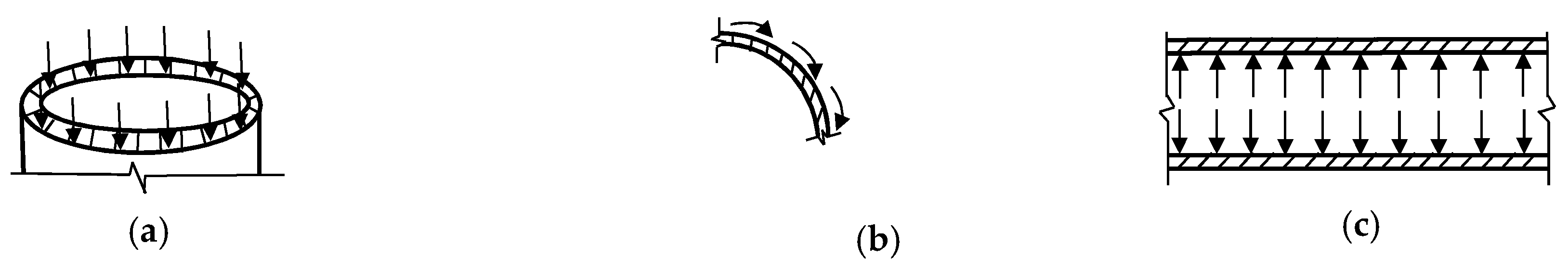
3.2. Response of Buried Pressure Pipelines based on Fourth Strength Theory

When a buried pipeline is only subjected to internal pressure, the pipeline produces circumferential stress, axial stress, and radial stress, as shown in Figure 4. However, the long-distance buried pipeline is a thin-walled structure in this paper. Thus, the radial stress can be ignored, and the expression of three directions can be expressed as [32,33]:

$${\sigma }_{\mathrm{c}}=\frac{PD}{2w}$$

(20)

$${\sigma }_{\mathrm{a}}=\frac{\nu PD}{2w}$$

(21)

$${\sigma }_{\mathrm{r}}=0$$

(22)

where ${\sigma }_{\mathrm{c}}$ is the circumferential stress; ${\sigma }_{\mathrm{r}}$ is the radial stress; ${\sigma }_{\mathrm{a}}$ is the axial stress; $D$ is the diameter; $w$ is the wall thickness of the pipeline; and $\nu$ is the Poisson ratio.

Strength theory is used to determine whether a material is broken under complex stress conditions. The fourth strength theory, also known as energy theory of the maximum shape-change, can determine the conditions of plastic failure [34]:

$${\sigma }_{\mathrm{s}}=\sqrt{\frac{1}{2}\left[{\left({\sigma }_1-{\sigma }_2\right)}^2+{\left({\sigma }_2-{\sigma }_3\right)}^2+{\left({\sigma }_3-{\sigma }_1\right)}^2\right]}$$

(23)

where ${\sigma }_{\mathrm{s}}$ is the Von Mises stress; and ${\sigma }_1$, ${\sigma }_2$, and ${\sigma }_3$ are stresses in three main stresses, respectively.

Then, the axial stress on the pipeline can be expressed as the joint effect of the axial stress on the pipeline subjected to earthquake and the axial stress with the internal pressure:

$${\sigma }_{\mathrm{A}}={\sigma }_{\mathrm{e}}+{\sigma }_{\mathrm{a}}$$

(24)

The Von Mises stress can be obtained by combining ${\sigma }_{\mathrm{A}}$, ${\sigma }_{\mathrm{r}}$, and ${\sigma }_{\mathrm{c}}$, in the following form:

$${\sigma }_{\mathrm{s}}=\sqrt{\left({\sigma }_{\mathrm{c}}^2-{\sigma }_{\mathrm{A}}{\sigma }_{\mathrm{c}}+{\sigma }_{\mathrm{A}}^2\right)}$$

(25)

4. Seismic Damage Assessment based on Cloud Model

4.1. Theory of Cloud Model

The assessment of seismic damage to pipelines has randomness and fuzziness. Since the concept of the damage degree of pipelines is fuzzy and the stress values obtained by dynamic response are uncertain, we introduce the concept of cloud to express the randomness and fuzziness through graphical features. The concept of cloud realizes the mutual transformation of qualitative and quantitative, and solves the evaluation result of boundary ambiguity and overlap.

Suppose that $U$ is a quantitative domain of exact numerical representation, and $C$ is a qualitative concept on $U$. For a quantitative value $x\in U$, the membership degree $u_c\left(x\right)$ is a description of the qualitative concept represented by $x$ for $C$. Thus, the distribution of membership degrees on the domain $U$ is called the cloud. The value range of $u_c\left(x\right)$ is $\left[0,1\right]$ and the cloud is a mapping from the domain $U$ to the interval $\left[0,1\right]$, which can be expressed as [35]:

$$u:U\to \left[0,1\right],\forall x\in U,x\to u\left(x\right)$$

(26)

Each x is defined as a cloud drop, which is a quantitative description of a qualitative concept, and all the cloud drops are gathered into a cloud. The deterministic levels of different clouds reflect different ambiguities. Additionally, the cloud drop itself represents a random value. Therefore, the accuracy of the qualitative description depends on the number of clouds. For example, each cloud drop, as shown in Figure 5, represents the degree of certainty of the concept, indicating the quantitative position of the qualitative concept in the numerical space. Thus, the assessment value denotes that the value corresponding to the different evaluation of the object, and the certainty grade is the degree of membership.

The cloud model uses the "cloud" to define the fuzziness and randomness of the data, constituting a transition between qualitative and quantitative. The three numerical characteristics of the cloud model are expectation $E_x$, entropy $E_n$, and super-entropy $H_e$, which are quantitative concepts to describe the concept of qualitative. The evaluation results of the cloud model expression give the position of evaluated central value through the expectation, and the entropy and super-entropy express the randomness and dispersion of the evaluation results. Therefore, the evaluation results are more objective and accurate. The description of numerical characteristics for expectation, entropy, and super-entropy are shown in Figure 6, Figure 7 and Figure 8, respectively.

This paper establishes a cloud model-based approach to solve the uncertainty and fuzziness of structural damage assessment, and the damage evaluations of the pipeline with non-random earthquake are explained by the numerical characteristics of the model. Expectation is a qualitative description of a representative sample. In this paper, expectation represents the value of pipeline damage, which reflects the extent of damage. The entropy is used to measure the degree of uncertainty, and represents the measurability of qualitative concepts. Moreover, the entropy represents the range of values that can be accepted by the qualitative concept, which is a measure of the qualitative concept, and it is the fuzzy measure and the degree of dispersion of qualitative concept, reflecting the degree of damage and the degree of dispersion of the stress values at each point of each pipeline relative to the evaluation stress value in this paper. The super-entropy is a measure of uncertainty state, reflecting the degree of aggregation of stress value. Therefore, the expectation gives the location of the evaluation center value, and the randomness and discreteness of the evaluation results are represented by entropy and super-entropy.

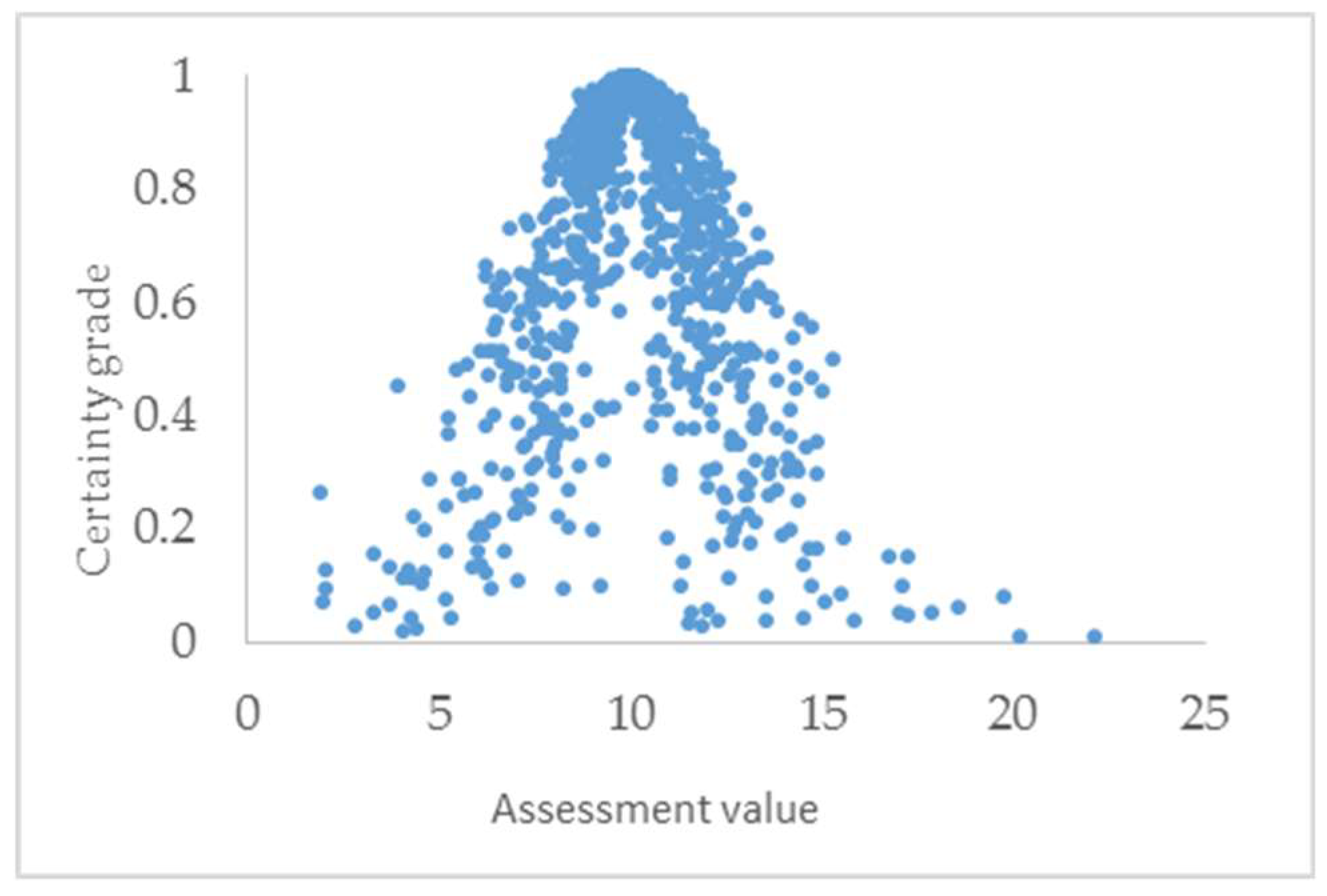
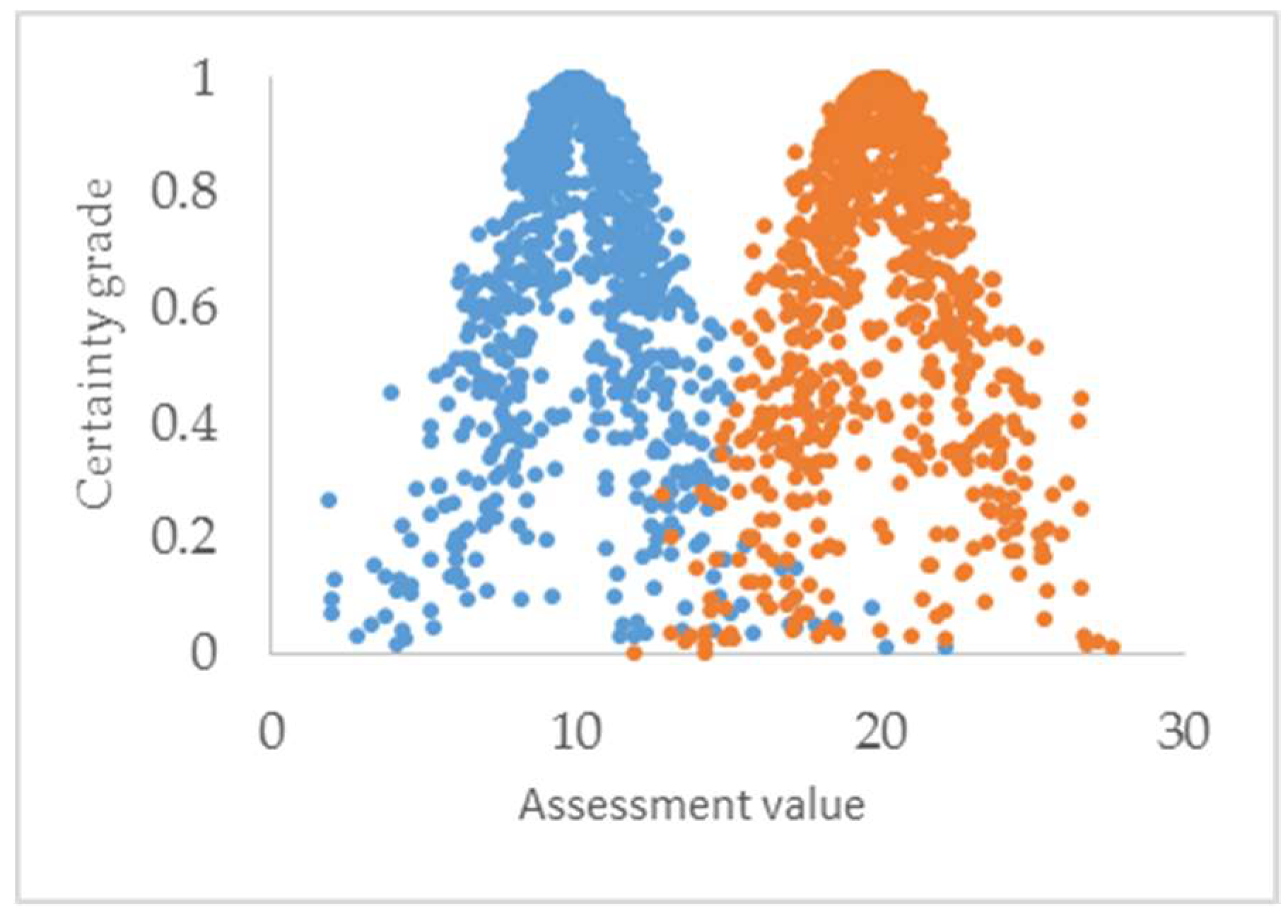
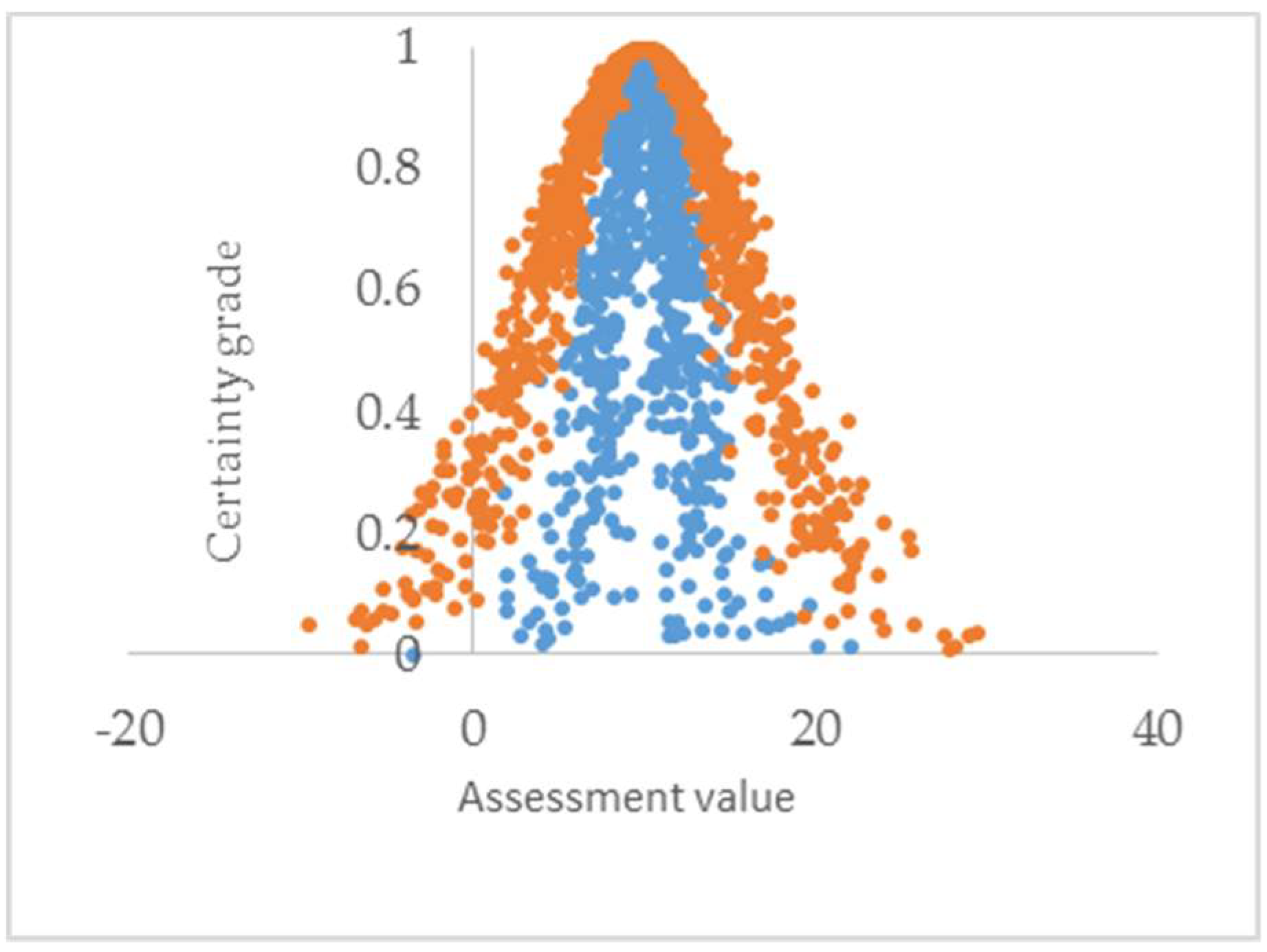
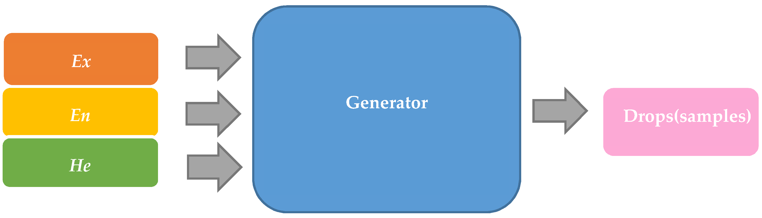
4.2. Damage Samples based on Normal Forward Cloud Generator

A normal cloud generator essentially reflects the mapping between qualitative and quantitative, and is a specific algorithm from the random and fuzzy data. Furthermore, the membership degree is based on the normal distribution of probability theory and the clock-row membership function in the fuzzy set.

According to the definition of a positive normal cloud, the generator can produce the required m drops when the three quantitative features ($E_x$, $E_n$, and $H_e$) and the required number of cloud drops are known. A diagram of the algorithm of the forward cloud generator is shown in Figure 9. For clarity, the procedure of the normal cloud generator algorithm is described as follows [36,37]:

(1) Generate a normal random number, $E_n^{\prime }=N\left(E_n,H_e^2\right)$, where $E_n$ is the expected value and $H_e^2$ is the standard deviation;

(2) Generate a normal random number, $x_i=N\left(E_x,H_{n_i}^{\prime 2}\right)$, where $E_x$ is the expected value and $H_{n_i}^{\prime 2}$ is the standard deviation;

(3) $x$ is a specific quantitative value of qualitative concept $C$, which can be calculated by equation (27) to determine the quantitative value of the qualitative value:

$$u\left(x\right)=\exp \left(-\frac{{\left(x-E_x\right)}^2}{2{\left(E_n^{\prime }\right)}^2}\right)$$

(27)

(4) Repeat steps (1) to (3) to generate n cloud drops. Therefore, a cloud model through the cloud drops is drawn.

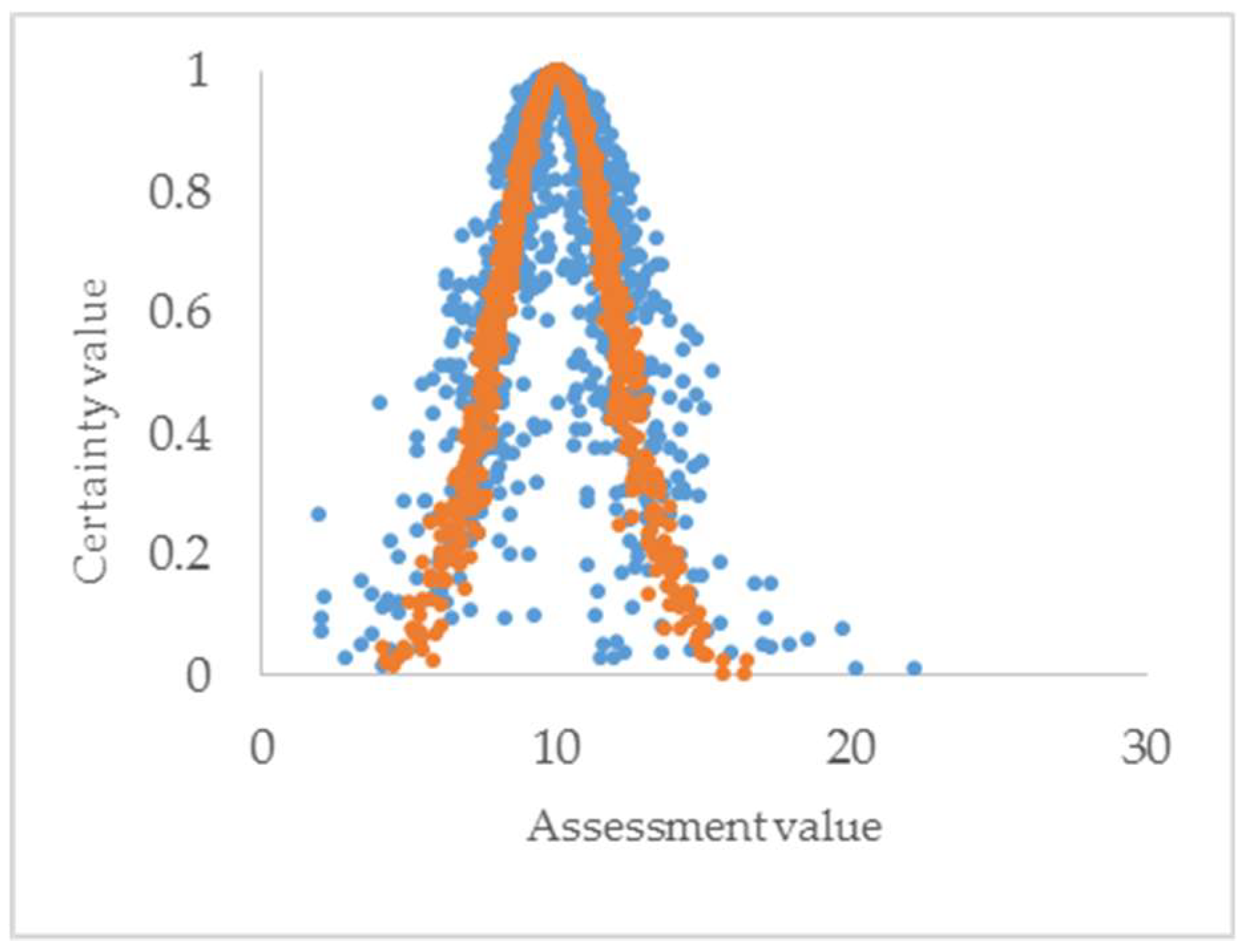
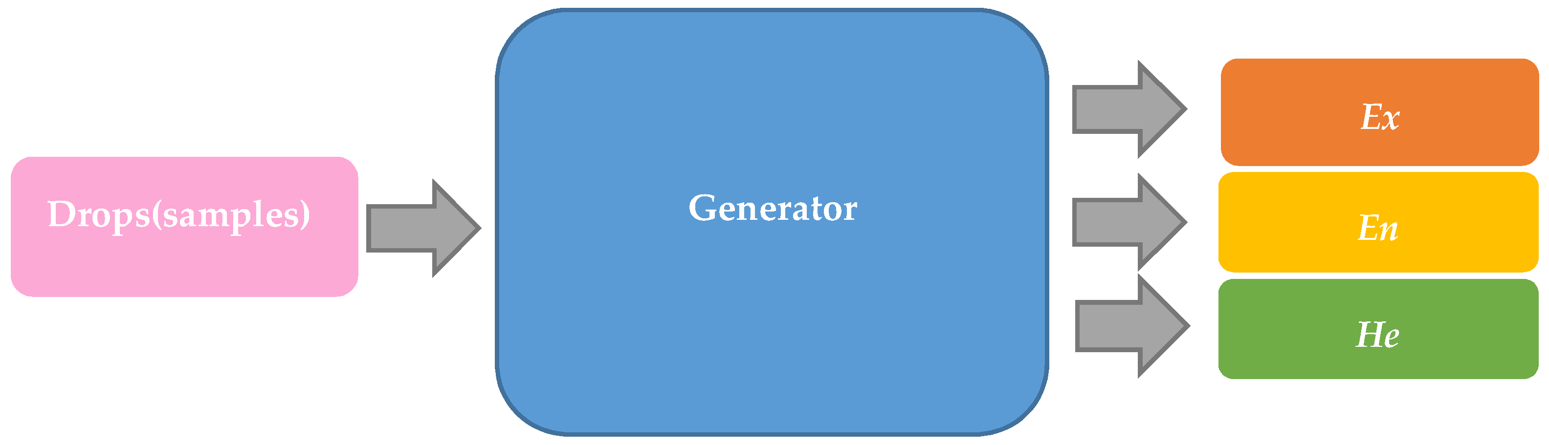
4.3. Damage Samples based on Normal Backward Cloud Generator

In contrast to the forward cloud generator, three quantitative characteristics of the cloud model ($E_x$, $E_n$, and $H_e$) can be obtained through the cloud drops, as shown in Figure 10. The steps of the normal cloud generator algorithm are constructed as follows:

(1) Calculate the sample mean $\overline{X}$, the absolute central distance of the first order sample $S^2$, and sample variance $S^2$ from sample point $x_i\left(i=1,2,3\cdots n\right)$:

$$\overline{X}=\frac{1}{m}{\displaystyle \sum _{i=1}^m{x}_i}$$

(28)

$$M=\frac{1}{m}{\displaystyle \sum _{i=1}^m\left|x_i-\overline{X}\right|}$$

(29)

$$S^2=\frac{1}{m-1}{{\displaystyle \sum _{i=1}^m\left(x_i-\overline{X}\right)}}^2$$

(30)

(2) Obtain expressions of quantitative characteristics ($E_x$, $E_n$ and $H_e$):

$$E_x=\overline{X}$$

(31)

$$E_n=n\sqrt{\frac{\pi }{2}}{\displaystyle \sum _{i=1}^n\left|x_i-E_x\right|}$$

(32)

$$H_e=\sqrt{S^2-E_n^2}$$

(33)

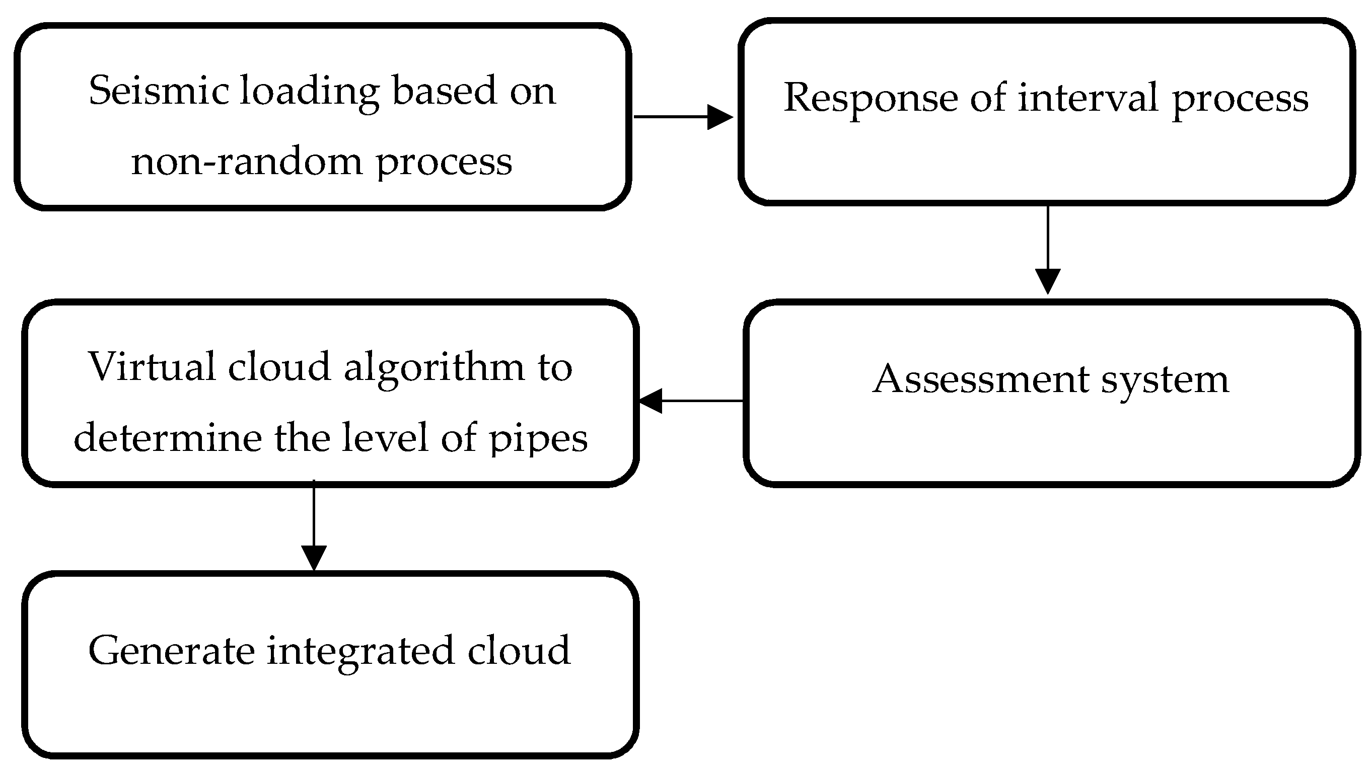
4.4. Assessment Process

The traditional seismic analysis for pipeline takes a section of pipeline as the research object and obtains the stress response of the pipeline. The stress value determined by the section corresponds to the yield limit stress of the material as an evaluation of the damage. Finally, the damage of the pipeline is evaluated by comparing the stress values determined by the section with the yield limit stress of the material. However, when a buried pipeline is subjected to earthquake, the degree of damage to the pipeline and its uncertainty cause randomness and fuzziness in the evaluation process. Thus, it is necessary to establish a method for determining the seismic damage to pipelines, which is mainly to solve the evaluation indicators of fuzziness and randomness in seismic damage assessment of pipelines.

Referring to the classical division of damage to pipelines, the grades of damage can be expressed as:

$$U=\left[U_1,U_2,U_3,U_4,U_5\right]$$

(34)

where $U_1$ represents essential integrity; $U_2$ represents minor damage; $U_3$ represents medium damage; $U_4$ represents severe damage; and $U_5$ represents destruction.

According to the three states of failure criteria and interval theory, this paper establishes a new evaluation norm, as shown as

Table 1. Division of degree of damage to pipelines.

Grades of Damage	Description	Indices
essential integrity	good condition	$\sigma <\left[{\sigma }_{\mathrm{r}}\right]$
minor damage	non-destructive or appears micro-cracks locally.	$\left[{\sigma }_{\mathrm{r}}\right]<\sigma <\frac{\left[{\sigma }_{\mathrm{b}}\right]+2\left[{\sigma }_{\mathrm{r}}\right]}{3}$
medium damage	joint fracture, local deformation or cracking of weld seam, slight leakage	$\frac{\left[{\sigma }_{\mathrm{b}}\right]+2\left[{\sigma }_{\mathrm{r}}\right]}{3}<\sigma <\frac{2\left[{\sigma }_{\mathrm{b}}\right]+\left[{\sigma }_{\mathrm{r}}\right]}{3}$
severe damage	severe deformation or fracture, cracked weld, heavy leakage, difficult to repair	$\frac{2\left[{\sigma }_{\mathrm{b}}\right]+\left[{\sigma }_{\mathrm{r}}\right]}{3}<\sigma <\left[{\sigma }_{\mathrm{b}}\right]$
destruction	breakage, severe damage to the interface weld, severe leakage, no repair value	$\left[{\sigma }_{\mathrm{b}}\right]<\sigma$

¹${\sigma }_{\mathrm{r}}$ is the ultimate compressive strength; ${\sigma }_{\mathrm{b}}$ is the ultimate tensile strength.

. By taking cloud model into consideration, the result of assessment is a bilateral constraint, $\left[a,b\right]$, and the cloud parameter computation equations are given by [22]:

$$E_x=\frac{a+b}{2}$$

(35)

$$E_n=\frac{a+b}{6}$$

(36)

$$H_e=k$$

(37)

where $a$ is the lower boundary of the interval; $b$ is the upper boundary of the interval; and $k$ is a constant adapting to fuzzy comments.

To assess the safety of pipelines, the procedure of the assessment method is proposed as shown in Figure 11. First, the response of interval through non-random process can be obtained. Second, the assessment system of pipelines depends on the material of the pipeline being established. Third, the evaluation chart can be established based on cloud model by combining the calculated results with cloud algorithm. Last, the integrated cloud inference results can be shown intuitively by adding the practical response of the pipeline.

5. Example

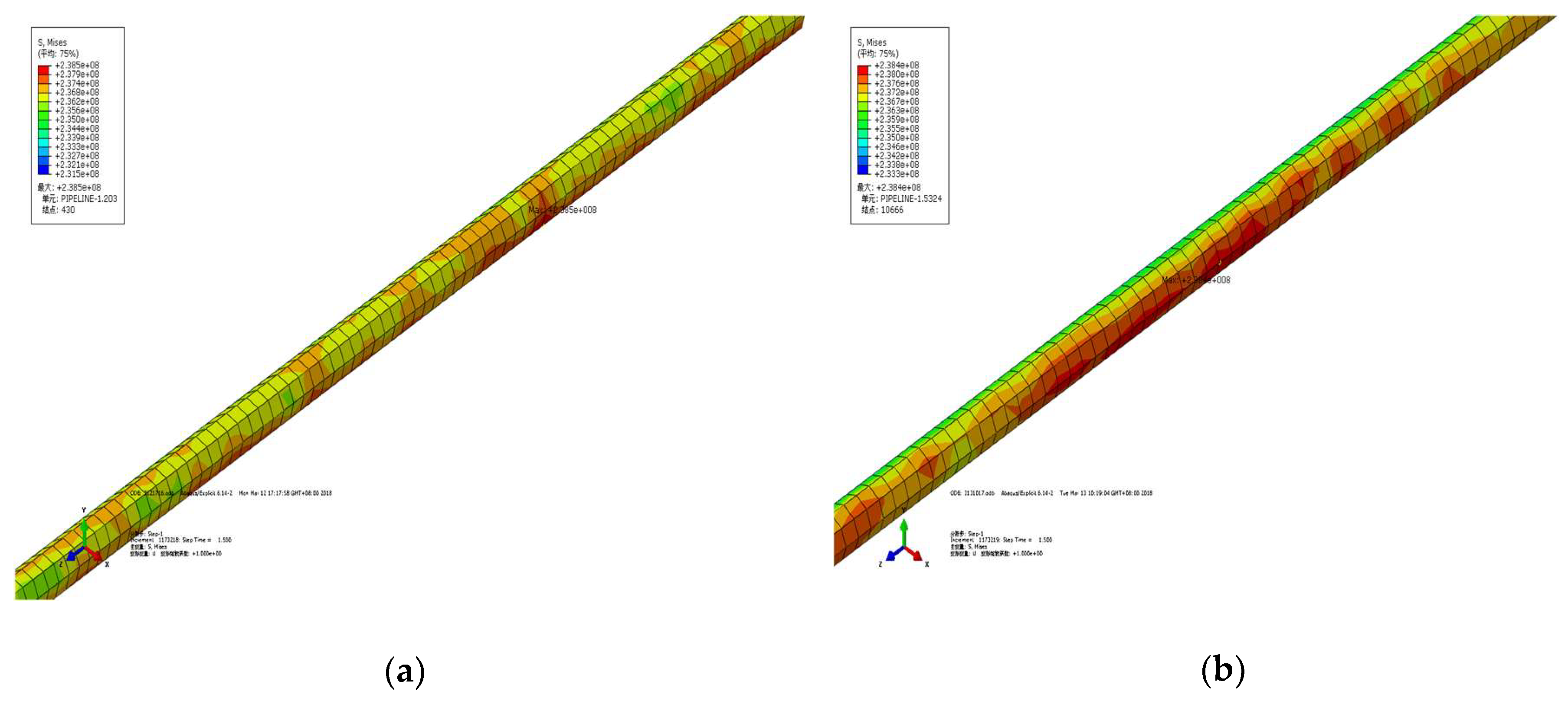
5.1. Calculation Based on Finite Element

As an example, this paper establishes a model of a pipeline that suffers from the seismic excitation of a non-random process. The length of the pipeline is 200 m and the material of the pipeline is X60 steel. By using Abaqus (Dassault aircraft company, Vaucresson, France), a finite element software, a three-dimensional finite element model of pipe–soil interaction is established by nonlinear surface-to-surface contact. The outer wall of the pipeline with high rigidity is selected as the main surface, and the soil with small rigidity is selected as the surface. The normal contact behavior adopts “penalty”, and the friction coefficient is 0.5. The soil is simulated by a solid element with a depth of 3 m and the constitutive relation is the Drucker–Prager (D-P) model. The mechanical properties of X60 refer to literature [38], and the basic parameters of the materials are shown in

Table 2. Basic parameters of materials.

Type of Material	Density/(kg·m−3)	Elastic Modulus/Pa	Poisson Ratio	Expansion Angle/°	Friction Angle/°	Flow Stress Ratio
Soil	1867.3	2 $\times$ 108	0.4	28.7	18.4	0
Pipeline	7850.0	2.07 $\times$ 1011	0.3	—	—	—

.

After applying the load, as shown in Equation (38) [39,40], the Von Mises response of the pipeline can be obtained by using the finite element calculation, as shown in Figure 12. By combining with theoretical analysis, the result of the interval of response is taken as: [229.63 MPa, 242.28 MPa].

$$g_{}\left(t\right)=\{\begin{array}{l}\left[-4.671{\left(t/5\right)}^2,3.417{\left(t/5\right)}^2\right],0\le t<5\\ \left[-4.671,3.417\right],5\le t<10\\ \left[-4.671e^{-0.3\left(t-10\right)},3.417e^{-0.3\left(t-10\right)}\right],t_2\le 10\end{array}$$

(38)

5.2. Damage Assessment of a Pipeline

When the stress interval value is obtained, the cloud model map at this time can be obtained by the forward cloud generator, and the degree of damage to the pipeline can be obtained by comparing the standard assessment figure of the pipeline damage. According to the assessment of stress grades, the standard assessment model for seismic damage is proposed based on cloud model, which is shown in Figure 13a, and combined with the stress response of the pipeline with seismic excitation of non-random process. The evaluation is shown in Figure 13b. The result indicates that the degree of damage to the pipeline is “essentially intact”. When the stress interval is [380 MPa, 430 MPa], the damage degree is between “essentially intact” and “minor damage”, as shown in Figure 13c.

When the maximum stress values of the pipeline are analyzed, the assessment method is proposed to describe the fuzziness of the damage and understand the degree of dispersion visually. Thus, the broad abscissa demonstrates the fuzziness of the results and the advantages of the concept randomness, making the evaluation results more abundant, and it can more accurately describe the degree of structural damage. Hence, the degree of structural damage is a process from intact to damaged and the randomness of concept. From the distribution of the data, the evaluation center can be seen the location. Moreover, the discreteness and randomness of the results can be expressed by entropy and super-entropy, which makes the results more accurate. Clearly, for the operation of the pipeline in the future, it is necessary to improve the maintenance and assessment method of the pipeline to avoid secondary accident.

6. Conclusion

Since pipelines are the most important transportation structures for energy generation, it is necessary to assess their safety after an earthquake. By considering the insufficient data from seismic records, this paper proposes to analyze the response of buried pressure pipelines based on non-random process. As the degree of damage to a pipeline is not a definite value, but rather is ambiguous, it is difficult to assess, and the stress values of pipelines have an indeterminate range owing to non-random excitation. However, combined with the established standard cloud chart, cloud inference can implement the transition between quantitative description and qualitative concept. Moreover, this method can also solve the evaluation of interval response referring to the uncertainties and fuzziness in the damage assessment process. The following conclusions can be obtained by the analysis of the example in this paper:

• The seismic excitation with small data is investigated by using non-random process, and the response of pipeline exposed to earthquake can be obtained.
• For the design of buried pressure pipeline, the result of dynamic response boundary is easier for engineers to understand. Therefore, it can be used as a supplement of random process excitation.
• Combined with the response of non-random process, the method to realize fuzziness and randomness of interval sample is proposed, and it achieves the conversion between quantitative and qualitative. Thus, this method can effectively reduce the impact of human factors in the assessment process and can accurately describe the intermediate state of pipeline damage and the uncertainty of pipeline stress.
• The damage model of the pipeline based on cloud model established here can more reasonably describe the damage of the structure with a certain level, and the assessment result is shown visually using a cloud chart. This approach has laid the foundation for the safety evaluation of seismic engineering with small sample in the future.

References

1. Hu, G.; Zhang, P.; Wang, G.; Zhang, M.; Li, M. The Influence of Rubber Material on Sealing Performance of Packing Element in Compression Packer. J. Nat. Gas. Sci. Eng. 2017, 38, 120–138. [Google Scholar] [CrossRef]
2. Zhang, P.; Qin, G.; Wang, Y. Optimal Maintenance Decision Method for Urban Gas Pipelines Based on as Low as Reasonably Practicable Principle. Sustainability 2019, 11, 153. [Google Scholar] [CrossRef]
3. Li, D.S.; Lu, D.; Hou, Y.L. Pipeline Damage Identification Based on Additional Virtual Masses. Appl. Sci. 2017, 7, 1040. [Google Scholar] [CrossRef]
4. Martini, A.; Rivola, A.; Troncossi, M. Autocorrelation Analysis of Vibro-Acoustic Signals Measured in a Test Field for Water Leak Detection. Appl. Sci. 2018, 8, 2450. [Google Scholar] [CrossRef]
5. Martini, A.; Troncossi, M.; Rivola, A. Leak Detection in Water-Filled Small-Diameter Polyethylene Pipes by Means of Acoustic Emission Measurements. Appl. Sci. 2017, 7, 2. [Google Scholar] [CrossRef]
6. EPA—United States Environmental Protection Agency. Control and Mitigation of Drinking Water Losses in Distribution Systems; EPA 816-R-10-019 Report; United States Environmental Protection Agency: Washington, DC, USA, 2010.
7. Xu, C.; Gong, P.; Xie, J.; Shi, H.; Chen, G.; Song, G. An acoustic emission based multi-level approach to buried gas pipeline leakage localization. J. Loss Prev. Process Ind. 2016, 44, 397–404. [Google Scholar] [CrossRef]
8. Nedjati, A.; Vizvari, B.; Izbirak, G. Correction to: Post-earthquake response by small UAV helicopters. nat. Hazard. 2018, 90, 511. [Google Scholar] [CrossRef]
9. Feng, Q.S.; Chen, J.F.; Ai, M.Y.; Cui, T.; Han, X.M. Application of Pipeline Integrity Technology in Earthquake Disaster. Acta Petrolei Sinica 2010, 31, 139–143. [Google Scholar] [CrossRef]
10. Scawthorn, C.; Yanev, P.I. 17 January 1995, Hyogo–ken Nambu, Japanese Earthquake. Eng. Struct. 1995, 17, 146–157. [Google Scholar] [CrossRef]
11. Hwang, H.; Chiu, Y.H.; Chen, W.Y.; Shih, B.J. Analysis of Damage to Steel Gas Pipelines Caused by Ground Shaking Effects during the Chi-Chi, Taiwan Earthquake. Earthquake Spectra 2004, 20, 1095–1110. [Google Scholar] [CrossRef]
12. Hindy, A.; Novak, M. Earthquake Response of Underground Pipelines. Earthquake Eng. Struct. Dyn. 2010, 7, 451–476. [Google Scholar] [CrossRef]
13. Wang, L.R.L.; Cheng, K.M. Seismic Response Behavior of Buried Pipelines. J. Press. Vessel Technol. 1979, 101, 21–30. [Google Scholar] [CrossRef]
14. Li, Y.; Zhang, Y.H. Random Seismic Analysis of Multi-Supported Pipelines Subjected to Spatially Varying Ground Motions. Appl. Math. Mech. 2015, 36, 582–592. [Google Scholar] [CrossRef]
15. Lee, D.H.; Kim, B.H.; Lee, H.; Kong, J.S. Seismic Behavior of a Buried Gas Pipeline under Earthquake Excitations. Eng. Struct. 2009, 31, 1011–1023. [Google Scholar] [CrossRef]
16. Ben-Haim, Y.; Elishakoff, I. Convex Models of Uncertainties in Applied Mechanics; Elsevier Science: Amsterdam, Netherlands, 1990. [Google Scholar]
17. Qiu, Z.; Wang, X. Parameter Perturbation Method for Dynamic Responses of Structures with Uncertain-but-bounded Parameters based on Interval Analysis. Int. J. Solids Struct. 2005, 42, 4958–4970. [Google Scholar] [CrossRef]
18. Sainz, Á.M.; Armengol, J.; Vehí, J. Fault Detection and Isolation of the Three-tank System Using the Modal Interval Analysis. J. Process. Control. 2002, 12, 325–338. [Google Scholar] [CrossRef]
19. Jiang, C.; Liu, N.Y.; Ni, B.Y.; Han, X. Giving Dynamic Response Bounds under Uncertain Excitations—A Non-Random Vibration Analysis Method. Chin. J. Theor. and Appl. Mech. 2016, 48, 447–463. [Google Scholar] [CrossRef]
20. Sooraj, T.R.; Mohanty, R.K.; Tripathy, B.K. Fuzzy Soft Set Theory and Its Application in Group Decision Making. Adv. Comput. Commun. Technol. 2016, 452, 171–178. [Google Scholar]
21. Li, D.Y.; Du, F. Artificial Intelligence with Uncertainty, 2nd ed.; National Defense Industry Press: Beijing, China, 2014. [Google Scholar]
22. Wang, G.; Xu, C.; Li, D. Generic Normal Cloud Model. Inf. Sci. 2014, 280, 1–15. [Google Scholar] [CrossRef]
23. Dai, C.H.; Zhu, Y.F.; Chen, W.R. Adaptive Probabilities of Crossover and Mutation in Genetic Algorithms Based on Cloud Model. Proc. IEEE Inf. Theor. Workshop 2006, 24, 710–713. [Google Scholar] [CrossRef]
24. Carassale, L. Random Process. as Earthquake Motions; Springer: Berlin, Heidelberg, 2015. [Google Scholar]
25. Liu, N.Y. Non-random Process Model and Non-random Vibration Analysis. Master’s Thesis, Hunan University, Changsha, China, 2016. [Google Scholar]
26. Jiang, C.; Ni, B.Y.; Han, X.; Tao, Y.R. Non-probabilistic convex model process: A New Method of Time-variant Uncertainty Analysis and Its Application to Structural Dynamic Reliability Problems. Comput. Meth. Appl. Mech. Eng. 2014, 268, 656–676. [Google Scholar] [CrossRef]
27. Davenport, A.G. Note on the Distribution of the Largest Value of a Random Function with Application to Gust Loading. Proc. Inst. Civ. Eng. 1964, 28, 187–196. [Google Scholar] [CrossRef]
28. Pineda-Porras, O.; Ordaz, M. A New Seismic Intensity Parameter to Estimate Damage in Buried Pipelines due to Seismic Wave Propagation. J. Earthquake Eng. 2007, 11, 14. [Google Scholar] [CrossRef]
29. Xue, J.H.; Ou, J.P.; Sun, J.Q. Dynamic Analysis of Fluid-conveying Pipelines. World Inf. Earthquake Eng. 2001, 17, 29–32. [Google Scholar] [CrossRef]
30. Ariman, T.; Muleski, G.E. A Review of the Response of Buried Pipelines under Seismic Excitations. Earthquake Eng. Struct. Dyn. 2010, 9, 133–152. [Google Scholar] [CrossRef]
31. Qu, T.J.; Wang, Q.X. Response of Underground Pipeline to Multi-support Longitudinal Excitations. Earthquake Eng. Eng. Vibr. 1993, 4, 39–46. [Google Scholar]
32. Qu, T.J.; Wang, J.J.; Wang, Q.X. A Practical Model for the Power Spectrum of Spatially Variant Ground Motion. Acta Seismol. Sin. 1996, 9, 69–79. [Google Scholar] [CrossRef]
33. Bubenik, T.A.; Olson, R.J.; Stephens, D.R.; Francini, R.B. Analyzing the Pressure Strength of Corroded Pipeline, In Proceedings of 11th. International Conference On Offshore Mechchanics and Arctic Engineering, Calgary, Canada, 7–12 June 1992; pp. 225–231. [Google Scholar]
34. Li, Z.Z. Material Mechanics; Wuhan University of Technology Press: Wuhan, China, 2016. [Google Scholar]
35. Li, L.L.; Liu, L.X.; Yang, C.W.; Li, Z. The Comprehensive Evaluation of Smart Distribution Grid Based on Cloud Model. Energy Procedia 2012, 17, 96–102. [Google Scholar] [CrossRef] [Green Version]
36. Li, D.Y.; Liu, C.W.; Du, Y.; Han, X. Uncertain Artificial Intelligence. J. Software 2004, 15, 1583–1594. [Google Scholar]
37. Li, D.; Liu, C.; Gan, W. A New Cognitive Model: Cloud Model. Int. J. Intell. Syst. 2009, 24, 357–375. [Google Scholar] [CrossRef]
38. Ma, T.X.; Yang, Y.H.; Xu, Z.; Li, A.J.; Tang, Y. The Constitutive Relation and Failure Criterion of X60 Pipeline Steel. J. Chongqing Univ. 2014, 37, 67–75. [Google Scholar] [CrossRef]
39. Neumann, F. The analysis of the El Centro record of the Imperial Valley earthquake of May 18, 1940. Eos Trans. Am. Geophys. Union 1941, 22, 400. [Google Scholar] [CrossRef]
40. Chen, Y.Q.; Liu, X.H.; Gong, S.L. The Artificial Earthquake Ground Motions Compatible with Standard Response Spectra. Chin. Acad. Build. Res. 1981, 2, 34–43. [Google Scholar] [CrossRef]
Figure 1. Stationary non-random process.
Applsci 09 00812 g001
Figure 2. Non-stationary non-random process.
Applsci 09 00812 g002
Figure 3. Simplified model of pipeline and soil.
Applsci 09 00812 g003
Figure 4. Stress on pressure pipeline: (a) Radial stress; (b) Circumferential stress; (c) Axial stress.
Applsci 09 00812 g004
Figure 5. Cloud model chart.
Applsci 09 00812 g005
Figure 6. Comparison of cloud model with different expectations.
Applsci 09 00812 g006
Figure 7. Comparison of cloud model with different entropies.
Applsci 09 00812 g007
Figure 8. Comparison of cloud model with different super-entropies.
Applsci 09 00812 g008
Figure 9. Normal forward cloud generator.
Applsci 09 00812 g009
Figure 10. Normal backward cloud generator.
Applsci 09 00812 g010
Figure 11. Assessment process.
Applsci 09 00812 g011
Figure 12. Response of pipeline. (a) Von Mises stress under upper boundary loads; (b) Von Mises stress under lower boundary loads.
Applsci 09 00812 g012
Figure 13. Assessment grades based on cloud model. (a) Standard cloud evaluation chart; (b,c) Damage assessments of example.
Applsci 09 00812 g013aApplsci 09 00812 g013b