Detecting Grounding Grid Orientation: Transient Electromagnetic Approach

Abstract

The configuration is essential to diagnose the status of the grounding grid, but the orientation of the unknown grounding grid is ultimately required to diagnose its configuration explicitly. This paper presents a transient electromagnetic method (TEM) to determine grounding grid orientation without excavation. Unlike the existing pathological solutions, TEM does not enhance the surrounding electromagnetic environment. A secondary magnetic field as a consequence of induced eddy currents is subjected to inversion calculation. The orientation of the grounding grid is diagnosed from the equivalent resistivity distribution against the circle perimeter. High equivalent resistivity at a point on the circle implies the grounding grid conductor and vice versa. Furthermore, various mesh configurations including the presence of a diagonal branch and unequal mesh spacing are taken into account. Simulations are performed using COMSOL Multiphysics and MATLAB to verify the usefulness of the proposed method.

1. Introduction

The grounding grid ensures the safety of personnel and power equipment in the substation facility. It also provides stable voltages to the equipment without disturbing the continuity of supply. The main aim of the grounding grid is to provide a low impedance path to fault currents caused by lightening strikes, short circuits, and switching surges [1,2,3,4].

The grounding grid is a lattice of horizontal bare conductors extending across the entire area of the substation. It is mainly made up of steel, galvanized steel, copper, copper clade steel, etc. Practically, the mesh size of a grounding grid varies from 3 m to 7 m with a depth from 0.7 m to 1 m [5]. As the grounding grid is hidden inside Earth, vertical conductors are the only access points from the Earth’s surface. Moreover, fault currents are effectively dissipated into the Earth via vertical grounding rods that connect the grounding grid with low resistivity soil. Based on the substation configuration, the grounding grid mesh may be of equal or unequal spacing and may have a diagonal branch. The optimized configuration of the grounding grid plays a vital role in improving its efficiency. Therefore, the configuration is frequently modified, which is achieved by changing the mesh and adding vertical grounding rods [6,7]. A typical grounding grid is shown in Figure 1.

Grounding grid resistance (Rg), ground potential rise (GPR), maximum touch voltage, and maximum step voltage are the key parameters for measuring the performance of the grounding grid [5]. The step and touch voltages are influenced by the GPR and the configuration of the equipment in a substation. In case of a lightning strike, the step and touch voltages are the significant factors to improve the safety of the grounding grid [8,9]. After years of operation, grounding conductors corrode and even break. Corrosion occurs due to the presence of water particles and air gaps in soil. Corrosion and breakpoints reduce the efficiency of the grounding grid, which can cause serious damage to the equipment, as well as personnel. Therefore, the stable operation of the grounding grid requires regular diagnostic tests.

In essence, the performance analysis of unknown grounding grids is comprised of the following stages: fault diagnosis, configuration detection, and orientation detection; the former being dependent on the latter. Out of the three stages, orientation detection is the least addressed stage in spite of being very basic to the performance analysis of the unknown grounding grid. This is because the existing literature has considered the orientation of unknown grounding grids as parallel to the substation boundary, which practically may differ and leads the existing methods of configuration detection to ultimately fail [10]. Therefore, this paper proposes the transient electromagnetic method (TEM) to diagnose the orientation of the unknown grounding grid. Furthermore, the proposed method is validated for different mesh configurations of the grounding grid.

2. Related Work

There has been growing interest in fault diagnosis as excavation is resource intensive both in terms of time and effort. Recent studies on fault diagnosis of the grounding grid can be categorized into electric network methods [11,12,13,14], electromagnetic methods [15,16,17,18], electrochemical detection methods [19], and transient electromagnetic methods [16,20]. Electrical network methods are based on the surface potential difference and port resistance. These methods have low accuracy as the surface potential difference and port resistance are very small even if the grid is broken. Electromagnetic methods are based on processing the surface magnetic intensity once the current is injected in the grid. The accuracy of these methods depends on soil resistivity. Once the soil condition is changed, re-measurements are required. Grounding grid corrosion level is easily detected by the electrochemical method by measuring the electrochemical properties between grounding conductors and soil. However, this method fails to diagnose breakpoints in the grounding grid. In the transient electromagnetic method, equivalent resistivity is calculated by performing fast inversion calculations on the secondary magnetic field. Faults in the grounding grid are diagnosed from the distribution of equivalent resistivity.

The configuration or topology plays a vital role in the performance of the grounding grid. It is also an essential requirement for fault diagnosis. Although the drawing layout of the grounding grid shows its complete configuration, it is prone to human error, leading to spoilage or loss. Research on the configuration detection of the grounding grid is limited. The derivative method was used by [21,22] to measure the grounding grid configuration. The drawback associated with the derivative method is the occurrence of false peaks due to the surrounding electromagnetic environment. The transient electromagnetic method (TEM) was used by [23] to determine the grounding grid configuration. Measuring points with high equivalent resistivity and low magnetic intensity showed the presence of the grounding conductor. Furthermore, the wavelet edge based detection technique was utilized by [24] to image the configuration of the grounding grid.

Currently employed methods of configuration detection have assumed grounding grid orientation parallel to the substation boundary. This makes the grounding grid orientation parallel in the plane of the Earth. Practically, the orientation of unknown grounding grids is not known. In such a scenario, existing configuration detection methods fail to deliver accurate results [10]. Although [25] utilized magnetic detection electrical impedance tomography (MDEIT) to measure grounding grid configuration irrespective of its orientation, this method requires numerous measurements. Figure 2 illustrates the parallel and non-parallel orientation of the grounding grid with respect to the substation boundary.

The literature on grounding grid orientation detection is extremely limited. Existing methods regarding orientation detection only include the derivative method [10,26]. This method is based on the derivative of the surface magnetic flux density and the concept of locating the geometrical object in the polar plane. The derivative method [10,26] performs well only when the substation electromagnetic environment (EME) is ignored, otherwise the method collapses. The effect of EME on the derivative method is illustrated in Figure 3. This figure is comprised of the following: Figure 3a is the original signal (magnetic flux density $\overrightarrow{B_z}$) from the grid [26]; Figure 3b is the surrounding EME signal; Figure 3c is the magnetic flux density $\overrightarrow{M_z}$ when $\overrightarrow{B_z}$ and EME signals are combined; and Figure 3d is the derivative of $\overrightarrow{M_z}$. False peaks along true peaks are originated, distorting the result completely. The incorrect resulting consequences come from the EME enhancement due to the derivative.

This paper employs the transient electromagnetic method (TEM) to diagnose the grounding grid orientation without soil excavation. Unlike the derivative method, TEM is independent of the current injection that brings the disturbing inhomogeneity of the surface magnetic flux density. Furthermore, it does not enhance the effect of surrounding EME. The feasibility of the proposed method is also tested for various complex mesh configurations. This incorporates the presence of the diagonal branch and unequally spaced grid configuration.

3. Transient Electromagnetic Method

The transient electromagnetic method (TEM) is widely used for geological exploration of underground minerals [27,28,29]. It is an effective method for determining the electrical resistivity of underground layers [30], as well as the fault diagnosis of the grounding grid [16,20].

Illustrated in Figure 4 is a typical TEM system that includes a transmitter-receiver pair to transmit and receive magnetic fields. The primary magnetic field is produced by injecting the pulse current of the ramp wave in the transmitter coil. The time varying primary magnetic field induces eddy currents in the grounding conductors. The secondary magnetic field due to the induced eddy currents is recorded above the surface by the receiver coil. This coil is located in the center of the transmitter coil. Inversion calculation of the induced electromotive force (emf) in the secondary coil is obtained utilizing equivalent resistivity imaging equations based on the smoke ring concept [31]. The location of grounding conductors is determined from the equivalent resistivity and magnetic field distribution. High equivalent resistivity and low magnetic field indicate the presence of the grounding conductor and vice versa.

The vertical component of the secondary magnetic field in the center of transmitter coil is expressed as [32]:

$$\begin{array}{c}\hfill {\displaystyle H_z=\frac{I_{tc}}{2r_{tc}}\left[\frac{3}{\sqrt{\pi }u}{e}^{-u}+(1-\frac{3}{2u^2})erf\left(u\right)\right]}\end{array}$$

(1)

where $r_{tc}$ is the radius of the transmitter coil, $I_{tc}$ is the magnitude of transmitter current, u is the transient magnetic field parameter, and $erf\left(u\right)$ is the error function expressed as:

$$\begin{array}{c}\hfill {\displaystyle erf\left(u\right)=\frac{2}{\sqrt{\pi }}{\int }_0^u{e}^{-u^2}dt}\end{array}$$

(2)

The induced electromotive force $E\left(t\right)$ is obtained as [32]:

$$\begin{array}{c}\hfill E\left(t\right)=\frac{I_{tc}}{\sigma r_{tc}^3}\left[3erf\left(u\right)-\frac{2}{\sqrt{\pi }}u(3+2u^2)e^{-u^2}\right]\end{array}$$

(3)

where $\sigma$ is the conductivity of the underground medium. The transient magnetic field parameter u is expressed as:

$$\begin{array}{c}\hfill {\displaystyle u=\sqrt{\frac{\mu \sigma r_{tc}^2}{4t}}}\end{array}$$

(4)

The conductivity $\sigma$ is obtained from (4) as:

$$\begin{array}{c}\hfill {\displaystyle \sigma =\frac{4u^{2}t}{\mu r_{tc}^2}}\end{array}$$

(5)

Inserting $\sigma$ in (3), $E\left(t\right)$ becomes:

$$\begin{array}{c}\hfill {\displaystyle E\left(t\right)=\frac{I_{tc}\mu }{4u^{2}t{r}_{tc}}\left[3erf\left(u\right)-\frac{2}{\sqrt{\pi }}u(3+2u^2)e^{-u^2}\right]}\end{array}$$

(6)

A function $F\left(u\right)$ is setup using (6):

$$\begin{array}{c}\hfill {\displaystyle 3erf\left(u\right)-\frac{2}{\sqrt{\pi }}u(3+2u^2)e^{-u^2}-\frac{4u^2{r}_{tc}tE\left(t\right)}{\mu I_{tc}}=0}\end{array}$$

(7)

$$\begin{array}{c}\hfill {\displaystyle F\left(u\right)=3erf\left(u\right)-\frac{2}{\sqrt{\pi }}u(3+2u^2)e^{-u^2}-\frac{4u^2{r}_{tc}tE\left(t\right)}{\mu I_{tc}}}\end{array}$$

(8)

As resistivity $\rho$ is reciprocal to conductivity $\sigma$, so the apparent resistivity in terms of u is given by:

$$\begin{array}{c}\hfill {\displaystyle \rho \left(t\right)=\frac{\mu r_{tc}^2}{4u^{2}t}}\end{array}$$

(9)

Employing the iterative method in (8), the transient magnetic field parameter u is determined.

The vertical depth $d\left(m\right)$ and downward velocity $v(m/s)$ of the induced eddy currents can be calculated as [31]:

$$\begin{array}{c}\hfill {\displaystyle d=\frac{4}{\sqrt{\pi }}\sqrt{\frac{t\rho }{\mu }}}\end{array}$$

(10)

$$\begin{array}{c}\hfill {\displaystyle v=\frac{2}{\sqrt{\pi }}\sqrt{\frac{\rho }{t\mu }}}\end{array}$$

(11)

where t is the sampling time and $\mu$ is the permeability of the medium. Downward velocity $v(m/s)$ between two consecutive time samples is expressed as:

$$\begin{array}{c}\hfill {\displaystyle v=\frac{d_{i+1}-d_i}{t_{i+1}-t_i}}\end{array}$$

(12)

where $t_i$ and $t_{i+1}$ are the two consecutive time samples and $d_i$ and $d_{i+1}$ are the corresponding vertical depths. Comparing (11) and (12) yields:

$$\begin{array}{c}\hfill {\displaystyle \frac{d_{i+1}-d_i}{t_{i+1}-t_i}=\frac{2}{\sqrt{\pi }}\sqrt{\frac{\rho }{t\mu }}}\end{array}$$

(13)

$$\begin{array}{c}\hfill {\displaystyle {\rho }_r=\left(\frac{\pi t\mu }{4}\right)\frac{{(d_{i+1}-d_i)}^2}{{(t_{i+1}-t_i)}^2}}\end{array}$$

(14)

where ${\rho }_r$ is the equivalent resistivity. Taking two consecutive time samples $t_i$ and $t_{i+1}$ into account, (10) is expressed as:

$$\begin{array}{c}\hfill {\displaystyle d_{i+1}-d_i=\frac{4}{\sqrt{\pi \mu }}[\sqrt{t_{i+1}{\rho }_{i+1}}-\sqrt{t_i{\rho }_i}]}\end{array}$$

(15)

Inserting (15) into (14), the equivalent resistivity ${\rho }_r$ is equal to:

$$\begin{array}{c}\hfill {\displaystyle {\rho }_r=4t{\left[\frac{\sqrt{t_{i+1}{\rho }_{i+1}}-\sqrt{t_i{\rho }_i}}{t_{i+1}-t_i}\right]}^2}\end{array}$$

(16)

where $t=\frac{t_{i+1}+t_i}{2}$ is the average of two consecutive time samples and ${\rho }_r$ equals:

$$\begin{array}{c}\hfill {\displaystyle {\rho }_r=4{\left[\frac{\sqrt{t_{i+1}{\rho }_{i+1}}-\sqrt{t_i{\rho }_i}}{t_{i+1}-t_i}\right]}^2\left[\frac{t_{i+1}+t_i}{2}\right]}\end{array}$$

(17)

where ${\rho }_i$ is the apparent resistivity at the ith time sample.

4. Performance Evaluation and Results’ Analysis

In this section, a performance study to demonstrate the viability of the proposed method for orientation detection of the grounding grid is conducted. The evaluation study was performed through simulations. Simulations were performed using Comsol Multiphysics 5.0, a Finite Element Method (FEM) based tool. Furthermore, the inversion calculations of the recorded magnetic field above the Earth’s surface were performed in MATLAB, and the results of the calculations are presented graphically.

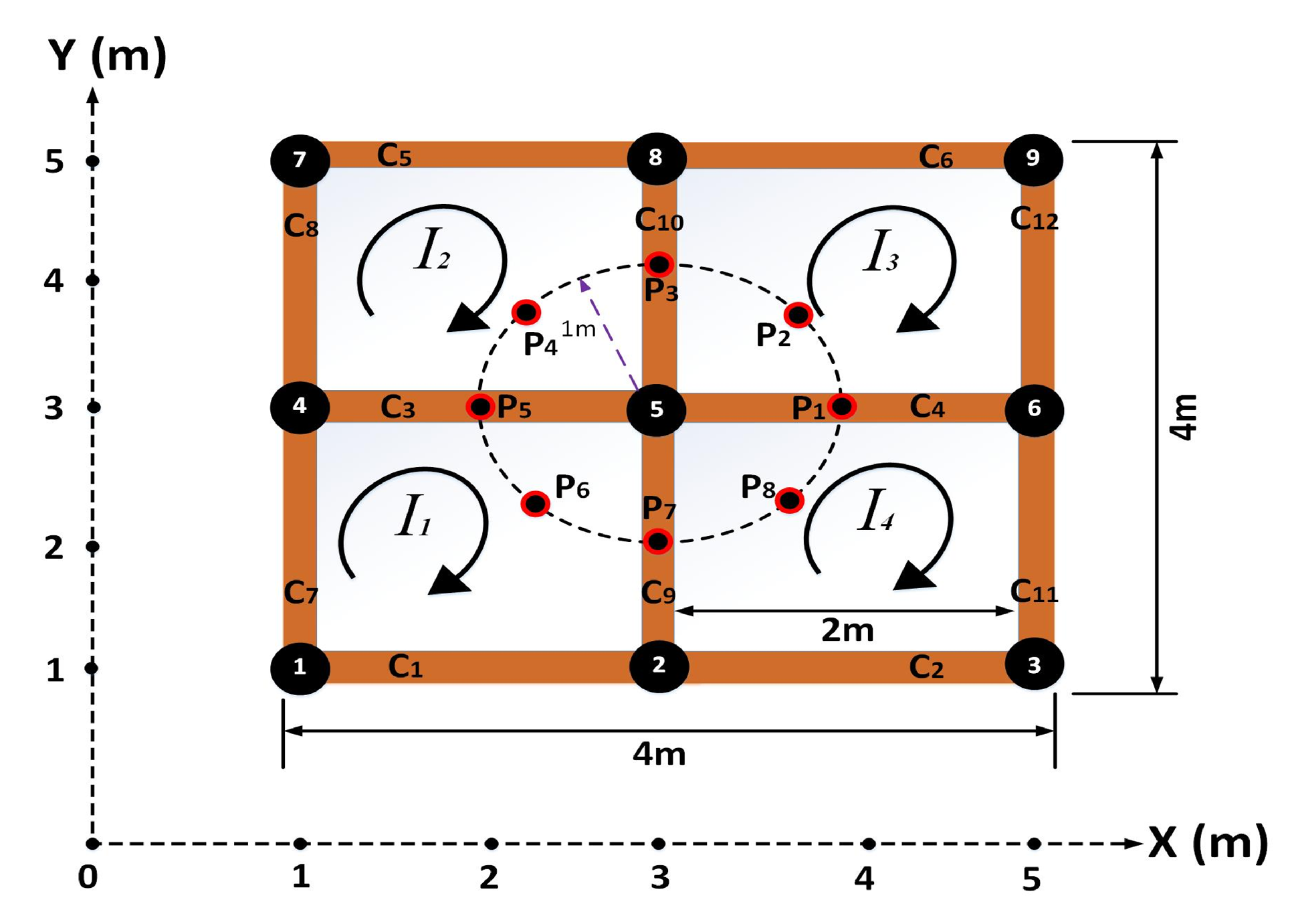
4.1. Simulation Model

The simulation model shown in Figure 5 features a square grid of dimensions 4 m × 4 m. The conductors are labeled $C_1$ to $C_{12}$ and arranged such that the mesh dimensions are 2 m × 2 m. The conductors were cylindrical steel rods of radius 0.01 m and conductivity 4.032 $\times {10}^6$ S/m. The soil considered was homogeneous with electrical resistivity equal to 5 $\mathsf{\Omega }$m. The grounding grid was buried 0.5 m under the Earth’s surface. The transmitter coil of radius 0.15 m was excited with a 16 A pulse current of a trapezoidal wave. The secondary magnetic field was recorded 0.05 m above the surface at the center of the transmitter coil after each 10 $\mathsf{\mu }$s for a total of 100 time samples after the transmitter coil current was turned off. The transmitter coil was moved in a circle of radius 1 m along points $P_1$ to $P_8$ such that the angular displacement between adjacent points was 0.785 rad. The circle was centered at Node 5 acting as pole, which in general must be identified from the position of the vertical conductor. According to IEEE std 80-2013 [5], the length of the grounding grid branches varies from 3 m to 7 m. Therefore, the radius of the circle must be constrained to be between 0 m and 3 m.

Employing the inversion calculation for the secondary magnetic field of Figure 5, the corresponding equivalent resistivity ${\rho }_r$ is plotted in Figure 6. Here, ${\rho }_r$ is high at points $P_1$, $P_3$, $P_5$, and $P_7$, illustrating the presence of conductors $C_4$, $C_{10}$, $C_3$, and $C_9$ at analogous points. For instance, the equivalent resistivity at $P_1$ was high due to the opposite flow of eddy currents $I_3$ and $I_4$ in $C_4$. Keeping in view the rectangular geometry of a typical grounding grid and the characteristics of the polar coordinate system, it is inferred from Figure 6 that the grid was oriented parallel in the plane of the Earth (parallel to the substation boundary). Furthermore, the secondary magnetic field along $P_1$ to $P_8$ is shown in Figure 7. Here, the average value of the magnetic field is plotted against each point. Due to the fact that the magnetic field from a medium is inversely proportional to its resistivity, Figure 7 shows an inverse relation with Figure 6. Therefore, $\overline{H_z}$ was low at $P_1$, $P_3$, $P_5$, and $P_7$, confirming $C_4$, $C_{10}$, $C_3$, and $C_9$.

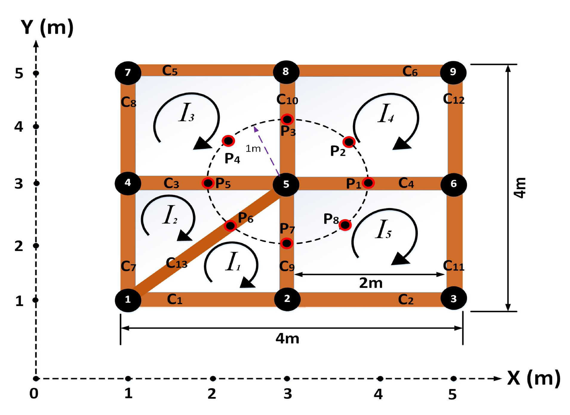
4.2. Grounding Grid with a Diagonal Branch

Grounding grids exist in different configurations depending on the substation layout. A diagonal branch often exits in grounding grids. To check the feasibility of the proposed method for the orientation detection of the grounding grid with a diagonal branch, conductor $C_{13}$ was added to Figure 5. The model with a diagonal branch is shown in Figure 8. $C_{13}$ connected Nodes 1 and 5. TEM was applied by moving the transmitter-receiver pair in a circle from $P_1$ to $P_8$, and the result of equivalent resistivity ${\rho }_r$ is shown in Figure 9. This time, ${\rho }_r$ was high at $P_6$ as eddy currents $I_1$ and $I_2$ opposed each other in $C_{13}$, validating the presence of diagonal conductor $C_{13}$. Contrarily, ${\rho }_r$ at $P_5$ and $P_7$ decreased although conductors $C_5$ and $C_7$ existed beneath them. This was due to unequal magnetic coupling as the mesh size had changed due to the presence of diagonal conductor $C_{13}$. Moreover, the average magnetic field $\overline{H_z}$ graph related to Figure 8 is demonstrated in Figure 10. Diagonal conductor $C_{13}$ was represented by low $\overline{H_z}$ at $P_6$.

4.3. Grounding Grid with Unequal Mesh Spacing

Demonstrating the feasibility of TEM for orientation detection of an unequally spaced grounding grid, Figure 11 is taken into account. In this figure, conductors are labeled $C_1$ to $C_{12}$ and nodes 1 to 9. The dimensions of meshes $M_1$ and $M_2$ were 2.5 m × 2 m, and those of $M_3$ and $M_4$ were 1.5 m × 2 m. Consider Node 5 as a pole and moving the transmitter coil along the circle from point $P_1$ to $P_8$.

In Figure 11, when the transmitter loop was at measuring point $P_1$ with an angle of $0^{\circ }$ and coordinates (4.5,3), currents $I_3$ and $I_4$ flowed in conductor $C_4$ in the opposite direction and canceled each other out. Thus, the current was less and so was the recorded magnetic field at measuring point $P_1$. At points $P_2$ and $P_8$ with angles ${45}^{\circ }$ and ${315}^{\circ }$, respectively, the downward electromagnetic signal coupled extensively with mesh $M_4$ and $M_3$, thus inducing large eddy currents in the meshes. The recorded magnetic field at measuring points $P_2$ and $P_8$ was almost equal and higher than at measuring point $P_1$. Furthermore, when the transmitter loop was at measuring point $P_3$ with an angle of ${90}^{\circ }$, currents $I_3$ and $I_2$ flowed in conductor $C_{10}$ with an unequal magnitude and did not cancel each other completely. This was because of unequal magnetic coupling in meshes $M_4$ and $M_2$. Thus, the recorded magnetic field at measuring point $P_3$ was less than at point $P_2$, but higher than at point $P_4$. Similarly, the recorded magnetic field at measuring point $P_7$ was less than at point $P_8$, but higher than at point $P_6$.

Figure 12 and

Table 1. Recorded magnetic field based on TEM.

Measuring Point	Average Magnetic Field Intensity (A/m)
	Equal Mesh Spacing	Equal Mesh Spacing and Diagonal Branch	Unequal Mesh Spacing
$P_1$	147.0995	264.8785	274.8785
$P_2$	313.9748	340.748	330.748
$P_3$	114.8244	280.854	114.8244
$P_4$	343.3893	313.9748	90.345
$P_5$	114.8244	313.9748	276.74
$P_6$	343.3893	200.051	75.632
$P_7$	114.2897	313.9748	114.8244
$P_8$	313.9748	313.9748	330.748

illustrate that due to weak magnetic coupling, the recorded magnetic field at measuring points $P_4$ and $P_6$ was almost equal and smaller than at measuring points $P_2$ and $P_8$. Thus, the size of grounding grid meshes $M_1$ and $M_2$ was greater than the size of meshes $M_3$ and $M_4$.

Figure 13 displays the distribution of equivalent resistivity ${\rho }_r$ calculated against the circle perimeter in Figure 11. At point $P_1$, ${\rho }_r$ was high since currents $I_3$ and $I_4$ flowed in conductor $C_4$ in the opposite direction. Thus, the current was less, and the equivalent resistivity ${\rho }_r$ was high. As depicted in

Table 2. Equivalent resistivity calculated based on TEM.

Measuring Point	Average Equivalent Resistivity ($\mathbf{\Omega }$m)
	Equal Mesh spacing	Equal Mesh Spacing and Diagonal Branch	Unequal Mesh Spacing
$P_1$	0.2889	0.2976	0.2916
$P_2$	0.2752	0.2736	0.2758
$P_3$	0.2889	0.2911	0.2889
$P_4$	0.2752	0.2752	0.2933
$P_5$	0.2944	0.2752	0.2900
$P_6$	0.2752	0.2982	0.2944
$P_7$	0.2889	0.2752	0.2889
$P_8$	0.2752	0.2752	0.2758

, ${\rho }_r$ at points $P_2$ and $P_8$ in Figure 11 was low as compared to Figure 5. This was due to the small size of meshes $M_4$ and $M_3$ and, therefore, the strong magnetic coupling in these meshes. On the contrary, ${\rho }_r$ was high at $P_4$ and $P_6$ due to the large size of meshes $M_1$ and $M_2$ and, therefore, the weak magnetic coupling. When the transmitter loop was at measuring point $P_3$ with an angle of ${90}^{\circ }$, currents $I_2$ and $I_3$ flowed in conductor $C_{10}$ with unequal magnitude and did not cancel each other. Thus, the calculated equivalent resistivity ${\rho }_r$ at measuring point $P_3$ was higher than at point $P_2$, but smaller than at point $P_4$. Similarly, ${\rho }_r$ at measuring point $P_7$ was higher than at point $P_8$, but smaller than at point $P_6$.

Graphs of the equivalent resistivity ${\rho }_r$ and average magnetic field intensity $\overline{H_z}$ illustrated the presence of conductors $C_3$ and $C_4$ along the x-axis and conductors $C_9$ and $C_{10}$ along the y-axis. It was deduced that the grounding grid was oriented parallel to the plane of the Earth.

5. Conclusions and Future Work

Grounding grid drawings are often lost and mishandled, altering the status of the grid from known to unknown. In this paper, a new method to measure the orientation of the grounding grid was presented. The method was not only independent of the current injection that brought the disturbing inhomogeneity of the surface magnetic flux density, but also did not enhance the effect of the surrounding EME. The transmitter-receiver pair of the TEM system was moved along a circle above the surface such that the vertical conductor acted as the pole of the circle. According to the mesh spacing of the grounding grid between 3 m to 7 m, the radius of the circle was constrained between 0 m to 3 m. Once the equivalent resistivity ${\rho }_r$ was determined from the secondary magnetic field $H_z$, high ${\rho }_r$ and low $\overline{H_z}$ at a point on the circle laid the basis for orientation detection of the grounding grid. Moreover, the proposed method was also investigated for complex mesh configurations including the presence of a diagonal branch and an unequally spaced mesh configuration. As an application, the paper used TEM to measure the orientation of the grounding grid. Simulation results showed that the diagnosis was feasible.

There is a great need for further research to detect grounding grid orientation. This includes a grounding grid with an unequal mesh spacing and a diagonal branch. Furthermore, the depth of the grounding grid must also be considered in future research because it is critical for fault diagnosis.

References

1. Aamir, Q.; Wilayat, K.; Syed, R.N.; Farooq, A.O. Non-destructive depth detection approach for substation grounding grids based on magnetostatics. IET Electron. Lett. 2019, 55, 1121–1123. [Google Scholar] [CrossRef]
2. Gouda, O.E.; Dessouky, S.S.; Kalas, A.E.; Hamdy, M.A. Current distribution in grounding grid conductors with and without vertical rods buried in two-layer soil model. IEEJ Trans. Electr. Electron. Eng. 2018, 13, 1276–1284. [Google Scholar] [CrossRef]
3. Bo, Z.; Wu, J.; He, J.; Zeng, R. Analysis of transient performance of grounding system considering soil ionization by time domain method. IEEE Trans. Magn. 2013, 49, 1837–1840. [Google Scholar] [CrossRef]
4. Hideki, M. Electromagnetic transient response of buried bare wire and ground grid. IEEE Trans. Power Deliv. 2007, 22, 1673–1679. [Google Scholar] [CrossRef]
5. IEEE Std 80-2013 (Revision of IEEE Std 80-2000/Incorporates IEEE Std 80-2013/Cor 1-2015). IEEE Guide for Safety in AC Substation Grounding; IEEE: Piscataway, NJ, USA, 2015.
6. El-Refaie El-Sayed, M.; Elmasry, S.E.; Elrahman MKAbd Abdo, M.H. Achievement of the best design for unequally spaced grounding grids. Ain Shams Eng. J. 2018, 6, 171–179. [Google Scholar] [CrossRef] [Green Version]
7. Ferrante, N. A new evolutionary method for designing grounding grids by touch voltage control. In Proceedings of the IEEE International Symposium on Industrial Electronics, Ajaccio, France, 4–7 May 2004; Volume 2, pp. 1501–1505. [Google Scholar] [CrossRef]
8. Farkoush, S.G.; Wadood, A.; Khurshaid, T.; Kim, C.-H.; Irfan, M.; Rhee, S.-B. Reducing the Effect of Lightning on Step and Touch Voltages in a Grounding Grid Using a Nature-Inspired Genetic Algorithm With ATP-EMTP. IEEE Access 2019, 7, 81903–81910. [Google Scholar] [CrossRef]
9. Farkoush, S.G.; Khurshaid, T.; Wadood, A.; Kim, C.-H.; Kharal, K.H.; Kim, K.-H.; Cho, N.; Rhee, S.-B. Investigation and optimization of grounding grid based on lightning response by using ATP-EMTP and genetic algorithm. Complexity 2018, 2018, 8261413. [Google Scholar] [CrossRef]
10. Aamir, Q.; Muhammad, U.; Fan, Y.; Muhammad, U.; Zeeshan, K. Derivative Method Based Orientation Detection of Substation Grounding Grid. Energies 2018, 11, 1873. [Google Scholar] [CrossRef] [Green Version]
11. Li, X.; Yang, F.; Ming, J.; Jadoon, A.; Han, S. Imaging the Corrosion in Grounding Grid Branch with Inner-Source Electrical Impedance Tomography. Energies 2018, 11, 1739. [Google Scholar] [CrossRef] [Green Version]
12. Yuan, J.; Yang, H.; Zhang, L.; Cui, X.; Ma, X. Simulation of substation grounding grids with unequal-potential. IEEE Trans. Magn. 2000, 36, 1468–1471. [Google Scholar] [CrossRef]
13. Yang, F.; Wang, Y.; Dong, M.; Kou, X.; Yao, D.; Li, X.; Gao, B.; Ullah, I. A Cycle Voltage Measurement Method and Application in Grounding Grids Fault Location. Energies 2017, 10, 1929. [Google Scholar] [CrossRef] [Green Version]
14. Liu, K.; Yang, F.; Wang, X.; Gao, B.; Kou, X.; Dong, M.; Ammad, J. A novel resistance network node potential measurement method and application in grounding grids corrosion diagnosis. Prog. Electromagn. Res. M 2016, 52, 9–20. [Google Scholar] [CrossRef] [Green Version]
15. Liu, Y.; Cui, X.; Zhao, Z. A magnetic detecting and evaluation method of substations grounding grids with break and corrosion. Front. Electr. Electron. Eng. China 2010, 5, 501–504. [Google Scholar] [CrossRef]
16. Yu, C.; Fu, Z.; Wang, Q.; Tai, H.M.; Qin, S. A novel method for fault diagnosis of grounding grids. IEEE Trans. Ind. Appl. 2015, 51, 5182–5188. [Google Scholar] [CrossRef]
17. Aamir, Q.; Nadir, S.; Zeeshan, K.; Zahoor, U.; Farooq, A.O. Breakpoint Diagnosis of Substation Grounding Grid Using Derivative Method. Prog. Electromagn. Res. M 2017, 57, 73–80. [Google Scholar] [CrossRef] [Green Version]
18. Dawalibi, F. Electromagnetic fields generated by overhead and buried short conductors, Part 2—Ground networks. IEEE Trans. Power Deliv. 1986, 1, 112–119. [Google Scholar] [CrossRef]
19. Zhang, X.-L.; Zhao, X.-H.; Wang, Y.-G.; Mo, N. Development of an electrochemical in situ detection sensor for grounding grid corrosion. Corrosion 2010, 66, 076001. [Google Scholar] [CrossRef]
20. Yu, C.; Fu, Z.; Hou, X.; Tai, H.M.; Su, X. Break-point diagnosis of grounding grids using transient electromagnetic apparent resistivity imaging. IEEE Trans. Power Deliv. 2015, 30, 2485–2491. [Google Scholar] [CrossRef]
21. Li, C.; He, W.; Yao, D.; Yang, F.; Kou, X.; Wang, X. Topological measurement and characterization of substation grounding grids based on derivative method. Int. J. Electr. Power Energy Syst. 2014, 63, 158–164. [Google Scholar] [CrossRef]
22. Aamir, Q.; Fan, Y.; Wei, H.; Ammad, J.; Muhammad, Z.K.; Xu, N. Topology measurement of substation’s grounding grid by using electromagnetic and derivative method. Prog. Electromagn. Res. B 2016, 67, 71–90. [Google Scholar] [CrossRef] [Green Version]
23. Yu, C.; Fu, Z.; Wu, G.; Zhou, L.; Zhu, X.; Bao, M. Configuration detection of substation grounding grid using transient electromagnetic method. IEEE Trans. Ind. Electron. 2017, 64, 6475–6483. [Google Scholar] [CrossRef]
24. Fu, Z.; Song, S.; Wang, X.; Li, J.; Tai, H.M. Imaging the topology of grounding grids based on wavelet edge detection. IEEE Trans. Magn. 2018, 54, 1–8. [Google Scholar] [CrossRef]
25. Liu, K.; Yang, F.; Zhang, S.; Zhu, L.; Hu, J.; Wang, X.; Irfan, U. Research on Grounding Grids Imaging Reconstruction Based on Magnetic Detection Electrical Impedance Tomography. IEEE Trans. Magn. 2018, 54, 1–4. [Google Scholar] [CrossRef]
26. Qamar, A.; Yang, F.; Xu, N.; Syed, A.S. Solution to the inverse problem regarding the location of substations grounding grid by using the derivative method. Int. J. Appl. Electromagn. Mech. 2018, 56, 549–558. [Google Scholar] [CrossRef]
27. Mohamed, M.; Gad, E.-Q.; Usama, M.; Abeer, E.-K.; Jun, M.; Naseer, A.-A. Integrated geoelectrical survey for groundwater and shallow subsurface evaluation: Case study at siliyin spring, el-fayoum, egypt. Int. J. Earth Sci. 2010, 99, 1427–1436. [Google Scholar]
28. Xue, G.; Yan, Y.; Li, X.; Di, Q. Transient electromagnetic s-inversion in tunnel prediction. Geophys. Res. Lett. 2007, 34. [Google Scholar] [CrossRef]
29. Adel, K.M.; Maxwell, A.M.; Sergio, L.F. Deep structure of the northeastern margin of the parnaiba basin, brazil, from magnetotelluric imaging. Geophys. Prospect. 2008, 50, 589–602. [Google Scholar] [CrossRef]
30. Yu, C.; Fu, Z.; Zhang, H.; Tai, H.M.; Zhu, X. Transient process and optimal design of receiver coil for small-loop transient electromagnetics. Geophys. Prospect. 2014, 62, 377–384. [Google Scholar] [CrossRef]
31. Misac, N.N. Quasi-static transient response of a conducting half-spacean approximate representation. Geophysics 1979, 44, 1700–1705. [Google Scholar] [CrossRef]
32. Stanley, H.W.; Gerald, W.H.; Misac, N. Electromagnetic theory for geophysical applications. Electromagn. Methods Appl. Geophys. 1988, 1, 131–311. [Google Scholar] [CrossRef]
Figure 1. Grounding grid and its characteristics.
Applsci 09 05270 g001
Figure 2. Grounding grid orientation with respect to the substation boundary. (a) Grounding grid oriented parallel along the substation boundary. (b) Grounding grid with non-parallel orientation along the substation boundary.
Applsci 09 05270 g002
Figure 3. Influence of the surrounding electromagnetic environment (EME) on the derivative method. (a) Surface magnetic flux density B z pertaining to the grounding grid in [26]. (b) Surrounding EME. (c) Mixed signal M z of magnetic flux density B z and the surrounding EME. (d) Derivative of mixed signal M z . This signal contains fake peaks due to the presence of EME, which causes the identification of true peaks to be impossible.
Applsci 09 05270 g003
Figure 4. A typical transient electromagnetic method (TEM) system probing the underground grid. The primary magnetic field due to the transmitter coil interacts with the grid buried in the soil and induces eddy currents. Induced eddy currents produce a secondary magnetic field that travels upward to the Earth’s surface and collected by the receiver coil placed in the center of the transmitter coil.
Applsci 09 05270 g004
Figure 5. Simulation model featuring the square grounding grid of dimensions 4 m × 4 m and mesh spacing 2 m. Conductors are labeled C 1 to C 12 and nodes 1 to 9. I 1 to I 4 are the induced eddy currents whose direction of flow is indicated by arrows. The TEM system is moved 0.05 m above the surface along circle of radius 1 m from point P 1 to P 8 .
Applsci 09 05270 g005
Figure 6. Equivalent resistivity ρ r along the circle from P 1 to P 8 . High ρ r at P 1 , P 3 , P 5 , and P 7 corresponds to the presence of conductors C 4 , C 10 , C 3 , and C 9 . C 4 at 0 rad, C 10 at 1.57 rad, C 3 at 3.14 rad, and C 9 at 4.71 rad along the circle showed the parallel orientation of the grid in the plane.
Applsci 09 05270 g006
Figure 7. Average magnetic field intensity H z ¯ along the circle from P 1 to P 8 . H z ¯ is low at P 1 , P 3 , P 5 , and P 7 , confirming the presence of C 4 , C 10 , C 3 and C 9 , and the parallel orientation of the grid in the plane of the Earth.
Applsci 09 05270 g007
Figure 8. Grounding grid with diagonal conductor C 13 . C 13 connects Nodes 1 and 5 while carrying I 1 I 2 .
Applsci 09 05270 g008
Figure 9. Equivalent resistivity ρ r of Figure 8. High ρ r at P 6 validates the presence of diagonal conductor C 13 . Unequal magnetic coupling due to an unequal mesh size results in low ρ r at P 5 and P 7 .
Applsci 09 05270 g009
Figure 10. Average magnetic field intensity H z ¯ along P 1 to P 8 related to Figure 8. Here, diagonal conductor C 13 is indicated by low H z ¯ at P 6 .
Applsci 09 05270 g010
Figure 11. Grounding grid with an unequal mesh configuration. The dimensions of meshes M 1 and M 2 are 2.5 m × 2 m and M 3 and M 4 are 1.5 m × 2 m.
Applsci 09 05270 g011
Figure 12. Average magnetic field intensity H z ¯ along P 1 to P 8 related to Figure 11. The large size of meshes M 1 and M 2 results in weak magnetic coupling, and therefore, H z ¯ at P 4 and P 6 is less than H z ¯ at P 2 and P 8 .
Applsci 09 05270 g012
Figure 13. Equivalent resistivity ρ r related to Figure 11. The large size of meshes M 1 and M 2 results in weak magnetic coupling and, therefore, ρ r at P 4 and P 6 is higher than ρ r at P 2 and P 8 .
Applsci 09 05270 g013