Simulation of Turbulent Mixing Effects on Essential NO_x–O₃–Hydrocarbon Photochemistry in Convective Boundary Layer

Featured Application

Turbulent Kinetics Model (TKM) expresses nonlinear kinetics and dynamics of chemicals on essential photochemistry in heterogeneous systems with an assumption of a photostationary steady state.

Abstract

The turbulence kinetics model (TKM) describes an overall reaction rate for microscopic mass transfer phenomenon expressed as separation intensity, I_s, in a turbulent reacting flow. This study examines the effects of turbulent mixing in the convective boundary layer (CBL) on essential NOx–O₃–Hydrocarbon photochemistry containing sources of NO and a surrogate reactive hydrocarbon. The modeling approach applies for all species except OH with an assumption of a photostationary steady state. The TKM results reveal principal findings as follows: (1) effects of turbulence on reaction rates lead to significant segregations throughout most of the CBL in reaction pairs NO + O₃, RH + OH and NO + HO₂; (2) segregations permit significantly higher concentrations of NO and RH to build up and endure in the CBL than would occur for a non-turbulent atmosphere; (3) turbulent segregation influences limit and shift the ranges of NO and O₃ concentrations compared to the non-turbulent case; (4) while there are differences between the TKM results and those for a published Large Eddy simulation (LES) of the same chemical system, there are also strong similarities. Therefore, a future study remains to compare model results to observations if and when appropriately time-resolved measurements of reacting species are obtained.

1. Introduction

Natural and environmental engineering systems are considered to be homogeneous systems in which the distribution of matter in the system is neglected at microscopic molecular scale movements and is mainly influenced by macroscopic physical migration phenomena, which affect the reaction energy and rate of reaction. In the homogeneous system, the conversion rate of the chemical is controlled either chemically or kinetically. Generally, it is very complicated to calculate the nonlinear chemical reaction rate in the heterogeneous system, so it tends to be ignored or simplified when assuming the homogeneous system [1]. However, the interaction between two molecules where an actual reaction takes place in a real system is a heterogeneous system in which small microscopic molecular scale turbulent migration phenomena are considered to be important [1]. The asymmetric mixing process strongly controls the chemical reaction rate when the timescale of the chemical reaction is of the same order or faster than the turbulent timescale [1,2,3,4,5,6,7,8]. The chemical reaction rate requires intimate mixing of the species at the molecular-scale (microscale), while dispersion is effected primarily by large-scale turbulent eddies with a nonlinear cascade process resulting in micro-mixing [8].

The largest mixing scale in the turbulent reacting flow is represented by the turbulent Damköhler (D_t) (or non-dimensional reaction rate), which is a ratio of the turbulent time scale (τ_t) to chemical time scale (τ_ch). The D_t affects the segregation between the species in the asymmetric mixing process related to the chemical reaction [9]. Especially, the segregation of the species represents the influence of incomplete mixing on the chemical reaction rate when the chemical reaction time scale is similar to the turbulent time scale ($\left|D_t\right|\ge 1$). If the chemical reaction is extremely slow relative to the mixing processes ($\left|D_t\right|\ll 1$), the reactants become effectively well mixed. Also, the reacting species remain segregated in the case of very fast chemical reactions relative to mixing ($\left|D_t\right|\gg 1$).

In a heterogeneous system, it is limited to the overall reaction rate due to the microscopic mass transfer phenomenon and can be expressed as the separation intensity, I_s [3,4,5,7]. The intensity of segregation I_s clearly depends on the turbulent Damköhler number and it can be related to the concentration fluctuation $\overline{c_A^{\prime }{c}_B^{\prime }}$ and the mean concentrations${\overline{C}}_A$ and ${\overline{C}}_B$ of the reactive species A and B; $I_s=\overline{c_A^{\prime }{c}_B^{\prime }}/\left({\overline{C}}_A{\overline{C}}_B\right)$. The concentration fluctuation needs to be well specified because the turbulent mixing effect on the chemical reaction rate can be measured by the concentration fluctuation. The effective (nonlinear) reaction rate is varied with the concentration covariance (fluctuation) that is a measure of segregation between two reactants, is directly related to the micromixing phenomena, and then is lowered or enhanced depending on whether the covariance is negative (non-premixed reactants) or positive (premixed reactants). Thus, the effective reaction rates, R_e, in terms of the covariance can be rewritten in terms of the intensity of segregation I_s.

$$R_e=-k_f\left({\overline{C}}_A{\overline{C}}_B+\overline{c_A^{\prime }{c}_B^{\prime }}\right)$$

$$R_e=-k_f\left(1+I_s\right){\overline{C}}_A{\overline{C}}_B$$

The turbulent mixing effect on the chemical reaction rate can expressed as a function of the intensity of segregation I_s (I_s = −1 for the complete segregation between the species, I_s = 0 for the perfectly mixed species by the turbulence, and I_s > 0 or I_s < 0 for the enhanced or lowered reaction rate compared to the perfectly mixed case).

The reaction of NO and O₃ in the atmosphere should consider the effect of turbulence with D_t ≥ 1 when the intensity of segregation is always negative in the situation where both species are introduced at opposite boundaries [10]. Large regional ozone studies have been carried out in the San Joaquin Valley (central California) [11], Southeastern United States [12,13,14,15], Lake Michigan [16], Northeastern United States [17,18], United States [19,20], eastern North America [21], Russia [22], and Australia [23]. In those areas, maximum ozone concentrations during the summer exceeded the O₃ national ambient air quality standard (NAAQS) of 70 ppb finalized by the USEPA in 2015. Ozone studies have led to the recognition that realistic representations of turbulent mixing processes are very important for air quality simulation.

The effects of incomplete mixing on the chemical reaction between two species such as NO and O₃ are potentially very important when the time scale of the chemical reaction is of the same order or faster than the turbulent time scale [3,4,5,6,7,8,10]. A 1-D Turbulent Kinetics Model (TKM) [10] is applied to study the NO_x–O₃ cycle as a representative reaction system whose reaction rates are affected by turbulent mixing in the convective boundary layer (CBL). The TKM chemical kinetics expression is modified by a term containing the covariance of the reactant concentrations in order to account for the effects of turbulence. Other studies have extended the scope to a more complex chemistry mechanism containing a wide range of chemical time scales [24,25,26]. The vertical turbulent transport of trace reactive species (the O₃–NO–NO₂ triad) in the CBL during daytime has been used in the Second-Order Model for Conserved and Reactive Unsteady Scalars (SOMCRUS)[24]. SOMSCRUS [27,28] is run to investigate reactive species in the CBL and to obtain continuous equilibrium profiles of turbulent fluxes and mean concentrations of reactive scalars (the O₃–NO–NO₂ triad) in a steady-state CBL without shear [29]. Also, SOMCRUS is used to calculate time-varying continuous profiles of mean concentrations and vertical turbulent fluxes, variances and covariances of both passive and reactive scalars (the O₃–NO–NO₂ triad) [24]. A system in a simulation with a 1-D coupled diffusion and chemistry model applies a second-order closure scheme in the neutral Atmospheric Boundary Layer (ABL) over a remote deciduous forest [26]. However, those studies used the mean reaction rate formulation of the chemical kinetics which neglected the contribution of the covariance term. The turbulent effect on chemical reaction rates has been studied for “essential” daytime photochemistry with hydrocarbons and with various chemical time scales in the CBL by means of a large eddy simulation (LES)[25]. Those results showed that turbulence played a relatively modest role in affecting the evolution of the reaction system. The present study has an originality to develop the computational turbulent kinetic model (TKM) for expressing nonlinear kinetics and dynamics of chemicals in heterogeneous systems. For validating TKM applicability, model simulations are run for essential NO_x–O₃–RH photochemistry in a convective boundary layer (CBL). The present study uses the turbulent kinetics model (TKM) [10] and a set of photochemical reactions [25] to simulate the effects of turbulence on the reaction rates and distribution of important species in the CBL. For this purpose, this study compare the TKM results to those of a box model (BM), a conventional kinetics model (CKM) and the LES model [25]. Also, this study aims at providing the results of a sensitivity analysis of the TKM to show the effects of changes in such important parameters as nitric oxide (NO) and hydrocarbon (HC or RH) emission rates, reaction rate constants, dry deposition velocity, exchange velocity, turbulent time scale, and initial concentrations of species.

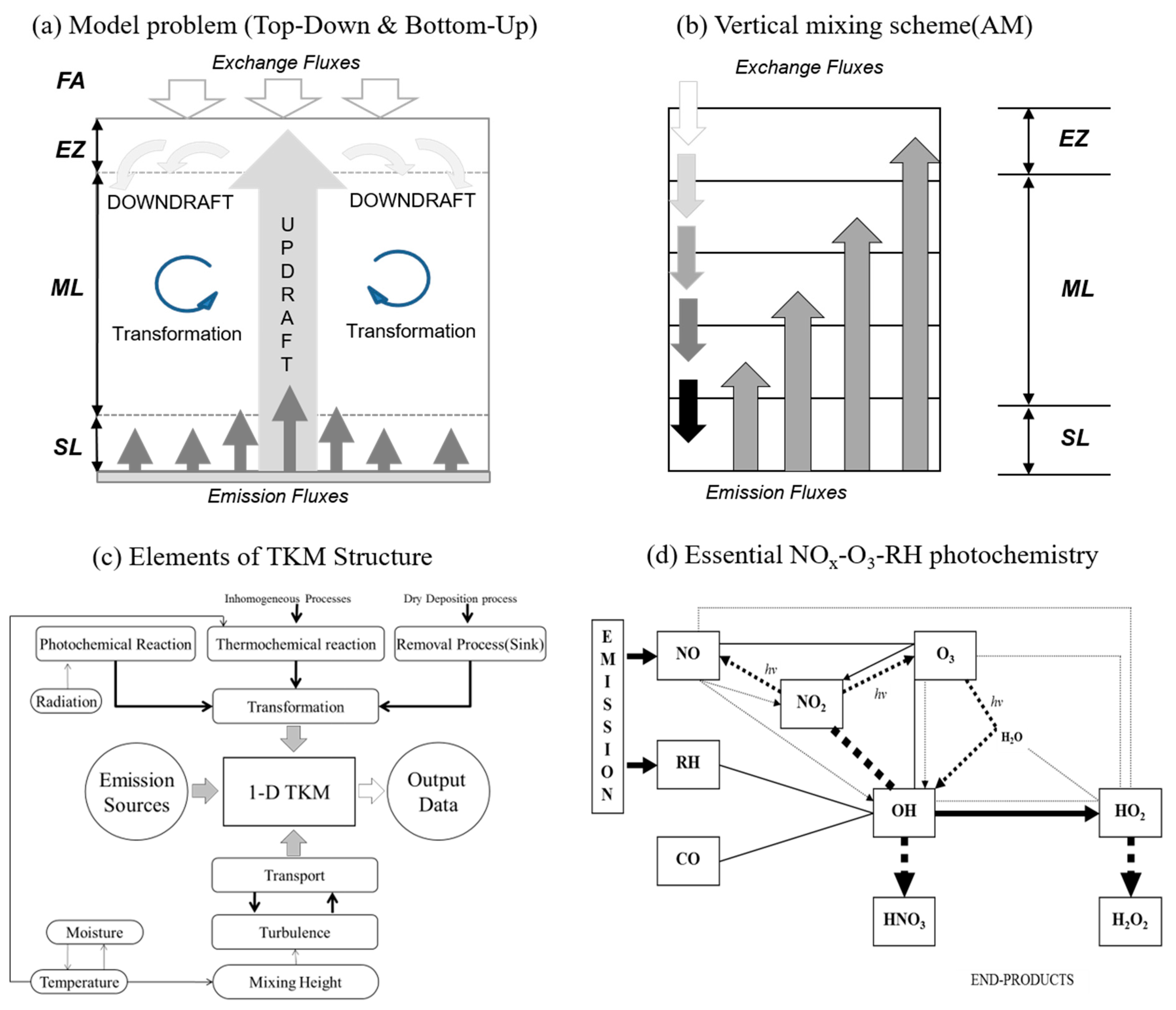
2. Model Description

2.1. Model Reactions

The TKM has been developed in the previous study [10] with the assumption of horizontally homogeneous and vertically heterogeneous CBL in a quasi-steady-state characteristic of a summer cloud-free daytime as shown schematically in Figure 1a for the CBL with coupled chemical kinetics [10]. The TKM includes an asymmetric turbulent transport process to explain the macromixing influence represented by top-down and bottom-up(TDBU) diffusion of two species using the concept of the asymmetric convective model(ACM) [30] presented in Figure 1b. Figure 1c reveals elements of the 1-D TKM structure: The source is expressed by an emission term, a transport process (vertical mixing by turbulence), a transformation process (photochemical reaction, thermal chemical reaction, removal by dry deposition process expressed by a sink term), and output.

In this study, the TKM is applied to the daytime essential NO_x–O₃–RH photochemical system [25] with the reactions listed in

Table 1. The essential photochemical reaction scheme at 298 °K.

Reactions	Reactants	Products	Parameter	Rate Constant at 298 °K
				S90 a	CB-IV c
R1	O3 $\stackrel{{\mathrm{H}}_2\mathrm{O}}{\to }$	2 OH + O2	J1 b	2.7 × 10−6	2.7 × 10−6
R2	NO2 $\stackrel{{\mathrm{O}}_2}{\to }$	NO + O3	J2	8.9 × 10−3	8.9 × 10−3
R3	O3 + NO →	NO2 + O2	k1	4.75 × 10−4	4.49 × 10−4
R4	OH + CO $\stackrel{{\mathrm{O}}_2}{\to }$	HO2 + CO2	k2	6.0 × 10−3	3.18 × 10−3
R5	OH + RH →	HO2 + products	k2 × f	6.0 × 10−3 × f	3.18 × 10−3 × f
R6	HO2 + NO →	OH + NO2	k3	2.1 × 10−1	2.04 × 10−1
R7	HO2 + O3 →	OH + 2 O2	k4	5.0 × 10−5	3.87 × 10−5
R8	2 HO2 →	H2O2 + O2	k5	7.25 × 10−2	4.24 × 10−2
R9	OH + NO2 →	HNO3	k6	2.75 × 10−1	3.59 × 10−1
R10	OH + O3 →	HO2 + O2	k7	1.75 × 10−3	1.68 × 10−3
R11	OH + HO2 →	H2O + O2	k8	2.75	2.75

^a All reaction rate constants are taken from [31]. Photolysis frequencies are given in s⁻¹. Reaction rates are given in ppb⁻¹∙s⁻¹. The factor f that appears in the reaction rate of RH + OH is variable and ranges from 100 to 300. Initially, f is set to 100. A constant Relative humidity (Rh) is assumed as 45%. ^b J₁ is the product of the photolysis frequency for O₃ + hv → O(¹D) + O₂ multiplied by the yield of the reaction O(¹D) +HO₂. Sources: [25]. ^c Reaction rate constants are taken from Carbon-bonding mechanism IV (Harvey, http://airsite.unc.edu/soft/cb4/cb4main.html) [32] except those for R₁, R₂, and R₁₁.

and Figure 1d. The species in the system are ozone (O₃), the oxides of nitrogen (NO, NO₂ and HNO₃), the oxides of hydrogen (OH, HO₂, H₂O, and H₂O₂), and a generic hydrocarbon (RH). All but HNO₃ and H₂O₂ have lifetimes similar to or shorter than the turbulent time scale (667 s in this paper). A constant CO concentration represents all the carbon species that have long lifetimes compared to the turbulent time scale (e.g., methane and CO). Water vapor is considered to be present at a constant concentration [25]. The product species HNO₃ and H₂O₂ are not reactive and their concentrations increase with time in the model simulations, which assume they are not removed by dry deposition. Although this mechanism is oversimplified in its representation of atmospheric chemistry, it contains most of the key features included in more detailed mechanisms. Thus, this chemical mechanism can be used to illustrate the qualitative features of the general hydrocarbon–NO_x–O₃ chemistry in the troposphere. The mechanism consists of the reactions listed in Table 1 and Figure 1d.

For the present purposes, this study considers that the chemical processes start with the photolysis of O₃ and NO₂ (R₂). These and the reaction between NO and O₃ are responsible for maintaining much of the O₃ concentrations (see Reference [10]). However, the long-term behavior of NO (and thus of O₃) depends upon the more complex chemistry, the essence of which is embodied in reactions R₁–R₁₁ listed in Table 1. This set of reactions and terminology are referred to as the essential daytime photochemistry in Reference [25]. The key to understanding the chemistry is the centrally important OH radical. The OH radical via R₄ and R₅ oxidizes hydrocarbons (CO and RH). The HO₂ radicals react with NO to regenerate OH and complete the cycle (R₆). The photolysis of O₃ generates O(¹D) which subsequently reacts with water to form OH radicals. Both steps are represented in the essential chemistry mechanism by the single reaction R₁. Termination of the reaction chain occurs via R₉, R₈ and R₁₁. The concentration of H₂O is assumed to be constant since it is determined mainly by the physical hydrologic and meteorological conditions.

Constant CO concentration represents CO itself and all the hydrocarbons that have long lives compared to the turbulent timescale (e.g., methane). The rate constant for the reaction of CO with OH (R₄) is taken to be that for CO alone. For the reaction of RH with OH (R₅), the rate constant is expressed as the product of the constant for the CO reaction with OH and a parameter f. Also, the chemistry of the reaction between RH and OH is simplified by assuming it produces HO₂ as the only product of importance to the chemical scheme. Pseudo-Steady-State Approximation in the development of turbulence (PSSAt) and Photostationary Steady-State Approximation in the chemical reaction (PSSAc) are assumed for OH and HO₂ radicals, which have very short lifetimes. Thus, the production and destruction of OH is determined by the longer-lived species and its concentration can be calculated from (see [25]):

$${\left({\overline{C}}_{OH}\right)}_{SS}=\frac{2j_1{\overline{C}}_{O_3}+k_3{\overline{C}}_{H{O}_2}{\overline{C}}_{NO}+k_4{\overline{C}}_{H{O}_2}{\overline{C}}_{O_3}}{k_2\left({\overline{C}}_{CO}+f{\overline{C}}_{RH}\right)+k_6{\overline{C}}_{N{O}_2}+k_7{\overline{C}}_{O_3}+k_8{\overline{C}}_{H{O}_2}}.$$

(1)

2.2. Model Equations

The TKM describes the reactions which occur over a substantial range of chemical time scales in a dry CBL with turbulence driven by constant surface heat flux without cumulus convection when the growth of the CBL is ignorable during the afternoon in the summer months as shown in Figure 1a. Previously, the TKM has conducted a simple NO_x–O₃ photochemistry study to quantitatively account for turbulence-induced incomplete mixing of two interacting chemical species [10]. In this study, the NO and O₃ fluxes are not opposite in sign, which means they both have net upward transfers, so they are diluted in the upper CBL due to entrainment of ‘clean air’ from the free troposphere.

Governing equations in the TKM are described using a concentration field splitting method (CSM) for an effective chemical reaction rate [33,34] and a non-local closure asymmetric convective model (ACM) for the vertical mixing scheme [30]. As a computationally simple scheme, as shown in Figure 1b, the ACM provides realistic simulation of vertical mixing in the CBL as mentioned in the Appendix. The effective reaction rate related to the intensity of segregation I_s can be calculated using the concept of the CSM which explains the possible states of mixing of the two species considering the concentration fields (the reactive species and their inert surrogates) in position and time. Based on the CSM considering the binary reaction between A and B, the hypothetical concentrations of inert species A^I and B^I are present in the same position and time with the reactive concentration of the reactive species A and B because the species A^I, B^I, A and B transport in the same convective flow of the CBL. Also, the concept of a local phenomenal extent reaction ξ incorporates both stoichiometry and diffusion effects simultaneously in space and time. To reduce the number of partial differential equations needed to describe the evolution of multimolecular systems in the turbulent (incompletely mixed) field, the stoichiometric relations are combined with the concept of inert surrogate concentrations (see References [10,30,31] for details). Therefore, the mean concentration of the reactive species A and B, ${\overline{C}}_A\mathrm{and}{\overline{C}}_B$, can be calculated using the inert surrogate mean concentration, ${\overline{C}}_A^I\mathrm{and}{\overline{C}}_B^I$, and the phenomenal extent of reaction ξ in space and time ($\overrightarrow{x},t$): ${\overline{C}}_A\left(\overrightarrow{x},t\right)={\overline{C}}_A^I\left(\overrightarrow{x},t\right)-\overline{\xi }\left(\overrightarrow{x},t\right)$ and ${\overline{C}}_B\left(\overrightarrow{x},t\right)={\overline{C}}_B^I\left(\overrightarrow{x},t\right)-\overline{\xi }\left(\overrightarrow{x},t\right)$ for two reactants and ${\overline{C}}_P\left(\overrightarrow{x},t\right)={\overline{C}}_P^I\left(\overrightarrow{x},t\right)+\overline{\xi }\left(\overrightarrow{x},t\right)$ for product P.

The governing equations of variables in the TKM for inert species, for reactive species, and for phenomenal extent of reaction ξ are time-dependent, nonlinear and coupled partial differential equations, which are expressed in a fixed Eulerian framework as given below (see Reference [10] for details):

$$\begin{array}{}\mathrm{(2)}& \left(\frac{\partial \overline{C_i^I}}{\partial t}\right)& =& -\left(\frac{\partial \overline{w^{\prime }{c}_i^I{}^{\prime }}}{\partial z}\right)& +& {\overline{S}}_i\hfill \mathrm{(3)}& (\frac{\partial {\overline{C}}_i}{\partial t})& =& -\left(\frac{\partial \overline{w^{\prime }{c}_i^{\prime }}}{\partial z}\right)& +& \left({\overline{S}}_i+{\overline{R_e}}_c\right)\hfill \mathrm{(3a)}& \left(\frac{\partial {\overline{\xi }}_i}{\partial t}\right)& =& -\left(\frac{\partial \overline{w^{\prime }{\xi }_i^{\prime }}}{\partial z}\right)& +& \left({\overline{S}}_i+{\overline{R_e}}_c\right)\hfill & \mathrm{I}& & \mathrm{II}& & \mathrm{III}\hfill \end{array}$$

where, term I is the local rate of change of the variables, term II is the vertical turbulent flux transport, term III is the source and sink term, and i is the species A and B. The source term in term III is ${\overline{S}}_i=E/\Delta z$, where E(ppb∙m∙s⁻¹) is the emission flux of species A at the surface level Δz, or it is the entrained flux of species B at the top level Δz. The effective reaction rate, $\overline{R_{e_c}}$ (ppb∙s⁻¹) for the sink term in term III is calculated for the mean phenomenal extents of reaction based on the CSM (see Section 2.3 for details). In this study, the mean concentration of reactive species is calculated using the inert surrogate mean concentration ${\overline{C}}_i^I$ and the phenomenal extent of reaction $\overline{\xi }$ instead of using Equation (3): ${\overline{C}}_i={\overline{C}}_i^I-\overline{\xi }$ for reactants and ${\overline{C}}_i={\overline{C}}_i^I+\overline{\xi }$ for products. The governing equations of variables in the TKM are solved by forward finite difference methods (FFDM). For the numerical integration of μ_i and μ_j, $\partial {\mu }_i/\partial t=\left({{\mu }_i|}_{m+1}-{{\mu }_i|}_m\right)/\Delta t$ and $\partial {\mu }_j/\partial t=\left({{\mu }_j|}_{m+1}-{{\mu }_j|}_m\right)/\Delta t$, with the current time step m and the next time step m + 1 and the time difference Δt between m and m + 1.

2.3. Model Approaches

The major governing equations solved in the TKM are the same as those described in the previous study [10]. The symbols and subscripts have, in general, the same meanings, but now the subscript i denotes species NO, O₃, NO₂, RH, HO₂, and OH, and subscript j denotes the partner of species i for chemical reactions detailed in Table 1 (e.g., for NO in a reaction, R₃, i = NO and j = O₃). Similarly, the source, sink and reaction rate terms are formulated to account for surface sources of NO and RH, dry deposition removal of species, entrainment of species from the free troposphere above the CBL, and the reactions listed in Table 1. The overall effective reaction rate (ppbv∙s⁻¹) for species i is

$${\overline{R}}_{e_{c_i}}=\sum R_k$$

(4)

where R_k represents an individual reaction and subscript k denotes reaction number in Table 1 for all reactions of species involving species i. For example, the overall effective reaction rate of the species NO is

$${\overline{R}}_{e_{c_i}}=\sum R_k=R_2-R_3-R_6$$

(5)

The individual reaction R_k between species i and j is expressed in terms of the segregation coefficient $I_{s_{ij}}$ as

$${\overline{R}}_k=-k\left(1+I_{s_{ij}}\right){\overline{C}}_i{\overline{C}}_j\mathrm{or}{\overline{R}}_k=-k\left(1+I_{s_{ij}}\right)\left({\overline{C}}_i^I-{\overline{\xi }}_i\right)\left({\overline{C}}_j^I-{\overline{\xi }}_j\right)$$

(6)

$$I_{s_{ij}}=\left\{\frac{{\phi }_{ij}\left[1+I_{s_{ij}}^I\right]\left[1-\left(1-{\mu }_i\right){\overline{C}}_i^I/{\overline{C}}_i\right]\left[1-\left(1-{\mu }_j\right){\overline{C}}_j^I/{\overline{C}}_j\right]}{{\mu }_i{\mu }_j}\right\}-1$$

(7)

where $I_{s_{ij}}^I$ is the intensity of segregation for inert species $I_{s_{ij}}^I=\left(\overline{c_i^{I^{\prime }}{c}_j^{I^{\prime }}}\right)/\left({\overline{C}}_i^I{\overline{C}}_j^I\right)$; µ_i and µ_j are the mixing parameters ${\mu }_i=\left(1+I_{s_{ij}}^I\right)/\left(1+I_{jj}^I\right)$ with $I_{jj}^I=\overline{{\left(c_j^I{}^{\prime }\right)}^2}/{\left({\overline{C}}_j^I\right)}^2$ and ${\mu }_j=\left(1+I_{s_{ij}}^I\right)/\left(1+I_{ii}^I\right)$ with $I_{ii}^I=\overline{{\left(c_i^I{}^{\prime }\right)}^2}/{\left({\overline{C}}_i^I\right)}^2$; and ${\phi }_{ij}$ is the reaction parameter as below:

$$\begin{array}{ll}\frac{1}{{\phi }_{ij}}\frac{\partial {\phi }_{ij}}{\partial t}=& \frac{2D}{l_d^2}\left[1-\frac{{\mu }_i{\mu }_j}{\left(1+I_{s_{ij}}^I\right)}\right]\\ & -\{\frac{2D}{l_d^2}\left[1-\frac{\left({\overline{C}}_i-\langle 1-{\mu }_i\rangle {\overline{C}}_i^I\right)\left({\overline{C}}_j-\langle 1-{\mu }_j\rangle {\overline{C}}_j^I\right)}{\left(1+I_{s_{ij}}\right){\overline{C}}_i{\overline{C}}_j}\right]\\ & +k\left[\left(1-{\mu }_i\right){\overline{C}}_i^I+\left(1-{\mu }_j\right){\overline{C}}_j^I\right]\}\frac{{\phi }_{ij}\left(1+I_{s_{ij}}^I\right)}{{\mu }_i{\mu }_j}\\ & +\frac{\left({\overline{C}}_i-{\overline{C}}_i^I\right)}{{\mu }_i{\overline{C}}_i^I\left({\overline{C}}_i-{\overline{C}}_i^I+{\mu }_i{\overline{C}}_i^I\right)}\left({\mu }_i\frac{\partial {\overline{C}}_i^I}{\partial t}+{\overline{C}}_i^I\frac{\partial {\mu }_i}{\partial t}\right)\\ & +\frac{\left({\overline{C}}_j-{\overline{C}}_j^I\right)}{{\mu }_j{\overline{C}}_j^I\left({\overline{C}}_j-{\overline{C}}_j^I+{\mu }_j{\overline{C}}_j^I\right)}\left({\mu }_j\frac{\partial {\overline{C}}_j^I}{\partial t}+{\overline{C}}_j^I\frac{\partial {\mu }_j}{\partial t}\right)\end{array}$$

where D is the molecular diffusivity of species i and j [m² s⁻¹](D = D_i = D_j); I_d is the turbulent dissipative scale length [m]; $\overline{{\left(c_i^{I^{\prime }}\right)}^2}$ and $\overline{{\left(c_j^{I^{\prime }}\right)}^2}$ are the concentration variances of inert species i and j; and $\left(\overline{c_i^{I^{\prime }}{c}_j^{I^{\prime }}}\right)$ is the concentration covariance of inert species i and j.

The concentration variance and concentration covariance of inert species i and j are expressed by Equations (8) and (9), respectively.

$$\begin{array}{}\mathrm{(8)}& \left[\frac{\partial \overline{{\left(c_i^{I^{\prime }}\right)}^2}}{\partial t}\right]& =& -\left[\frac{\partial \overline{w^{\prime }{\left(c_i^{I^{\prime }}\right)}^2}}{\partial z}\right]& -\left(2\overline{w^{\prime }{c}_i^{I^{\prime }}}\frac{\partial {\overline{C}}_i^I}{\partial z}\right)& -\left[2D\left(\frac{\partial \overline{c_i^{I^{\prime }}}}{\partial z}\right)\left(\frac{\partial \overline{c_i^{I^{\prime }}}}{\partial z}\right)\right]\mathrm{(9)}& \left[\frac{\partial \overline{\left(c_i^{I^{\prime }}{c}_j^{I^{\prime }}\right)}}{\partial t}\right]& =& -\left[\frac{\partial \overline{w^{\prime }\left(c_i^{I^{\prime }}{c}_j^{I^{\prime }}\right)}}{\partial z}\right]& -\left(\overline{w^{\prime }{c}_j^{I^{\prime }}}\frac{\partial {\overline{C}}_i^I}{\partial z}+\overline{w^{\prime }{c}_i^{I^{\prime }}}\frac{\partial {\overline{C}}_j^I}{\partial z}\right)& -\left[2D\left(\frac{\partial \overline{c_i^{I^{\prime }}}}{\partial z}\right)\left(\frac{\partial \overline{c_j^{I^{\prime }}}}{\partial z}\right)\right]& \mathrm{I}& & \mathrm{II}& \mathrm{III}& \mathrm{IV}\end{array}$$

where, term I is the local rate of change, term II is the vertical turbulent flux transport processes, term III is the mean gradient production processes, and term IV is the molecular dissipation of the mean concentration variance and covariance for inert species i and j and of the mean concentration covariance for reactive species i and j [ppb²∙s⁻¹] (refer to Reference [10] for details).

3. Model Simulation

3.1. Simulation Description

For the TKM simulations, this study adopted the initial and boundary conditions and the parameter values from the Reference [25] for typical conditions of a continental boundary layer during daytime in summer. This study assumed the temperature to be constant at 298 K and the water vapor to have a concentration representing a relative humidity Rh = 45 %.

Table 2. Initial and boundary conditions to simulate TKM based on the essential photochemistry described in Table 1.

Symbol	Value	Unit	Description
Zsfc	0	m	Surface height
Zi	1000	m	Boundary layer height
t*	667	s	Convective time scale
T0	298	ºK	Surface temperature
0	296.88	ºK	Surface potential temperature
P	101,325	Pa	Surface pressure
d (=g/Cp)	0.009764	ºK m−1	Environmental temperature lapse rate
kf	See Table 1 for reaction rate constants
j1	See Table 1 for photolysis rate
w*	1.5	m∙s−1	Convective velocity scale
we	0.01	m∙s−1	Entrainment velocity
ENO	0.1	ppb∙m∙s−1	Typical NO emission flux for an agricultural area at sfc
ERH	1.0	ppb∙m∙s−1	A realistic RH emission flux at surface based on isoprene flux measurements [35]
Edi	we(CiCBL-CiFA)	ppb∙m∙s−1	Downward entrance at entrainment for all species shown in Table 1
kh	64	Non-d	Number of layers in model
t	0.1	s	Time step
tmax	200	min	Simulation run time
z	15.63	m	Non-uniform grid space of model layer
Mu	0.0015	s−1	Upward mixing rate
CNOi(CNOf)	0.138(0.0114)	ppb	Initial NO concentration in CBL (in free atmosphere(FA))
CO3i(CO3f)	68.8(50.0)	ppb	Initial O3 concentration in CBL (in FA)
CNO2i(CNO2f)	0.608(0.0386)	ppb	Initial NO2 concentration in CBL (in FA)
CRHi(CRHf)	3.0(0.0)	ppb	Initial RH concentration in CBL (in FA)
CHO2i(CHO2f)	35.1(33.5)	ppt	Initial HO2 concentration in CBL (in FA)
COHi(COHf)	0.537(0.548)	ppt	Initial OH concentration in CBL (in FA)
Vd_NO	0.0002	m∙s−1	Dry deposition velocity of NO
Vd_O3	0.005	m∙s−1	Dry deposition velocity of O3
Vd_NO2	0.005	m∙s−1	Dry deposition velocity of NO2
Vd_RH	0.001	m∙s−1	Dry deposition velocity of RH
Vd_HO2	0.01	m∙s−1	Dry deposition velocity of HO2
Vd_OH	0.01	m∙s−1	Dry deposition velocity of OH
Vd_HNO3	0.04	m∙s−1	Dry deposition velocity of HNO3
Vd_H2O2	0.01	m∙s−1	Dry deposition velocity of H2O2

lists all of the conditions and assumptions used in the simulations. Homogeneous initial concentrations in the CBL were calculated from the chemical steady state using the Box Model (BM). At the surface, all species are removed according to their respective deposition velocities. The previous study [25] used a value of the dry deposition velocity for O₃ and NO₂ estimated from the study [35] and took arbitrary values for the other species. However, the dry deposition velocity for NO [25] is large (0.2 cm∙s⁻¹) compared to that of other studies [26,36]. Based on the previous studies, this study assumed a value of the deposition velocity for NO of 0.02 cm∙s⁻¹ [26] and the following surface emission fluxes [25]: For NO, 0.1 m∙s⁻¹, and for RH, 1.0 m·s⁻¹. The NO emission flux is typical of an agricultural area and that of RH (all reactive hydrocarbons and intermediates) is based on isoprene flux determinations [37]. The flux at the top of the CBL is calculated using the exchange velocity w_e, which is equal to 0.01 cm∙s⁻¹, and the concentration differences between the top layer of the CBL and the free troposphere (FT); thus, exchange flux = w_e (C_CBL − C_FT). As indicated previously, the end-product species HNO₃ and H₂O₂ are assumed to have zero deposition velocity.

Numerical simulations are carried out for the full governing equations using a forward time finite difference scheme. Concentrations, concentration variances, concentration covariances, fluxes, and the reaction parameters are computed using a grid spacing (64 grid points) distributed uniformly in altitude between the surface and the top of the CBL (Z_i = 1000 m height). A time step of 1.5 s was used for all simulations, which lasted for 200 min in the model domain.

3.2. Comparison Description

Because there are no observational data suitable for validating our model and those of other models mentioned in this paper, this study compares the TKM model results to those of the 3-D LES model [25] and to several simplified model variants, as listed below and described in

Table 3. Description of Models for simulating Model Problems: BMch (Photochemical Box Model with chemistry only), BM (Box Model with chemical and physical processes), CKM (Conventional Kinetics Model with mean reaction rate and ACM), and TKM (Turbulent Kinetics Model with concentration fluctuation using conventional extent of reaction and ACM.

Model	BMch	BM	CKM	TKM
Conditions	All the same conditions described in Table 2 (no emission source in BMch; only depending upon initial concentrations and photochemistry of species)
Deposition term	No	Concentration in BM	Concentration at lowest model layer (surface layer)
Vertical Diffusion term	No	No	Asymmetric Convective Model (ACM): vertical mixing scheme
Chemical Kinetics term: for Irreversible Reaction $A+B\to P$	Mean reaction rate ${{\overline{R}}_m|}_{CKM,BM,BMch}=-k_f\left(\overline{C_A}\right)\left(\overline{C_B}\right)$			Effective reaction rate ${{\overline{R}}_{e_c}|}_{TKM}=-k_f\left({\overline{C}}_A{\overline{C}}_B+\overline{c_A^{\prime }{c}_B^{\prime }}\right)$ Using Concentration Splitting Method (CSM) with segregation coefficient Is,AB in Equation (4) ${{\overline{R}}_{e_c}|}_{TKM}=-k_f\left(1+I_{s_{AB}}\right)\left({\overline{C}}_A\right)\left({\overline{C}}_B\right)$

.

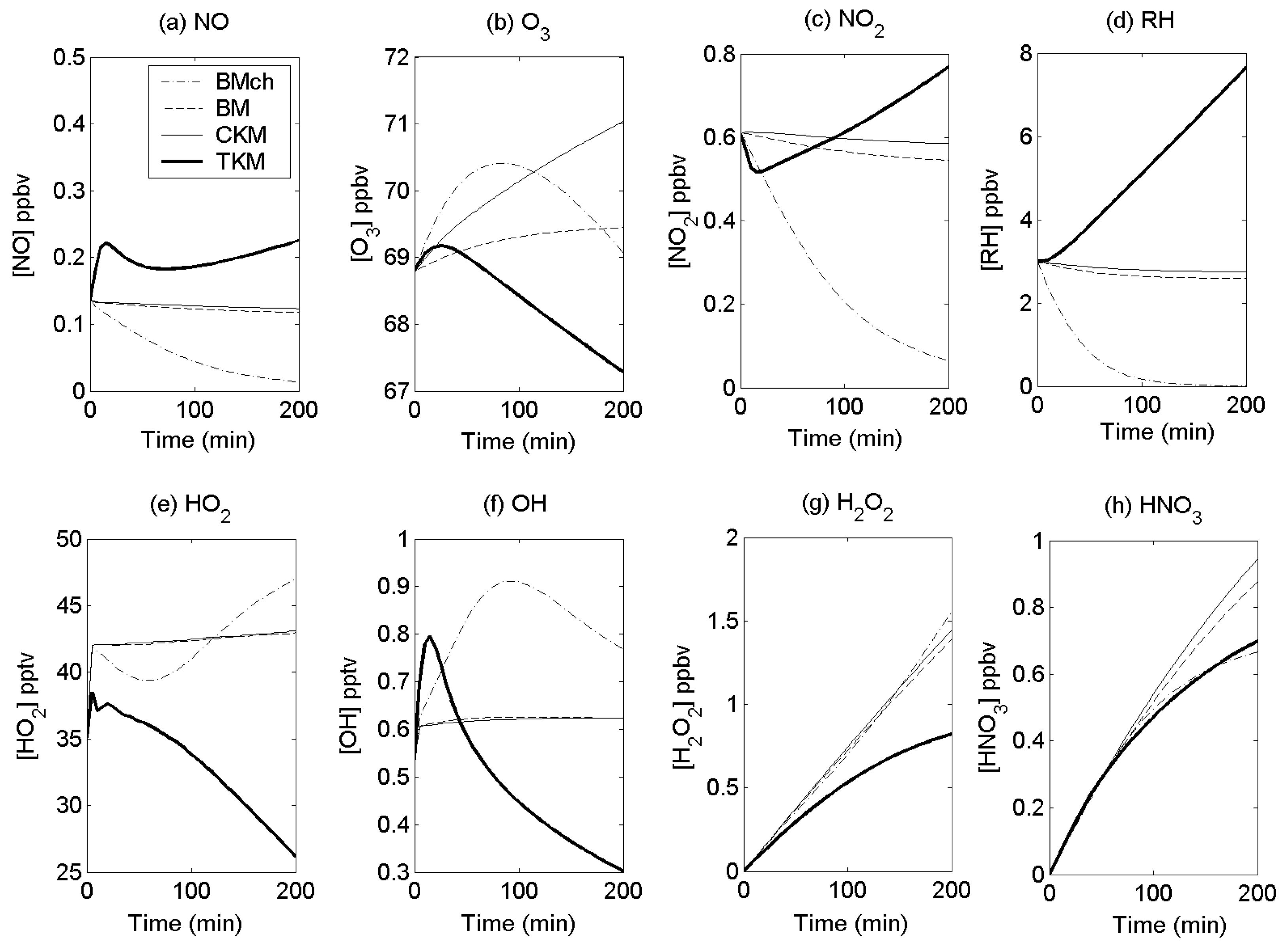
• 0-dimensional Box Model (BMch) simulating only chemical reactions with no emission or deposition fluxes.
• 0-D Box Model (BM) including chemical reactions and physical processes (emission, exchange of fluxes, and dry deposition process) but no convective transport and turbulence.
• 1-D Conventional Kinetics Model (CKM) using mean reaction rates and including transport and turbulence.
• 1-D Turbulent Kinetics Model (TKM) including transport and turbulence and using effective reaction rates.

The models operated with the same boundary and initial conditions (see Table 2) and rate constants (see Table 1). To calculate the deposition in the box model (BM), the box model concentration is used, and in the CKM and TKM, the deposition terms are calculated using the concentration in the lowest model layer.

4. Simulation Results and Discussion

4.1. Inerts

The TKM simulates the turbulent effect on chemical reaction rates by means of the concentration fields splitting method (CSM) using the extent of reaction [10]. In each simulation using the TKM, the inert species’ concentrations are first computed by setting all reaction rates equal to zero. (The reader is reminded that the term “inert” as used here refers to a model pseudo-species and not to real unreactive substances. The ’inert’ species calculation is for the same species but taking account only of their dispersion and not of the chemical reactions between them.) Then the model species’ concentrations are computed. The inert case is used to calculate indirectly the extent of reaction and also is used as a control to indicate the effects of chemical reactions on the resulting concentration profiles. The integration of the governing equations is explained in the previous study [10].

The results of the TKM for the inert species are shown in Figure 2. Their vertical profiles reveal the effects of the physical processes in the ACM. For the bottom-up diffusing concentrations of inert species NO and RH, the vertical concentration profiles were very simple and constant throughout the CBL above the surface layer as shown in Figure 2a,c. The magnitude of the emission fluxes for NO and RH cause the steep concentration gradient at the surface layer of the CBL and increase in time. Figure 2b,d reveal the concentration profiles of the inert O₃ and NO₂ simulated for the same times as in Figure 2a,c. The concentration profiles of the inert O₃ and NO₂ remain at a high concentration in the mixing layer due to the relatively slow downward transport rates in the ACM. Unlike the NO and RH, the concentrations of inert O₃ and NO₂ are reduced because there are no emission fluxes and are removed by dry deposition at the surface layer. At the upper layer of the CBL, all inert species reveal the lowest concentrations because of ventilation by the flux exchanges between the CBL and the free atmosphere (FA) which have low concentrations constantly.

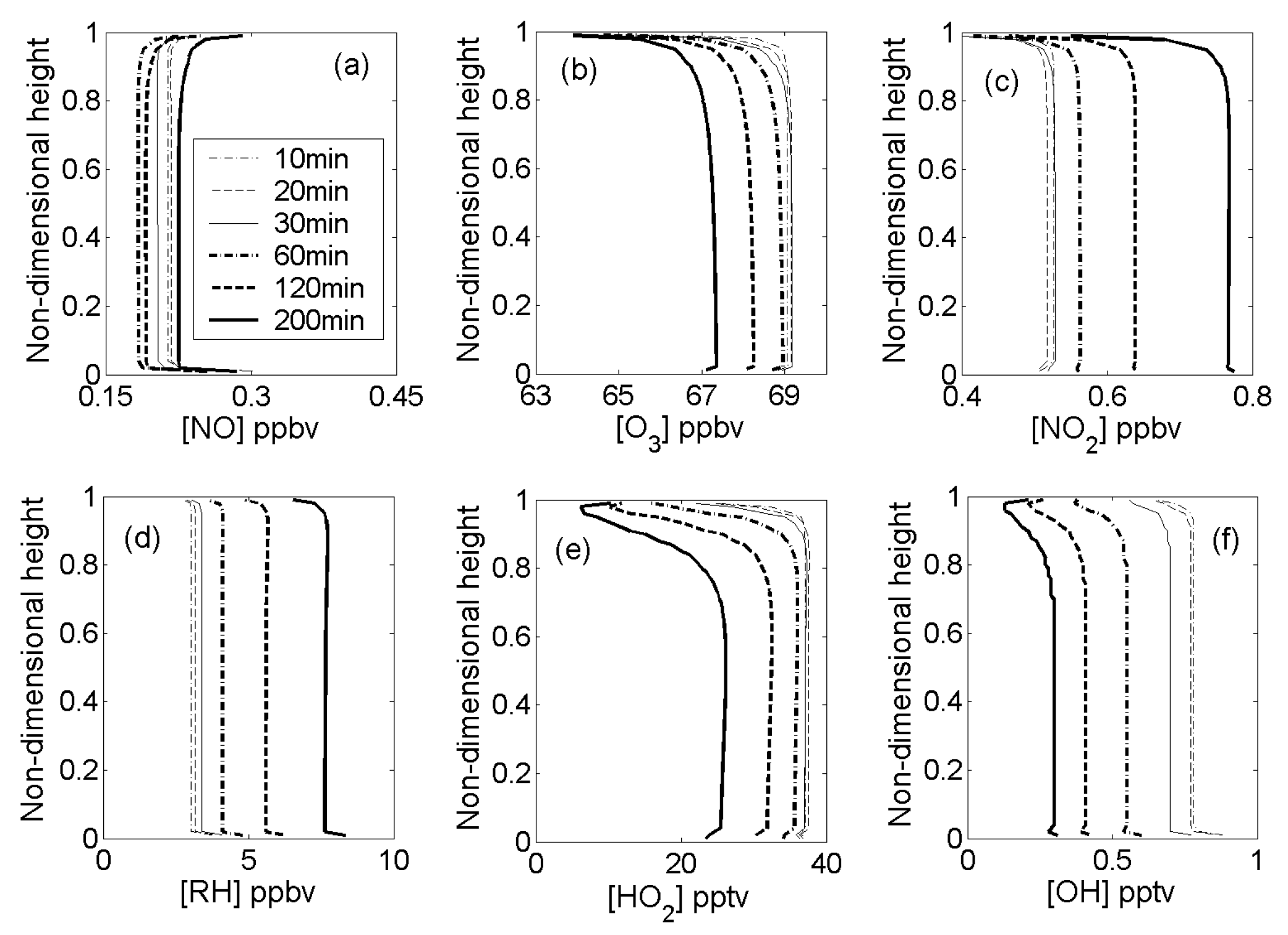
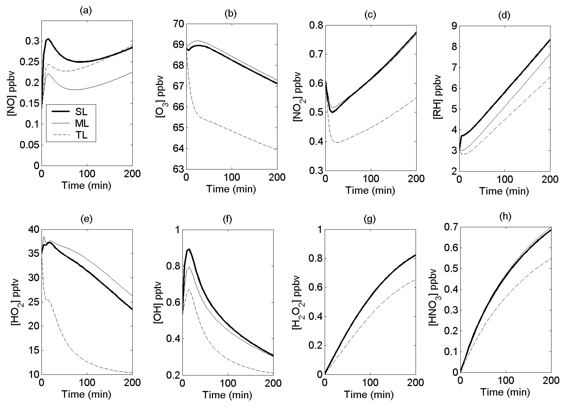
4.2. Reactive-Species Concentrations

Figure 3 shows the computed vertical concentration profiles of the reactive species in the TKM from 10 through 200 min. Rapid convective transport in the model gives rise to nearly uniform vertical concentration profiles while continued surface emissions of RH ensure that its concentrations increase steadily with time. The temporal variations of NO concentrations are more complex, as will be discussed below. The large gradients for most species near the upper and lower boundaries are due to the physical processes of emission and entrainment fluxes, surface removal, and the rapid upward convection. Figure 4 shows the temporal behavior of the six reactive species and the two end-product species H₂O₂ and HNO₃ for each of the surface, middle and top layers of the model. Here the complex early-time behavior of most of the species is clearly evident. The concentrations of the end products, H₂O₂ and HNO₃, increase monotonically out to 200 min because, in this simulation, they are created but not lost from the CBL. Their concentrations at a given time can thus be used as indications of the cumulative amounts of chemical processing.

During the first 20 min of model time, the chemical development proceeds as the emitted NO quickly starts to fill the CBL; its concentrations rise in all layers while photolysis of NO₂ serves to increase both NO and O₃ concentrations. The increase in O₃ concentrations leads to an increase in OH concentrations. This and the increasing RH concentrations lead to increasing HO₂ concentrations except in the top layer. There, the increasing NO concentrations and decreasing RH concentrations result in initially decreasing HO₂ concentrations via R₅ and R₆. At about 10 min, the HO₂ concentrations begin to increase slightly and to reach a local maximum at about 15 min. Since the HO₂ concentration is computed from the PSSAc, the behavior of HO₂ in all layers can be rationalized by examining the temporal variations of the four non-radical reactive species in Figure 4 and referring to Table 1. The same is true for the OH behavior in time. Entrainment of air from the free troposphere causes the decreasing O₃ and RH concentrations in the top layer. Note that the concentration differences in the middle layer over the interval of 0–20 min are about equal but opposite for NO and NO₂.

After 20 min, the NO concentrations decrease in all layers because of reaction with O₃; thus resulting in increases in NO₂ concentrations after the latter reach minima at 20 min. Concurrently, O₃ concentrations start to decrease at similar rates in all layers. The NO concentrations reach minima in all layers at times varying from about 40 min for the top layer to about 70 min for the surface layer. A comparison of NO and NO₂ concentration differences over appropriate intervals reveals that the stoichiometric changes for NO₂ are a little larger than for NO. For example, in the middle layer, the NO concentration decreases by about 0.05 ppb in the interval of 20–70 min, while the NO₂ concentration increases by about 0.07 ppb. During the same interval, the concentration of HNO₃ increases by more than 0.2 ppb. It is seen that a major portion (roughly about 2/3) of the NO emissions up to 70 min gets processed to HNO₃. This estimate does not take into account the effects of dry deposition of NO and NO₂.

For times greater than about 60 min NO, NO₂ and RH concentrations in all layers increase steadily while O₃, OH and HO₂ concentrations continue the decreasing trends that started after their respective early maxima. All of these changes can be understood as being driven by the emissions of NO and RH. A comparison of NO and NO₂ concentration differences over the 60–200 min. interval shows that the stoichiometric changes for NO₂ are much larger than for NO, e.g., in the middle layer where the NO concentration increases by about 0.04 ppb while the NO₂ concentration increases by about 0.22 ppb. Also during this period, the concentration of HNO₃ increases by 0.4 ppb. By 200 min, the proportion of total nitrogen species that is processed to HNO₃ is about 0.5 and the proportion of NO₂ is about 0.4 (neglecting dry deposition of NO and NO₂). Evidently, the continuing emissions of NO and RH overwhelm the ability of the oxidants to maintain their control of the growth of NO_x. Another related result shown in Figure 4 is that by 200 min the concentration of NO in the top layer slightly exceeds that in the surface layer. This is due to both the rapid transport of NO from the surface and the fact that the photolysis rate of NO₂ exceeds that of the reaction of NO with O₃ by about 8 %.

Later this study will compare the TKM results to those for other model systems to illustrate the differences caused by turbulence effects.

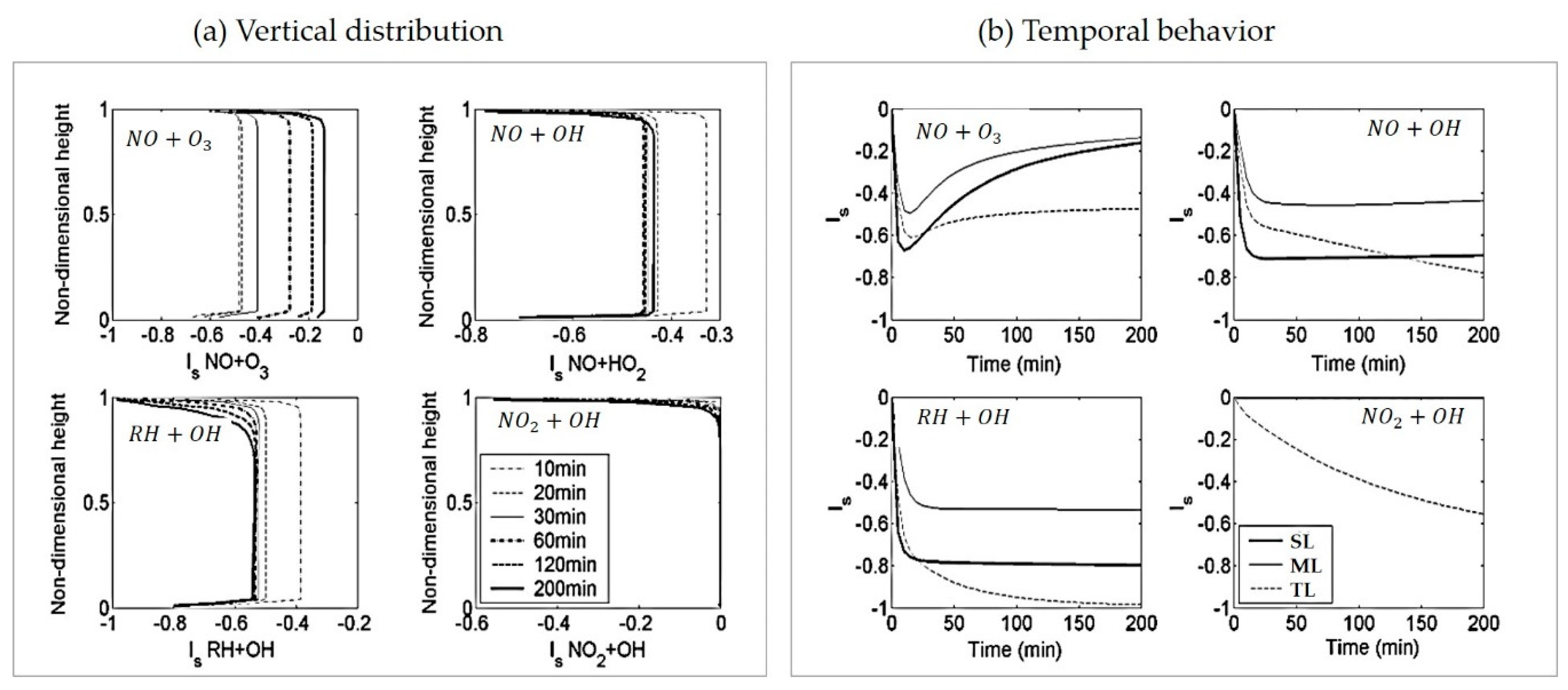
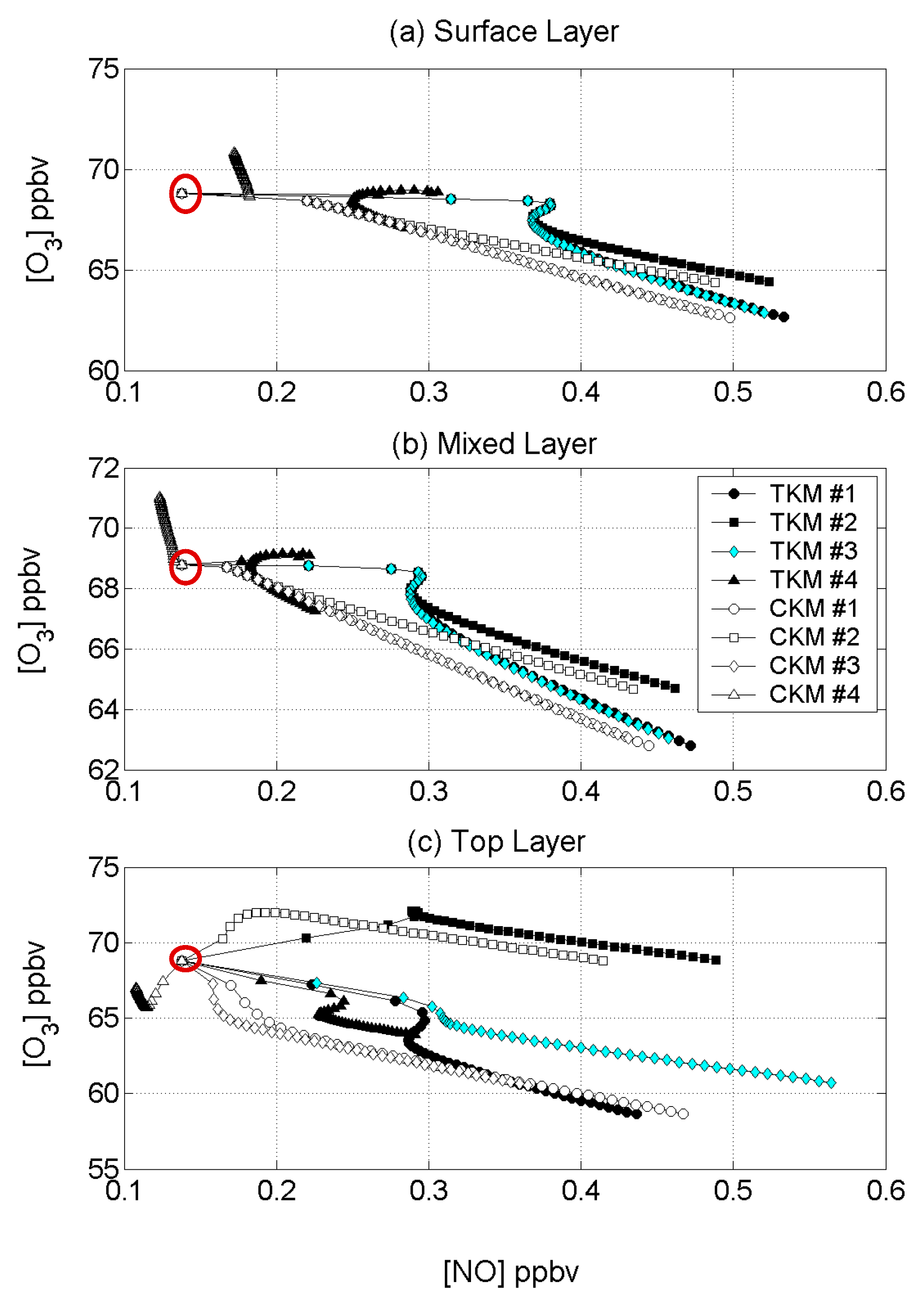
4.3. Reactant Segregation

When the chemical reaction timescale is of similar magnitude to or smaller than the turbulence timescale (${\tau }_{ch}\le {\tau }_t$), segregation of reactants becomes significant (I_s > 0 or I_s < 0); thus, the reaction rate enhances or retards. Since the coefficient of segregation, I_s, of a reaction is exactly the dimensionless (relative) covariance of the concentrations of the reactants, its value is positive when both reactants have collocated sources and is negative when the reactants originate from sources affected mainly by opposed motions.

Figure 5a shows, via the coefficient of segregation, the effects of turbulence on the reaction rates as simulated in the TKM for the reactions detailed in Table 1 (e.g., the segregation between NO and O₃, between NO and HO₂, and between RH and OH, etc.). Even though the chemical reaction chains tend to cause a balance between the production and the destruction of several species, large segregation appears for reactions involving the emitted species NO and RH. These effects permit the NO and RH concentrations to increase continuously after the early periods of decrease as discussed above. In the following discussion, the important reaction pairs have negative segregation coefficients. We will refer to their absolute values in percent, so that a minimum value in I_s is referred to as a maximum segregation. The vertical profiles (Figure 5a) of I_s for the most segregated reactions show consistency through most of the CBL. Segregations are generally larger near the top and bottom boundaries than in the bulk of the CBL. Figure 5b delineates the variation of I_s with time in the top, bottom and middle layers. For the NO + O₃ reaction, the values of I_s in all layers reach minima (largest negative values) at 20 min and then, except for the top layers, increase to about 15 %. In the top layer, segregation larger than 45 % remains at 200 min. This segregation accounts for the NO concentration in the top layer being larger than in the bottom layer. It is evident that the emission rate of NO is sufficient to keep the photochemical chain reactions from reducing the segregation of NO and O₃ to the point where average chemical kinetics prevails (I_s = 0). In the case of the RH + OH reaction, the source strength of RH is sufficient to keep segregations greater than 50% throughout the CBL after the first 20 min because HO₂ is produced by this reaction. The segregation of NO and HO₂ shows a similar pattern.

All other reaction pairs shown in Figure 6 have very small segregations (some positive and some negative) throughout the CBL with the exception of NO₂ and OH in the top layer where they increase (negatively) with time and reach about −0.55 at 200 min. The rates of those reactions with small I_s values are thus nearly what would be given by the conventional kinetic expression.

4.4. Comparisons with Other Models

Comparing the TKM to three other models further shows the effects of turbulence on the photochemical system in the CBL. The models and their characteristics are listed in Table 3. In order of complexity, these are a chemistry-only box model (BMCh), a box model (BM) and a chemical kinetics model (CKM). The results of the simulations for the middle layer of the CBL are shown in Figure 6. Since the box models have no dimensionality, the results shown in Figure 6 are merely the single sets of concentrations computed in the models. The initial concentrations of species are those of Krol et al. [25], and these were used in each simulation. The BM maintains a balance of physical and chemical processes, considering the whole CBL as a box. The physical processes simulated are emission, deposition and exchange between CBL and free atmosphere. The chemical processes are the full set of reactions given in Table 1. Since there is no turbulence and only one compartment of the CBL, the chemical kinetics terms contain only the mean concentrations. The BMCh represents only photochemistry with no emissions of NO and RH. There are no physical processes, viz. emission, deposition, exchange, transport, and turbulence. As the photochemical reactions proceed, concentrations of NO and NO₂ decrease toward zero. The CKM has all of the features of the TKM except I_s = 0. Thus, it represents the usual approach to transport and chemistry using only average concentrations of species in the reaction rate expression. Except for O₃, the results of the BM and CKM are very similar to each other for all species over the 200- min time period. For these models, the concentrations of all reacting species remain nearly constant over 200 min, except for O₃. Their slight decrease in time is caused by dry deposition.

The TKM results shown in Figure 6 are the same as those for the middle layer shown in Figure 4. The differences between the CKM and the TKM are attributable to the retarding effects of turbulence on the important reaction rates, because in the CKM, I_s = 0. Thus, the large early segregation between NO and O₃ (see Figure 5b) combined with photolysis causes the NO₂ concentrations to decrease and keep NO concentrations higher than for the CKM. The early photolysis of NO₂ contributes to the increase in O₃ and OH concentrations and thus, retards the rise of RH concentrations. However, NO–O₃ segregation, combined with the continued emissions of RH along with 50 % segregation between RH and OH, ultimately chokes off the HO_x and NO_x cycling reactions. This prevents the O₃ concentrations from increasing as they would in the CKM. Thus, the choking-off effect leaves the NO and NO₂ concentrations higher than in the CKM while the O₃ concentrations are lower. All of this is reflected also in the lower rates of buildup in the TKM of H₂O₂ and HNO₃ cumulative concentrations.

Another set of model simulations was carried out to compare the TKM with the CKM for the reversible NO_x–O₃ system [10]. In the analysis below, we also compare the results with those obtained for the NO_x–O₃–RH system. All simulation conditions in the models are the same except for the chemical mechanisms. As in the previously discussed TKM and CKM simulations, initial concentrations are 68.8 ppbv of O₃ and 0.138 ppbv of NO. Figure 7 shows the results in the form of NO–O₃ time trajectories for the bottom, middle and top layers of the CBL. Clearly the NO_x–O₃–RH chemical mechanism (triangle) shows markedly different behavior from the simple NO_x–O₃ case (diamond). The results for the NO_x–O₃–RH system are the same as previously discussed, but are presented here from a different perspective. The striking feature is that the trajectories for the CKM have distinctly different shapes and tendencies from those of the TKM in all layers. This is yet another way of portraying the segregation effects on the NO–O₃ reaction pair. They act to separate the ranges of variability of NO concentrations and to produce slightly overlapping ranges of O₃ concentrations. By contrast with those for the NO_x–O₃–RH system, the TKM and CKM trajectories for the NO_x–O₃ system, while showing early differences, are quite similar in all layers for later times. In the top layer they become parallel, separated by about 0.2 ppb NO at any time after about 20 min. The tendencies for parallel behavior are evident in the bottom and middle layers, but they approach it at later times. From the foregoing and Figure 7, it is evident that in the TKM the effect of RH sources when added to the NO sources is to constrict the range of variability of NO and O₃ concentrations.

Finally, we compare the TKM with the LES simulation [25] of the same chemical mechanism. The fundamental differences in the two approaches lie in their dimensionality (three vs. one), atmospheric dynamics, sub-grid scale parameterization, and initial times and conditions for simulation. These differences impede detailed comparisons. However, the relatively uniform vertical distributions of species and segregation coefficients and the time evolution of intensity of segregation for R₃ have significant similarities. The LES results for uniform source distribution provide generally significantly lower segregation intensities than the TKM. The TKM produced similarly low values in the sensitivity analysis when the molecular time scale was increased. Since the Damköhler number is the appropriate scaling parameter for comparing intensities of segregation, decreasing the turbulent time scale (τ_t) in the TKM would also produce similarity. However, the value of τ_t of 11 min was chosen in the TKM to be the same as in the LES. It is difficult to point to any single quantity that may account for the differences, but it seems quite probable it lies in the parameterizations that exist in both models rather than in a fundamental difference in the physical and chemical processes represented in them. There remains the difficult task of performing adequately time-resolved concentration measurements of reacting species in the turbulent convective boundary layer to determine if and to what extent turbulent segregation occurs.

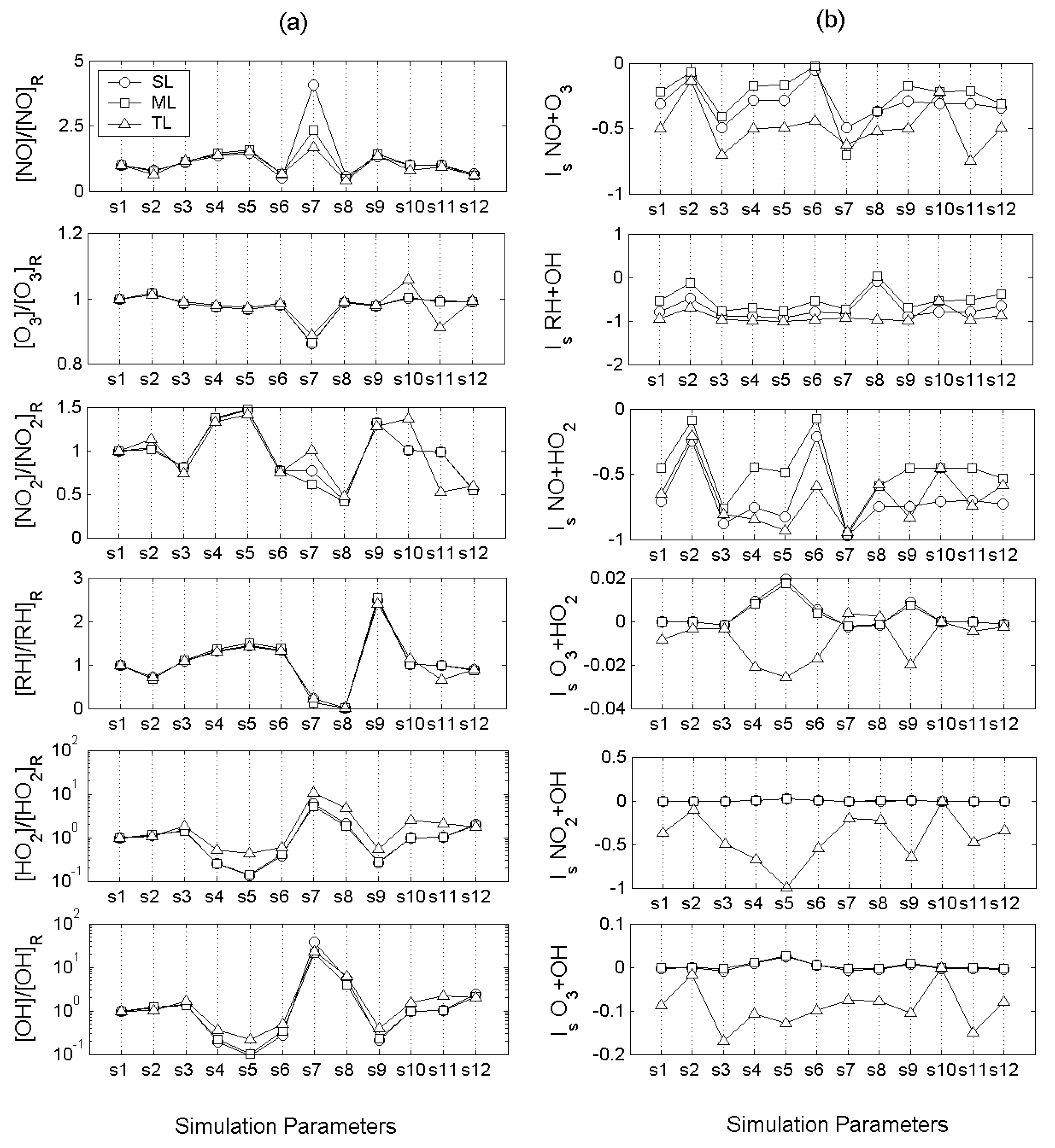
4.5. Sensitivity analysis

Table 4. Sensitivity study for various parameter values

	Molecular Timescale sec			Factor f			Reaction Rate Constants		NO Emission ppb∙m∙s−1			RH Emission ppb∙m∙s−1			Exchange Vel. at TL m∙s−1
	100	294	500	100	200	300	S90	CB-IV	0.01	0.1	1.0	0.1	1.0	10.	0.0	0.01	0.03
ref		×		×			×			×			×			×
s1	×			×			×			×			×			×
s2			×	×			×			×			×			×
s3		×			×		×			×			×			×
s4		×				×	×			×			×			×
s5		×		×			×		×				×			×
s6		×		×			×				×		×			×
s7		×		×			×			×		×				×
s8		×		×			×			×				×		×
s9		×		×			×			×			×		×
s10		×		×			×			×			×				×
s11		×		×				×		×			×			×

lists the parameters that were varied along with their values used in the sensitivity analysis of the TKM. The reference case is that which we have discussed above. Figure 8a,b show respectively the results of the sensitivity analysis in terms of the concentration ratios to the reference case of the six principal species and the coefficients of segregation (I_s) of six principal reactions at 90 min of simulated time. Note the scale changes among the plots and particularly that the OH and HO₂ concentrations scales are logarithmic.

The sensitivity analysis reveals the following:

• The concentrations of OH and HO₂ varied the most (relative to the reference case concentrations) of any other species modeled in the TKM. This is because the mechanism for the oxidation of RH and cycling of NO_x involves chain reactions with the HO_x radicals as the principal intermediates at very low concentrations between the much more abundant emitted species and their end products.
• The concentrations of NO_x, HO_x and RH modeled in the TKM were most sensitive to changes in the emission rates of NO and RH.
• Because the initial concentrations of O₃ are much larger than for the other species, they varied on an absolute basis more than any species except RH. However, because the reaction scheme is cyclical for O₃, it varied little relative to the reference case.
• The segregation effects of turbulence on R₅ and R₆ were promoted by increased emission rates of RH and NO, respectively. Decreased emission rates of those species diminished the effects of turbulence.
• The concentrations of the major species and the segregations of the principal reactions produced by the TKM appear to be relatively insensitive to the specific hydrocarbon mechanism as judged by comparing the CB-4 to the reference case [36]. Significant differences appear in HO_x species and could be expected in their end products, H₂O₂ and HNO₃, especially at later times.

5. Conclusions

The TKM successfully incorporates the “essential” chemical system using a generic hydrocarbon, RH, in conjunction with NO_x and O₃ for a typical rural agricultural regional atmosphere with RH having the same reactivity with OH as isoprene. The transport scheme in the TKM assures that significant concentration gradients exist only near the upper and lower boundaries of the CBL. Emissions of NO and RH and dry deposition of species cause gradients near the surface. The turbulence represented in the TKM produces significant segregation in the three reaction pairs among eleven reactions NO + O₃, NO + HO₂, and RH + OH for times up to 200 min. As represented in the TKM, turbulence in the CBL allows for build-up of significantly higher concentrations of NO, NO₂ and RH, while preventing the increase in O₃ concentrations compared to the CKM, in which the reactions proceed with no segregation due to turbulence. The similarity between the CKM results and those of the simple box model (BM) are nearly identical. This provides justification for the application of box model chemistry to represent the behavior of the boundary layer when turbulence effects are not included. However, the present study with the TKM indicates that turbulence effects should not be ignored in the convective boundary layer. Comparisons of the TKM with LES results are difficult because of differences in model structure and parameterizations. The LES gives lower coefficients of segregation for the principal reactions, thus representing the relatively small role of turbulence in affecting reaction rates. The TKM produces results similar to the LES for an increased molecular time scale, or equivalently, a decreased turbulent time scale. The sensitivity analysis, in which several model parameters and boundary conditions were varied, revealed less than linear changes in concentrations of the major species from changes in RH and NO emission rates. Lower emission rates lead to lower segregation effects in the principal reactions involving RH, NO and NO₂. The concentrations of the intermediate radicals OH and HO₂ are more sensitive to the variations than the more stable and abundant species. However, changing the chemical mechanism from the “essential chemistry” to CB-4 leads to relatively small changes in species concentrations and reaction segregations. Finally, it would be desirable to have a set of high-resolution time-concentration data of the key species in the CBL to provide critical comparison with the TKM and the LES model.

References

1. Weber, W.J.; DiGiano, F.A., Jr. Process Dynamics in Environmental Systems; Wiley: Hoboken, NJ, USA, 1996; Chapter 7–8; ISBN 978-0-471-01711-0. [Google Scholar]
2. Vinuesa, J.-F.; Arellano, J.V.-G.D. Fluxes and (co-)variances of reacting scalars in the convective boundary layer. Tellus B Chem. Phys. Meteorol. 2011, 55, 935–949. [Google Scholar] [CrossRef]
3. Vinuesa, J.-F.; Arellano, J.V.-G.D. Introducing effective reaction rates to account for the inefficient mixing of the convective boundary layer. Atmos. Environ. 2005, 39, 445–461. [Google Scholar] [CrossRef]
4. Fraigneau, Y.; Gonzalez, M.; Coppalle, A. The influence of turbulence upon the chemical reaction of nitric oxide released from a ground source into ambient ozone. Atmos. Environ. 1996, 30, 1467–1480. [Google Scholar] [CrossRef]
5. Sykes, R.I.; Parker, S.F.; Henn, D.S. Turbulent mixing with chemical reaction in the Planetary Boundary Layer. J. Appl. Meteorol. 1994, 33, 825–834. [Google Scholar] [CrossRef]
6. Wolfe, G.M.; Hanisco, T.F.; Arkinson, H.L.; Bui, T.P.; Crounse, J.D.; Dean-Day, J.; Goldstein, A.; Guenther, A.; Hall, S.R.; Huey, G.; et al. Quantifying sources and sinks of reactive gases in the lower atmosphere using air borne flux observations. Geophys. Res. Lett. 2015, 42, 8231–8240. [Google Scholar] [CrossRef]
7. Schumann, U. Large-eddy simulation of turbulent diffusion with chemical reactions in the convective boundary layer. Atmos. Environ. 1989, 23, 1713–1727. [Google Scholar] [CrossRef] [Green Version]
8. Donaldson, G.P.; Hilst, G.R. Effect of inhomogeneous mixing on atmospheric photochemical reactions. Environ. Sci. Technol. 1972, 6, 812–816. [Google Scholar] [CrossRef]
9. Bilger, R.W. Turbulent Flows with Nonpremixed Reactants, Turbulent Reacting Flows; Libby, P.A., Willimas, F.A., Eds.; Springer: Berlin/Heidelberg, Germany, 1980; pp. 65–113. [Google Scholar]
10. Kim, M.-S. Turbulent chemical kinetics model (TKM): A study of turbulent mixing effects on simple NOx-O3 photochemistry in Convective Boundary Layer. J. Korean Soc. Environ. Technol. 2017, 18, 86–102. [Google Scholar]
11. Seaman, N.L.; Stauffer, D.R.; Lario-Gibbs, A.M. A multiscale four-dimensional data assimilation system applied in the San Joaquin Valley during SARMAP. Part I: Modeling design and basic performance characteristics. J. Appl. Meteorol. 1995, 34, 1739–1761. [Google Scholar] [CrossRef]
12. Karamchandani, P.; Santos, L.; Sykes, I.; Zhang, Y.; Tonne, C.; Seigneur, C. Development and Evaluation of a State-of-the-Science Reactive Plume Model. Environ. Sci. Technol. 2000, 34, 870–880. [Google Scholar] [CrossRef]
13. Fu, T.-M.; Zheng, Y.; Paulot, F.; Mao, J.; Yantosca, R.M. Positive but variable sensitivity of August surface ozone to large-scale warming in the southeast United States. Nat. Clim. Chang. 2015, 5, 454–458. [Google Scholar] [CrossRef]
14. Shen, L.; Mickley, L.J.; Tai, P.K. Influence of synoptic patterns on surface ozone variability over the eastern United States from 1980 to 2012. Atmos. Chem. Phys. 2015, 15, 10925–10938. [Google Scholar] [CrossRef] [Green Version]
15. Zhang, Y.; Wang, Y. Climate-driven ground-level ozone extreme in the fall over th Southeast United States. Proc. Natl. Acad. Sci. USA 2016, 113, 10025–10030. [Google Scholar] [CrossRef] [PubMed]
16. Cleary, P.A.; Fuhrman, N.; Schulz, L.; Schafer, J.; Fillingham, J.; Bootsma, H.; McQueen, J.; Tang, Y.; Langel, T.; McKeen, S.; et al. Ozone distributions over southern Lake Michigan: Comparisons between ferry-based observations, shoreline-based DOAS observations and model forecasts. Atmos. Chem. Phys. 2015, 15, 5109–5122. [Google Scholar] [CrossRef]
17. Clifton, O.E.; Fiore, A.M.; Correa, G.; Horowitz, L.W.; Naik, V. Twenty-first century reversal of the surface ozone seasonal cycle over the northeastern United States. Geophys. Res. Lett. 2014, 41, 7343–7350. [Google Scholar] [CrossRef] [Green Version]
18. Madrigano, J.; Jack, D.; Anderson, G.B.; Bell, M.L.; Kinney, P.L. Temperature, ozone, and mortality in urban and non-urban counties in the northeastern United States. Environ. Health 2015, 14, 1–11. [Google Scholar] [CrossRef]
19. He, H.; Liang, X.-Z.; Lei, H.; Wuebbles, D.J. Future U.S. ozone projections dependence on regional emissions, climate change, long-range transport and differences in modeling design. Atmos. Environ. 2016, 128, 124–133. [Google Scholar] [CrossRef]
20. Strode, S.A.; Rodriguez, J.M.; Logan, J.A.; Cooper, O.R.; Witte, J.C.; Lamsal, L.N.; Damon, M.; Aartsen, B.V.; Steenrod, S.D.; Strahan, S.E. Trends and variability in surface ozone over the United States. JGR Atmos. 2015, 120, 9020–9042. [Google Scholar] [CrossRef] [Green Version]
21. Schnell, J.L.; Prather, M.J. Co-occurrence of extremes in surface ozone, particulate matter, and temperature over eastern North America. Proc. Natl. Acad. Sci. USA 2017, 114, 2854–2859. [Google Scholar] [CrossRef] [Green Version]
22. Khuriganova, O.; Obolkin, V.; Akimoto, H.; Ohizumi, T.; Khodzher, T.; Potemkin, V.; Golobokova, L. Long-term dynamics of ozone in surface atmosphere at remote mountain, rural and urban sites of south-east Siberia, Russia. Open Access Libr. J. 2016, 3, 1–9. [Google Scholar] [CrossRef]
23. Silva, G.D.; Graham, C.; Wang, Z.-F. Unimolecular-hydroxyperoxy radical decomposition with OH recycling in the photochemical oxidation of Isoprene. Environ. Sci. Technol. 2010, 44, 250–256. [Google Scholar] [CrossRef] [PubMed]
24. Lenschow, D.H.; Gurarie, D.; Patton, E.G. Modeling the diurnal cycle of conserved and reactive species in the convective boundary layer using SOMCRUS. Geosci. Model Dev. 2016, 9, 979–996. [Google Scholar] [CrossRef] [Green Version]
25. Krol, M.C.; Molemaker, M.J.; de Arellano, J.V.G. Effects of turbulence and heterogeneous emissions on photochemically active species in the convective boundary layer. J. Geophys. Res. 2000, 105, 6871–6884. [Google Scholar] [CrossRef] [Green Version]
26. Gao, W.; Wesely, M.L. Numerical modeling of the turbulent fluxes of chemically reactive trace gases in the atmospheric boundary layer. J. Appl. Meteorol. 1994, 33, 835–847. [Google Scholar] [CrossRef]
27. Verver, G.H.L.; van Dop, H.; Holtslag, A.A.M. Turbulent Mixing of Reactive Gases in the Convective Boundary Layer. Bound.-Layer Meteorol. 1997, 85, 197–222. [Google Scholar] [CrossRef]
28. Verver, G.H.L.; van Dop, H.; Holtslag, A.A.M. Turbulent mixing and the chemical breakdown of isoprene in the atmospheric boundary layer. J. Geophys. Res. 2000, 105, 3983–4002. [Google Scholar] [CrossRef] [Green Version]
29. Kristensen, L.; Lenschow, D.H.; Gurarie, D.; Jensen, N.O. A simple model for the vertical transport of reactive species in the convective atmospheric boundary layer. Bound.-Layer Meteorol. 2010, 134, 195–221. [Google Scholar] [CrossRef]
30. Pleim, J.E.; Chang, J.S. A non-local closure model for vertical mixing in the convective boundary layer. Atmos. Environ. 1992, 26, 965–981. [Google Scholar] [CrossRef]
31. Stockwell, R.W.; Middleton, P.; Chang, J.S.; Tang, X. The second generation regional acid deposition model chemical mechanism for regional sir quality modeling. J. Geophys. Res. 1990, 95, 16343–16367. [Google Scholar] [CrossRef]
32. Yarwood, G.; Whitten, G.Z.; Rao, S. Final Report-Updates to the Carbon Bond 4 Photochemical Mechanism, ENVRON International Corporation. Available online: http://citeseerx.ist.psu.edu/viewdoc/download?doi=10.1.1.616.4133&rep=rep1&type=pdf (accessed on 16 January 2019).
33. Lamb, R.G.; Shu, W.R. A model of second-order chemical reactions in turbulent fluid—Part I: Formulation and validation. Atmos. Environ. 1978, 2, 1685–1694. [Google Scholar] [CrossRef]
34. Georgopoulos, P.G.; Seinfeld, J.H. Mathematical modeling of turbulent reacting plumes—I. General theory and model formulation. Atmos. Environ. 1986, 20, 1791–1808. [Google Scholar] [CrossRef]
35. Ganzeveld, L.; Lelieveld, J. Dry deposition parameterization in a chemistry general circulation model and its influence on the distribution of reactive trace gases. J. Geophys. Res. 1995, 100, 20999–21012. [Google Scholar] [CrossRef]
36. Hauglustaine, D.A.; Granier, C.; Brasseur, G.P.; Megie, G. The importance of atmospheric chemistry in the calculation of radiative forcing on the climate system. J. Geophys. Res. 1994, 99, 1173–1186. [Google Scholar] [CrossRef]
37. Jacob, D.; Wofsy, S. Photochemistry of biogenic emissions over the Amazon forest. J. Geophys. Res. 1988, 93, 1477–1486. [Google Scholar] [CrossRef]
Figure 1. Schematic diagram for 1-D TKM: FA (Free Atmosphere), EZ (Entrainment Zone), ML (Middle Layer), and SL (Surface Layer): (a) Model problem (Asymmetric turbulent transport and transformation using Top-Down and Bottom-Up concept) for the free convection, (b) Vertical missing scheme (Scheme of ACM(Asymmetric Convective Model) for vertical mixing), (c) Model structure (elements of TKM), (d) Essential NOx–O3–RH Photochemistry in TKM.
Applsci 09 00357 g001
Figure 2. Vertical distribution of concentrations for inert species at 10, 20, 30, 60, 120, and 200 min. Simulation designed with emission fluxes for inert species NO and RH and no emission fluxes for inert species O3 and NO2 at the surface layer and with flux exchanges between CBL and FA for all inert species.
Applsci 09 00357 g002
Figure 3. Vertical distribution of concentrations for reactive species at 10, 20, 30, 60, 120, and 200 min. Simulation designed with emission fluxes for reactive species and no emission fluxes for other reactive species: (a) NO, (b) O3, (c) NO2, (d) RH, (e) HO2, and (f) OH at the surface layer and with flux exchanges between CBL and FA for all reactive species.
Applsci 09 00357 g003
Figure 4. Temporal behaviors of the highest concentrations of reactive species for 200 min at the surface layer (SL) [z ≤ 100 m], in the middle layer (ML) [100 < z < 900 m], and at the top layer (TL) [z ≥ 900 m] of 64 uniform vertical grids in Zi = 1000 m. The simulation is designed with emission fluxes for reactive species and no emission fluxes for the other reactive species: (a) NO, (b) O3, (c) NO2, (d) RH, (e) HO2, (f) OH, (g) HNO3, and (h) H2O2 at the surface layer, with flux exchanges between CBL and FA for all reactive species, and with no deposition velocity for the end-product species (g) HNO3 and (h) H2O2.
Applsci 09 00357 g004
Figure 5. Segregation coefficients between reactive species at three layers (surface layer, SL; middle layer, ML; top layer, TL) with times of 10, 20, 30, 60, 120, and 200 min: (a) Vertical distribution and (b) Temporal behavior
Applsci 09 00357 g005
Figure 6. Temporal behaviors of reactive species concentrations in the middle layer. Data are from the models BMch, BM, CKM, and TKM.
Applsci 09 00357 g006
Figure 7. NO-O3 trajectories at 5 min intervals to 200 min in three layers. Comparison of two models (TKM and CKM) in closed and open systems for NO–O3 and NO–O3–RH. Case #1 (simple NOx–O3 reaction; closed system; flux ratio of NO to O3 =0.1/0.1=1), Case #2 (simple NOx–O3 reaction; closed system; flux ratio of NO to O3 = 0.1/−0.1= −1), Case #3 (simple NOx-O3 reaction; open system; variable flux ratio of NO to O3), and Case #4 (essential NOx-O3-RH reaction; open system; variable flux ratio of NO to O3). Red circles mark starting points of the various trajectories.
Applsci 09 00357 g007
Figure 8. Sensitivity analysis of TKM: (a) Concentration ratio sensitivity for parameters detailed in Table 4 and (b) segregation sensitivity for the parameters detailed in Table 4.
Applsci 09 00357 g008