Tonic Cold Pain Detection Using Choi–Williams Time-Frequency Distribution Analysis of EEG Signals: A Feasibility Study

Abstract

Detecting pain based on analyzing electroencephalography (EEG) signals can enhance the ability of caregivers to characterize and manage clinical pain. However, the subjective nature of pain and the nonstationarity of EEG signals increase the difficulty of pain detection using EEG signals analysis. In this work, we present an EEG-based pain detection approach that analyzes the EEG signals using a quadratic time-frequency distribution, namely the Choi–Williams distribution (CWD). The use of the CWD enables construction of a time-frequency representation (TFR) of the EEG signals to characterize the time-varying spectral components of the EEG signals. The TFR of the EEG signals is analyzed to extract 12 time-frequency features for pain detection. These features are used to train a support vector machine classifier to distinguish between EEG signals that are associated with the no-pain and pain classes. To evaluate the performance of our proposed approach, we have recorded EEG signals for 24 healthy subjects under tonic cold pain stimulus. Moreover, we have developed two performance evaluation procedures—channel- and feature-based evaluation procedures—to study the effect of the utilized EEG channels and time-frequency features on the accuracy of pain detection. The experimental results show that our proposed approach achieved an average classification accuracy of 89.24% in distinguishing between the no-pain and pain classes. In addition, the classification performance achieved using our proposed approach outperforms the classification results reported in several existing EEG-based pain detection approaches.

1. Introduction

Pain is an unpleasant sensation that is caused by illness or physical injury. Nowadays, caregivers in the medical domain are using several methods to assess clinical pain, such as the visual analog scale (VAS), numerical rating scale (NRS), and verbal rating scale (VRS) [1]. These clinical pain assessment methods require the caregiver to perform an interview with the patient to determine the level of pain. Therefore, such pain assessment methods are considered subjective as the pain tolerance level can vary significantly among different patients. Moreover, these methods are not suitable for patients who are unable to verbally express pain, such as infants [2]. This justifies the importance of developing objective pain assessment methods that can detect pain by analyzing the brain signals of the patients. In fact, objective pain detection methods can provide caregivers with a second opinion that can enhance the assessment and management of clinical pain.

In order to study the pain perception mechanism, researchers have recently worked on analyzing brain activities that are recorded for healthy subjects under stimulated pain conditions. Among the different types of pain stimuli, tonic pain stimuli are widely used due to their high induced effects compared to the other types of pain stimuli. In particular, tonic pain can cause impairments in the performance of visual tasks and memory [3,4]. Moreover, various studies have indicated that tonic pain can simulate clinical pain better than other types of pain stimuli [8].

To record brain activities that are generated in response to an exogenous pain stimulus, researchers have employed several neuroimaging modalities, such as the electrocorticographic (ECoG), functional magnetic resonance imaging (fMRI), functional near-infrared spectroscopy (fNIRS), and electroencephalography (EEG). The EEG modality, which records the electrical potentials produced at different locations in the brain in response to an exogenous pain stimulus, is considered the most commonly used modality for designing objective pain detection systems. This can be attributed to several properties that are associated with the EEG modality, including the high temporal resolution, low-cost, and noninvasive nature [5,6]. Nonetheless, pain detection based on EEG signals analysis is considered challenging due to the nonstationarity nature of the EEG signals, low spatial resolution, and low signal-to-noise (SNR) ratio [7].

Over the past decade, several approaches have been proposed to detect stimulated pain based on EEG signals analysis. For example, Nir et al. [8] studied the relation between the properties of the peak alpha frequency (PAF) of the EEG signals and the subjective perception of tonic heat pain. The employed EEG signals were recorded for 18 healthy subjects during the application of tonic heat pain stimulus. The results indicate a correlation between the PAF and the subjective perception of tonic pain, which suggests the possibility of utilizing the properties of the PAF to characterize pain. Panavaranan and Wongsawat [9] proposed an approach to detect tonic heat pain using power spectral density (PSD)-based features that were extracted from the EEG signals. The extracted features were used to construct a support vector machine (SVM) classifier to distinguish between EEG signals that correspond to the no-pain and pain classes, respectively. The performance of the proposed system was evaluated using EEG signals that were acquired from nine healthy subjects during the application of tonic heat pain stimulus. Shao et al. [10] performed a frequency-domain EEG source analysis to study brain responses to tonic cold pain stimulus. In particular, the utilized EEG signals were recorded for 26 healthy subjects under two conditions—absence or presence of a tonic cold pain stimulus. The results show that the variations in the power associated with different frequency bands of the EEG signals can be used to analyze the perception mechanism of tonic cold pain. In another study, Vatankhah and Toliyat [11] proposed an approach that employs the wavelet coherency to estimate the tonic cold pain level. In particular, first- and second-order statistical features were extracted from the wavelet coherency of the EEG signals and used to construct two classifiers— an SVM classifier with radial basis function (RBF) kernel and a hidden Markov model (HMM) classifier. The results indicate that the classification performance obtained using the SVM classifier outperform the classification results obtained using the HMM classifier.

The previously described studies were focused on analyzing the EEG signals in the frequency- domain without considering the nonstationarity nature of these signals. The nonstationarity nature of the EEG signals imposes the requirement of analyzing these signals in the joint time-frequency domain to capture the spectral variations of the EEG signals over time. In this regard, few research groups have recently investigated the use of time-frequency analysis methods, such as wavelet transform [12,13], to characterize the EEG signals and detect tonic pain. For example, Hadjileontiadis [14] utilized the continuous Wavelet transform (CWT) to analyze the EEG signals and detect tonic cold pain. In particular, the CWT was employed to construct a time-frequency representation of the EEG signals. Then, a set of higher-order spectral features were extracted and used to train and evaluate the performance of four different classifiers, namely the quadratic discriminant analysis (QDA), Mahalanobis (MAH), k-nearest neighbor (k-NN), and SVM with RBF kernel classifiers. The performance of these classifiers was evaluated using EEG signals acquired from 17 healthy subjects while holding a plastic bottle with iced water until the pain became unbearable. The experimental results indicate that the best classification accuracy was achieved using the MAH classifier. In another study, Alazrai et al. [15] proposed a tonic cold pain detection approach that utilizes the discrete Wavelet transform (DWT) to analyze the EEG signals and detect pain. This approach was evaluated using EEG signals that were acquired from 24 healthy subjects while submerging their hands in iced water to stimulate tonic cold pain. The DWT was applied to the recorded EEG signals, and a set of features were extracted from the computed DWT coefficients. The extracted features were used to train a SVM classifier with RBF kernel to distinguish between the EEG signals that correspond to the no-pain and pain states. Despite the promising results achieved using the Wavelet transform analysis of the EEG signals, including CWT and DWT, the time-frequency representations obtained using the Wavelet transform are characterized by a nonuniform resolution across the time-frequency plane (TFP) [16], which can increase the difficulty to interpret the obtained time-frequency representation of the EEG signals [16,17].

To address the limitations of the previously described EEG-based pain detection approaches, we propose an EEG-based pain detection approach that employs a quadratic time-frequency distribution, namely the Choi–Williams distribution (CWD), to analyze the EEG signals. Compared to other time-frequency analyses, such as the Wavelet transform, the QTFDs are considered invariant to time and frequency shifts [16,18,19]. Therefore, the use of the CWD enables construction of a time-frequency representation (TFR) of the EEG signals that can capture the time-varying spectral characteristics of the EEG signals. To reduce the dimensionality of the TFRs constructed for the EEG signals, we have extracted 12 time-frequency features from the constructed TFR of the EEG signals. These extracted time-frequency features are used to train a support vector machine (SVM) classifier to distinguish between EEG signals that are associated with pain and no-pain states. To evaluate the performance of the proposed approach, we have recorded the EEG signals for 24 healthy subjects who volunteered to participate in a tonic cold pain stimulation experiment. Moreover, we have developed two performance evaluation procedures—channel- and feature-based analyses—to evaluate the effect of the selected EEG channels and time-frequency features on the capability of detecting pain. The results reported in the current study demonstrate the capability of our proposed approach to detect tonic cold pain using EEG signals.

The main objective of the current study is to contribute to ongoing research efforts developing objective pain detection systems based on time-frequency analysis of the EEG-based pain detection. In particular, we have introduced an EEG-based system that employs a set of time-frequency features that are extracted from a QTFD-based representation to discriminate between the no-pain and pain classes. In fact, we hypothesize that analyzing the EEG signals using the CWD, which is considered as a QTFD, can improve the accuracy of pain detection compared with other previously used frequency-domain and time-frequency domain analyses, such as the PSD-based analysis and the wavelet transform (WT) analysis. The contribution of this study is three-fold: (1) To the best of our knowledge, this is the first study that employs the CWD to analyze EEG signals for detecting pain. Therefore, our work can be viewed as a feasibility study that aims to explore the potential of developing objective clinical pain detection systems based on time-frequency analysis of the EEG signals. (2) A novel set of time-frequency features are extracted from the constructed CWD-based TFR of the EEG signals to model the no-pain and pain classes encapsulated within the EEG signals, (3) Extensive feature and channel selection analyses are performed to quantify the effect of excluding any of the extracted time-frequency features and any of the utilized EEG channels on the accuracy of pain detection.

The remainder of the paper is structured as follows. In Section 2, we describe the experimental protocol, the recorded EEG signals, the CWD-based time-frequency analysis, the extraction and classification of the features, and the performance evaluation procedures. In Section 3, we present and discuss the results. In Section 4, we conclude our findings and provide future directions.

2. Materials and Methods

2.1. Subjects

Twenty four healthy subjects (12 females and 12 males, with a mean ± standard deviation age of 22.5 ± 3.2 years) volunteered to participate in this study. The subjects were not feeling any pain before participating in the experiment and not taking any medication related to neurological or psychiatric disorders. Moreover, each subject received a detailed explanation of the experimental protocol, which was approved by the Research Ethics Committee at the German Jordanian University, and signed a consent form before participating in the experiment.

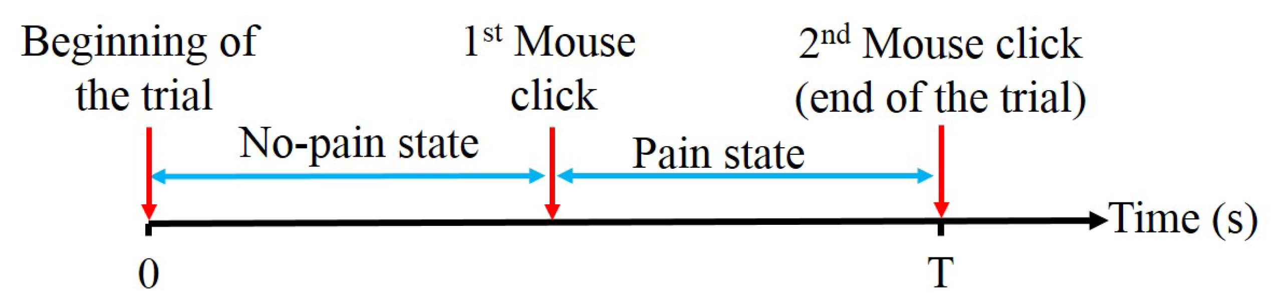
2.2. Experimental Protocol

In this study, each subject was asked to sit on a comfortable chair at a distance of approximately 50 cm from a screen displaying a black image. The subjects were instructed to keep their eyes open during the experiments. At the beginning of each EEG recording trial, the subject was asked to relax his/her right hand on a table for 15 s. Then, the subject was instructed to submerge his/her right hand in a bucket of iced water with a temperature of approximately $1.5\pm 2.5{}^{\circ }$C until he/she starts to have a moderately uncomfortable feeling. The subject marks this moment by clicking the mouse button of the recording computer using his/her left hand. This mouse click indicates the end of the no-pain state and the beginning of the pain state. During the pain state, the subject keeps his/her hand submerged in the bucket of the iced water until the pain becomes intolerable. At this moment, the subject withdraws his/her right hand from the iced water and relaxes it on the table. The pain state ends when the subject feels that the pain has reduced to a moderate level by clicking the mouse button again to indicate the end of the trial and EEG recording. After each trial, the subject was asked to submerge his/her right hand in a bucket of warm water that had a temperature of $40\pm 1{}^{\circ }$C and countdown for 3 s starting from a random 4-digit number to ensure that each trial begins with the no-pain state [20]. The total number of trails recorded for each subject is five trials. Moreover, the average ± standard deviation duration of each trial computed over all subjects is $65.8\pm 19.1$ s. Figure 1 shows the timing diagram of the experimental procedure during each trial.

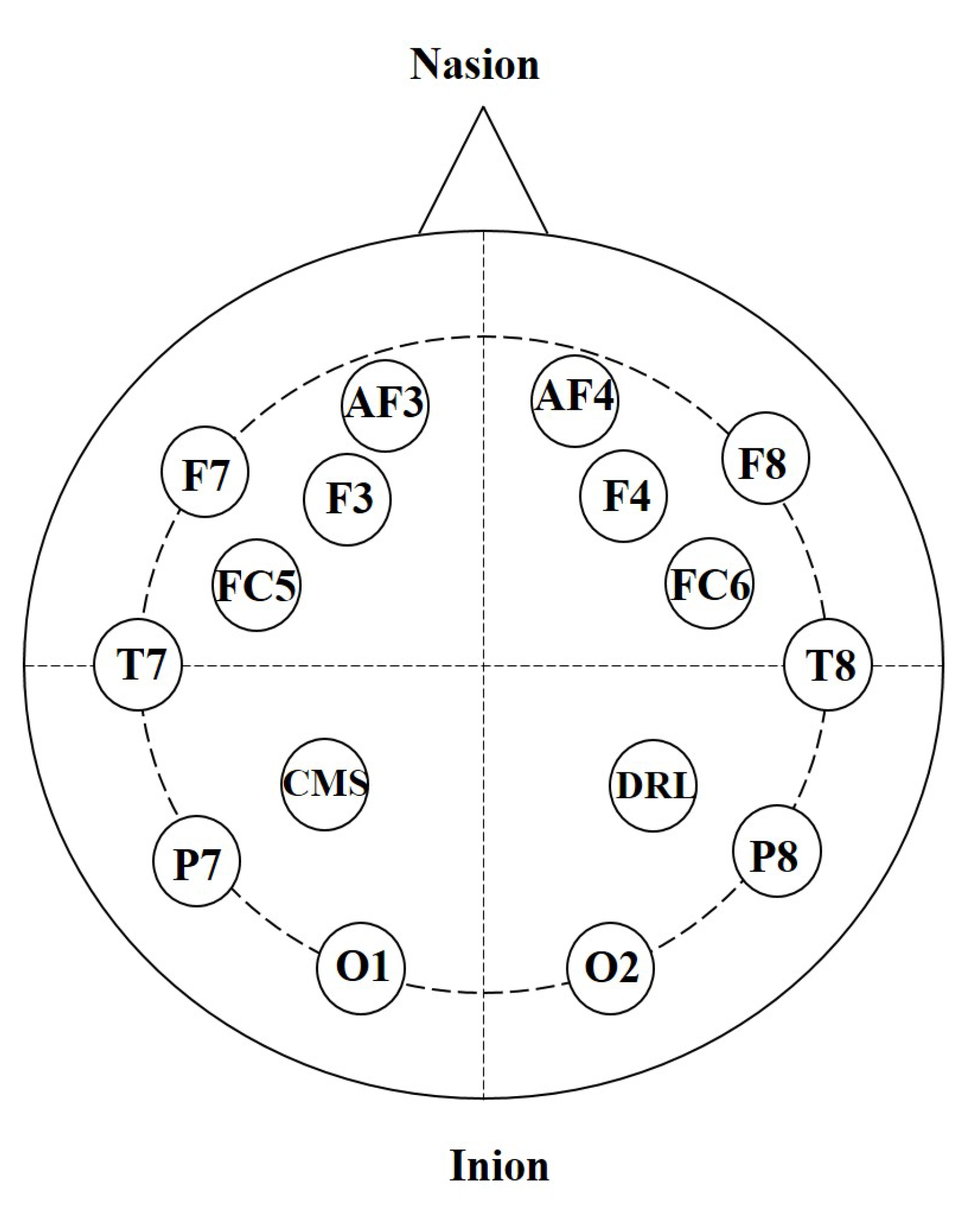
2.3. Data Acquisition and Preprocessing

The EEG signals were recorded using the Emotiv EPOC+ EEG neuroheadset system (https://www.emotiv.com). The Emotiv system consists of 14 EEG electrodes that are arranged on the scalp according to the 10–20 international electrode placement system at the following locations; $F_7$, $T_7$, $A{F}_3$, $O_1$, $F_4$, $P_7$, $A{F}_4$, $F_8$, $F_3$, $P_8$, $O_2$, $F{C}_5$, $T_8$, and $F{C}_6$. These electrodes are referenced to the common mode sense (CMS)/ driven right leg (DRL) at the $P_3$ and $P_4$ locations. Figure 2 shows the positions of the EEG electrodes on the scalp. The acquired EEG signals are internally sampled at a frequency of 2048 Hz. Moreover, the Emotiv system is configured to filter the recorded EEG signals using a hardware band-pass filter with a bandwidth of 0.2 to 43 Hz and downsamples the EEG signals to 128 samples per second. Finally, the muscle and electrooculography artifacts within the EEG signals are reduced using the automatic artifact removal (AAR) toolbox [21,22].

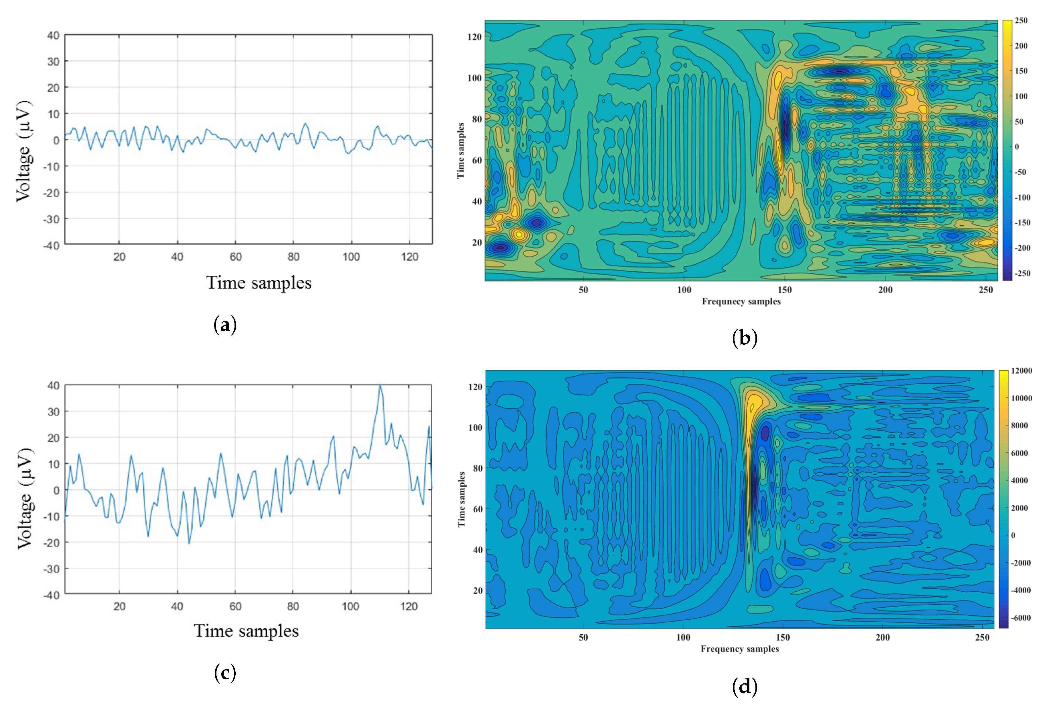
2.4. Time-Frequency Analysis of the EEG Signals

The EEG signals are nonstationary signals due to their time-varying spectral components [6,17,23]. This implies that analyzing the EEG signals in the time-domain or the frequency-domain may not capture the variations in the spectral characteristics of the EEG signals over time [24]. In this regard, researchers have utilized several time-frequency analysis techniques to construct TFRs of the nonstationary signals, such as the wavelet transform (WT) [13]. Despite the promising results obtained based on analyzing the EEG signals using the WT [14,25], the TFRs constructed using the WT method have a nonuniform resolution across the time-frequency plane and are considered variant to frequency-shifts [16]. Having that said, in this study, we propose the use of a QTFD, namely the Choi–Willimas Distribution (CWD) [26], to analyze the EEG signals. The CWD maps the time-domain EEG signals into a high-resolution time-frequency domain that quantifies the distribution of the energy encapsulated in the EEG signals over the time and frequency domains [16,17,26].

To compute the CWD, we utilized a sliding window approach to divide the EEG signal of each electrode into a set of overlapping segments. Specifically, the number of samples within each segment is equal to 128 samples and the overlap between consecutive segments is equal to 64 samples. Then, for each EEG segment, $x\left(t\right)$, the CWD of $x\left(t\right)$, denoted by ${\mathsf{\Gamma }}_x(t,f)$, can be computed as follows [16,17].

$${\mathsf{\Gamma }}_x(t,f)=W_x{(t,f)}_{\genfrac{}{}{0pt}{}{\ast \ast }{(t,f)}}\mathsf{\Phi }(t,f),$$

(1)

where t and f represent the indices of the time and frequency samples, respectively, $W_x(t,f)$ is the Winger–Ville distribution (WVD) of $x\left(t\right)$, $\genfrac{}{}{0pt}{}{\ast \ast }{(t,f)}$ is the two-dimensional (2D) convolution operation computed over time and frequency domains, and $\mathsf{\Phi }(t,f)$ represents a time-frequency smoothing kernel. Specifically, the WVD of $x\left(t\right)$, $W_x(t,f)$, can be computed as follows [17].

$$W_x(t,f)={\int }_{-\infty }^{\infty }a(t+\frac{\nu }{2})a^{\ast }(t-\frac{\nu }{2})e^{-j2\pi f\nu }\partial \nu ,$$

(2)

where $a\left(t\right)=x\left(t\right)+j\mathcal{H}\left\{x\right(t\left)\right\}$ is the analytic signal associated with $x\left(t\right)$, $\mathcal{H}$ is the Hilbert transform [27], and $a^{\ast }(·)$ is the complex conjugate of $a(·)$. Moreover, the time-frequency smoothing kernel, $\mathsf{\Phi }(t,f)$, can be expressed as follows [26].

$$\mathsf{\Phi }(t,f)=exp\left(-\frac{t^2{f}^2}{{\alpha }^2}\right),$$

(3)

where $\alpha >0$ is a smoothing parameter that determines the amount of suppression applied to the cross-terms introduced by the WVD and its value was experimentally tuned to be 0.7. In this work, we have utilized the HOSA toolbox [28] to compute the CWD of the EEG segments. The dimensionality of the CWD-based time-frequency representation (TFR) computed for each EEG segment, which is obtained using Equation (1), is equal to $T\times F$, where $T=128$ represents the number of time samples within an EEG segment and $F=256$ represents the number of frequency samples. Figure 3 provides sample images of the CWD-based TFR constructed for two different EEG segments. In particular, Figure 3a shows an EEG segment that belongs to the no-pain class. The CWD-based TFR constructed for the EEG segment presented in Figure 3a is shown in Figure 3b. Similarly, Figure 3c shows an EEG segment that belongs to the pain class. Figure 3d shows the CWD-based TFR constructed for the EEG segment presented in Figure 3c.

2.5. Feature Extraction

To reduce the dimensionality of the constructed CWD-based TFR, we propose to extract a set of twelve time-frequency features, denoted as TF${}_1$–TF${}_{12}$, which quantify the CWD-based TFR computed for each EEG segment.

Table 1. The time-frequency features extracted from the CWD-based TFR of each EEG segment [6,7,23].

Time-Frequency Feature	Mathematical Expression of the Time-Frequency Feature
The mean of the CWD ($T{F}_1$)	$$T{F}_1=\frac{1}{T\times F}\sum _{t=1}^T\sum _{f=1}^F{\mathsf{\Gamma }}_x(t,f)$$ (4)
The variance of the CWD ($T{F}_2$)	$$T{F}_2=\frac{1}{T\times F}\sum _{t=1}^T\sum _{f=1}^F{({\mathsf{\Gamma }}_x(t,f)-T{F}_1)}^2$$ (5)
The skewness of the CWD ($T{F}_3$)	$$T{F}_3=\frac{1}{T\times F\times {\left(T{F}_2\right)}^{3/2}}\sum _{t=1}^T\sum _{f=1}^F{({\mathsf{\Gamma }}_x(t,f)-T{F}_1)}^3$$ (6)
The kurtosis of the CWD ($T{F}_4$)	$$T{F}_4=\frac{1}{T\times F\times {\left(T{F}_2\right)}^2}\sum _{t=1}^T\sum _{f=1}^F{({\mathsf{\Gamma }}_x(t,f)-T{F}_1)}^4$$ (7)
Sum of the logarithmic amplitudes of the CWD ($T{F}_5$)	$$T{F}_5=\sum _{t=1}^T\sum _{f=1}^{F}log\left(\right|{\mathsf{\Gamma }}_x(t,f)\left|\right)$$ (8)
Median absolute deviation of the CWD ($T{F}_6$)	$$T{F}_6=\frac{1}{T\times F}\sum _{t=1}^T\sum _{f=1}^F|{\mathsf{\Gamma }}_x(t,f)-T{F}_1|$$ (9)
Root mean square value of the CWD ($T{F}_7$)	$$T{F}_7=\sqrt{\left(\sum _{t=1}^T\sum _{f=1}^F{\mathsf{\Gamma }}_x(t,f)\right)/(T\times F)}$$ (10)
interquartile range of the CWD ($T{F}_8$)	$$T{F}_8=\frac{1}{F}\sum _{f=1}^F\left({\mathsf{\Gamma }}_x\left(\frac{3(T+1)}{4},f\right)-{\mathsf{\Gamma }}_x\left(\frac{(T+1)}{4},f\right)\right)$$ (11)
The flatness of the CWD ($T{F}_9$)	$$T{F}_9=T\times F\times \frac{{\prod }_{t=1}^T{\prod }_{f=1}^F\left(\right|{\mathsf{\Gamma }}_x(t,f){\left|\right)}^{1/T\times N}}{{\sum }_{t=1}^T{\sum }_{f=1}^F\left(\right|{\mathsf{\Gamma }}_x(t,f)\left|\right)}$$ (12)
The flux of the CWD ($T{F}_{10}$)	$$T{F}_{10}=\sum _{t=1}^{T-1}\sum _{f=1}^{F-1}({\mathsf{\Gamma }}_x(t+1,f+1)-{\mathsf{\Gamma }}_x(t,f))$$ (13)
The normalized Renyi entropy of the CWD ($T{F}_{11}$)	$$T{F}_{11}=\frac{1}{1-3}{log}_2\sum _{t=1}^T\sum _{f=1}^F{\left(\frac{{\mathsf{\Gamma }}_x(t,f)}{T\times F\times T{F}_1}\right)}^3$$ (14)
The energy concentration of the CWD ($T{F}_{12}$)	$$T{F}_{12}={\left(\sum _{t=1}^T\sum _{f=1}^F\sqrt{|{\mathsf{\Gamma }}_x(t,f)|}\right)}^2$$ (15)

describes the twelve time-frequency features extracted from the CWD-based TFR of each EEG segment. The first eight features, TF${}_1$–TF${}_8$, are computed by extending eight time-domain features to the joint time-frequency domain. These eight features are the mean ($T{F}_1$), variance ($T{F}_2$), skewness ($T{F}_3$), kurtosis ($T{F}_4$), sum of the logarithmic amplitudes ($T{F}_5$), median absolute deviation ($T{F}_6$), root mean square value ($T{F}_7$), and interquartile range ($T{F}_8$) values computed for the constructed CWD-based TFR of each EEG segment. The aforementioned eight time-frequency features comprise higher-order statistical features, such as $T{F}_3$ and $T{F}_4$, which characterize the distribution of the energy encapsulated in an EEG segment. The last four features, $T{F}_9$–$T{F}_{12}$, are obtained by extending four frequency-domain features to the joint time-frequency domain. These four features are the flatness ($T{F}_9$), flux ($T{F}_{10}$), normalized Renyi entropy ($T{F}_{11}$), and energy concentration ($T{F}_{12}$) values computed for the constructed CWD-based TFR of each EEG segment. The last four features in Table 1 quantify the time-variant spectral information within each EEG segment. Detailed description of the construction procedure and the physical interpretation of the extracted time-frequency features can be found in our previous work [6,7,23].

The time-frequency features extracted from the CWD-based TFRs of the EEG segments associated with a given temporal position of the sliding window are grouped to form a feature vector. In particular, the number of features comprised within each feature vector is equal to $14\times 12$, where 14 represents the number of EEG segments at each window position, which is equal to the number of EEG electrodes, and 12 represents the number of time-frequency features extracted from the CWD-based TFR computed for each EEG segment at a particular window position.

2.6. Classification

For each trial, the feature vectors extracted from the EEG segments associated with the window positions that are located before the first mouse click are labeled as no-pain class, while the feature vectors extracted from the EEG segments associated with the window positions that are located after the first mouse click are labeled as pain class. These labeled feature vectors are used to construct a binary support vector machine (SVM) classifier with a radial basis function (RBF) kernel [29] to classify the feature vectors into one of two pain-related classes: no-pain and pain. Specifically, for each subject, we utilize a ten-fold cross-validation procedure to train and test the constructed binary SVM classifier. The ten-fold cross-validation procedure is repeated for ten times and the average classification performance for each subject is computed over the ten repetitions. Moreover, a grid search is performed to tune the regularization parameter, C, and the RBF kernel parameter, $\gamma$, of the SVM classifier. In particular, we select the values of C and $\gamma$ that maximize the classification accuracy [30].

2.7. Performance Evaluation

In order to evaluate the effect of the utilized EEG channels and CWD-based time-frequency features on the classification performance of our proposed pain detection approach, we have developed two performance evaluation procedures: the channel- and feature-based evaluation procedures. The channel-based evaluation procedure investigates the effect of selecting a subset of the EEG channels on the accuracy of detecting pain, while the feature-based evaluation procedure investigates the effect of selecting a subset of the extracted CWD-based time-frequency features on the accuracy of detecting pain. In particular, for the channel-based evaluation procedure, we start by computing the classification performance of our proposed approach using all the EEG channels and all the CWD-based time-frequency features. After that, we apply an iterative channel reduction procedure to specify the minimum number of EEG channels required to accurately detect pain. The number of iterations of the channel reduction procedure is equal to the number of EEG channels considered in this study, which is equal to 14 channels. For each iteration, the average classification performance is computed over all subjects after removing one of the EEG channels. Then, the EEG channel that produced the highest average classification performance after its elimination is removed from subsequent iterations. Similarly, for the feature-based evaluation procedure, we applied an iterative feature reduction procedure to specify the minimum number of time-frequency features required to accurately detect pain. The number of iterations of the feature reduction procedure is equal to the number of time-frequency features considered in this study, which is equal to 12. For each iteration, the average classification performance is computed over all subjects after removing one of the CWD-based time-frequency features. Then, the time-frequency feature that produced the highest average classification performance after its elimination is removed from subsequent iterations. It is worth noting that the iterative reduction procedure, which is employed in the current channel- and feature-based performance evaluation analyses, has been successfully employed in several previous studies [31,32] as an alternative approach to the computationally-intensive exhaustive search procedure [33,34].

In addition, we compare the classification performance obtained using the CWD-based time-frequency features presented in the current study with the classification performances obtained using the features presented in the works of the authors of [8,9]. In particular, Nir et al. [8] utilized the peak alpha frequency, which represents the frequency value associated with the highest power spectral density (PSD) within the alpha frequency band, as a feature to characterize the tonic pain in the EEG signals. To compare the classification performance obtained using our proposed CWD-based time-frequency features with the classification performance obtained using the feature presented in the study by Nir et al. [8], we applied the sliding window approach described in Section 2.4 to the EEG signals employed in the current study. After that, we computed the peak alpha frequency feature for each EEG segment. The features extracted from the EEG segments associated with a particular window position are grouped to form a feature vector. Then, for each subject, we train a SVM classifier to classify the feature vectors into one of two pain-related classes—the no-pain class and pain class—using the cross-validation procedure described in Section 2.6. Similarly, Panavaranan and Wongsawat [9] utilized two features—the normalized PSD of the alpha and beta frequency bands—to characterize the tonic pain in the EEG signals. To compare the classification performance obtained using our proposed CWD-based time-frequency features with the classification performance obtained using the features presented in the study by Panavaranan and Wongsawat [9], we applied the sliding window approach described in Section 2.4 to the EEG signals employed in the current study. After that, we computed the normalized PSD of the alpha and beta frequency bands for each EEG segment. The features extracted from the EEG segments associated with a particular window position are grouped to form a feature vector. Then, for each subject, we train a SVM classifier to classify the feature vectors into one of two pain-related classes, namely the no-pain class and pain class, using the cross-validation procedure described in Section 2.6.

In this study, we compute the classification performance for each subject in terms of two standard evaluation metrics, namely the classification accuracy and the $F_1-$measure. These metrics are computed as follows [7,35].

$$Accuracy=\frac{(tp+tn)}{(tp+tn+fp+fn)}\times 100\%,$$

(16)

$$F_1-measure=2\times \frac{(PRE\ast REC)}{(PRE+REC)}\times 100\%,$$

(17)

where $tp$, $tn$, $fp$, and $fn$ are the number of true positive, true negative, false positive, and false negative cases, respectively. Moreover, $PRE=tp/(tp+fp)$ and $REC=tp/(tp+fn)$ represent the precision and recall, respectively.

3. Experimental Results and Discussion

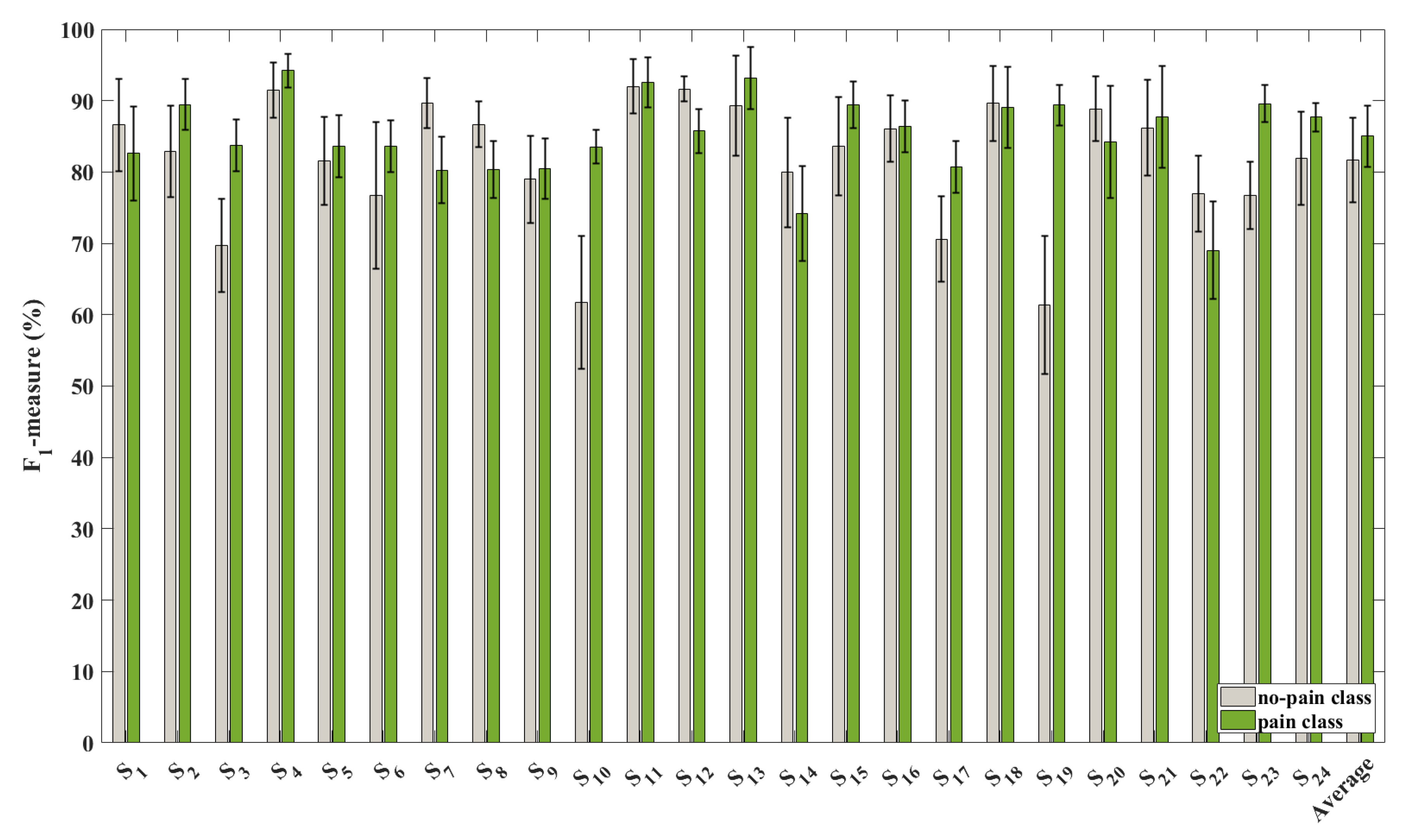
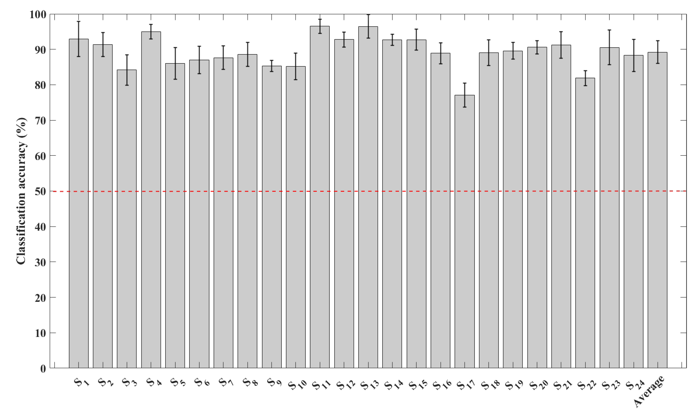
3.1. Results of the Channel-Based Evaluation Procedure

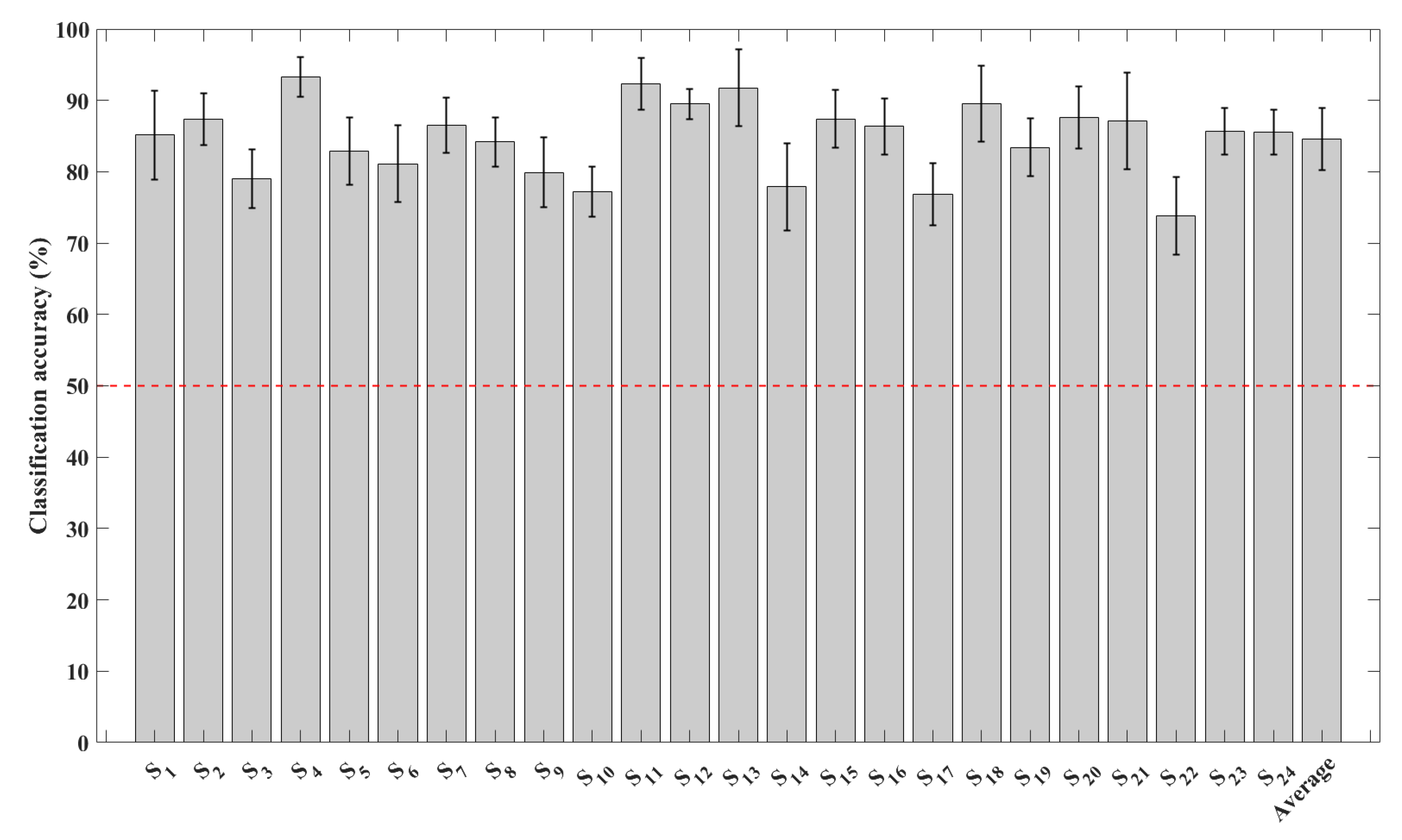
3.1.1. Results Obtained Using All the EEG Channels

In this section, we present the results obtained for our proposed approach using all the EEG channels and all the CWD-based time-frequency features. The average ± standard deviations classification accuracies obtained for each one of the 24 subjects ($S_1$–$S_{24}$) are shown in Figure 4. In particular, the average classification accuracy values computed for the 24 subjects is between 73.8%, which was obtained for $S_{22}$, and 93.3%, which was obtained for $S_4$. Moreover, the average classification accuracy value obtained for each subject is significantly higher than the random classification rate, which is defined as the reciprocal of the number of classes, and equal to 50% (the red dashed line in Figure 4). The average ± standard deviation classification accuracy value achieved in distinguishing between the no-pain and pain classes, which is computed over all 24 subjects, is equal to $84.6\%\pm 4.3\%$. The average ± standard deviations of $F_1-$ measure values computed for the no-pain and pain classes per each subject are provided in Figure 5. In particular, the average ± standard deviation $F_1-$ measure values computed for the no-pain and pain classes over all subjects are $81.7\%\pm 5.9\%$ and $85.1\%\pm 4.2\%$, respectively.

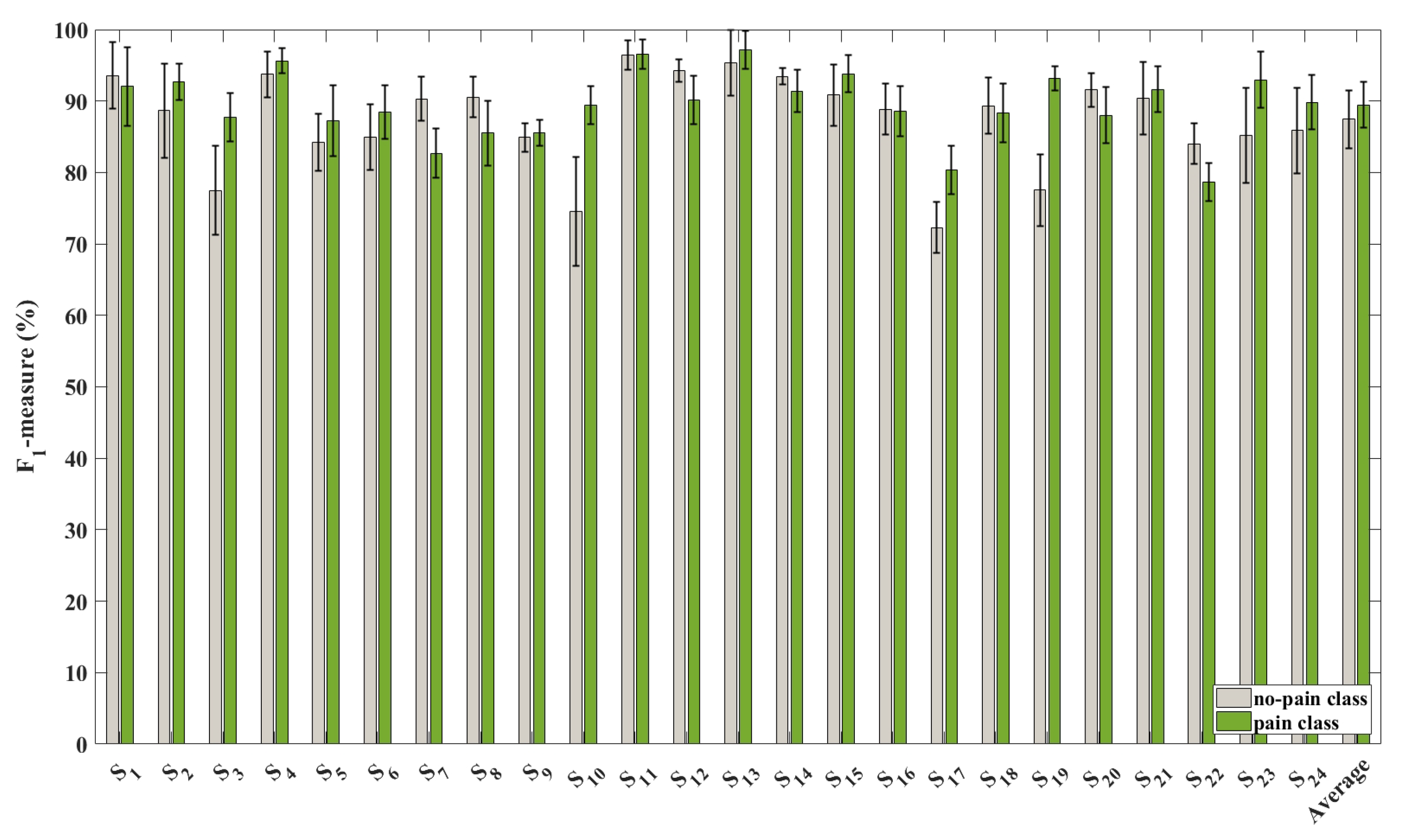
3.1.2. Results of the Channel Reduction Procedure

In this section, we present the results obtained for our proposed approach using the channel reduction procedure described in Section 2.7.

Table 2. The mean values of the average classification accuracies computed for each iteration of the channel reduction procedure over all subjects.

	Iterations of the Channel Reduction Procedure	Eliminated EEG Channel
		${\mathit{F}}_{\mathbf{7}}$	${\mathit{T}}_{\mathbf{7}}$	$\mathit{A}{\mathit{F}}_{\mathbf{3}}$	${\mathit{O}}_{\mathbf{1}}$	${\mathit{F}}_{\mathbf{4}}$	${\mathit{P}}_{\mathbf{7}}$	$\mathit{A}{\mathit{F}}_{\mathbf{4}}$	${\mathit{F}}_{\mathbf{8}}$	${\mathit{F}}_{\mathbf{3}}$	${\mathit{P}}_{\mathbf{8}}$	${\mathit{O}}_{\mathbf{2}}$	$\mathit{F}{\mathit{C}}_{\mathbf{5}}$	${\mathit{T}}_{\mathbf{8}}$	$\mathit{F}{\mathit{C}}_{\mathbf{6}}$
Average classification accuracy(%)	Iteration 1	83.76	83.53	83.69	83.82	84.08	83.59	83.89	83.78	84.11	84.15	83.93	84.23	83.59	84.33
	Iteration 2	83.19	82.98	82.96	83.55	83.29	83.27	83.42	82.82	83.24	83.20	83.75	83.60	83.76
	Iteration 3	81.83	82.18	82.13	82.43	82.52	82.40	82.11	82.07	82.40	82.61	82.55	82.63
	Iteration 4	81.60	81.62	81.13	82.38	81.98	81.92	81.99	82.04	81.98	82.30	82.57
	Iteration 5	80.81	81.22	80.88	81.30	81.37	81.32	81.51	81.44	81.59	81.72
	Iteration 6	80.54	80.37	79.11	80.43	80.68	80.68	80.57	80.84	81.08
	Iteration 7	78.98	79.63	78.26	79.71	79.66	79.64	79.75	79.98
	Iteration 8	77.58	78.27	77.75	78.26	78.10	78.24	78.72
	Iteration 9	75.70	76.27	76.29	76.31	76.46	76.96
	Iteration 10	74.20	74.86	74.29	74.75	75.34
	Iteration 11	71.41	71.69	72.06	72.23
	Iteration 12	68.32	69.20	71.01
	Iteration 13	65.08	65.90
	Iteration 14	65.90

shows the average classification accuracies computed over all subjects for each of the 14 iterations of the channel reduction procedure. Specifically, at the first iteration, eliminating the channel $F{C}_6$ provides an average classification accuracy of 84.33%, which is higher than the average classification accuracies obtained when any of the other 13 EEG channels is eliminated. In the second iteration, the additional elimination of the channel $T_8$ provides an average classification accuracy of 83.76%, which is higher than the average classification accuracies obtained when any of the remaining 12 EEG channels is eliminated. Moreover, in the subsequent iterations of the channel reduction procedure, the average classification accuracy is drastically decreasing after each iteration. Finally, at the last iteration, an average classification accuracy of 65.9% is achieved using the channel $F_7$.

Figure 4 indicates that the average classification accuracy obtained using all the EEG channels, which is equal to 84.6%, is higher than the average classification accuracies obtained after eliminating any of the EEG channels, where these accuracies are reported in Table 2. This can be attributed to several factors, including (1) the volume conductor effect [36], which describes the fact that the electrical potentials generated at a particular small region of the brain are spatially propagated to different regions of the brain. Consequently, these electrical potentials are recorded by the sparsely distributed electrodes on the scalp [6,23,36,37]. (2) The pain perception mechanism involves the activation of several regions of the brain, such as the frontal, prefrontal, temporal, parietal, and occipital regions [14,38,39,40]. Therefore, eliminating any EEG channel implies that the brain activities produced within the region covered by the eliminated channel might not be captured during the analysis. This can justify the observed decrease in the classification accuracies obtained during the channel reduction evaluation procedure. In light of the results presented in this section, we have utilized all the EEG channels to perform the feature-based evaluation procedure, which is presented in Section 3.2, and the performance comparison with the other previous approaches, which is described in Section 3.3.

3.2. Results of the Feature-Based Evaluation Procedure

In this section, we present the results obtained for our proposed approach using the feature reduction procedure described in Section 2.7.

Table 3. The mean values of the average classification accuracies computed for each iteration of the feature reduction procedure over all subjects.

	Iterations of the Feature Reduction Procedure	Eliminated Time-Frequency Feature
		$\mathit{T}{\mathit{F}}_{\mathbf{7}}$	$\mathit{T}{\mathit{F}}_{\mathbf{9}}$	$\mathit{T}{\mathit{F}}_{\mathbf{12}}$	$\mathit{T}{\mathit{F}}_{\mathbf{1}}$	$\mathit{T}{\mathit{F}}_{\mathbf{10}}$	$\mathit{T}{\mathit{F}}_{\mathbf{11}}$	$\mathit{T}{\mathit{F}}_{\mathbf{6}}$	$\mathit{T}{\mathit{F}}_{\mathbf{2}}$	$\mathit{T}{\mathit{F}}_{\mathbf{5}}$	$\mathit{T}{\mathit{F}}_{\mathbf{4}}$	$\mathit{T}{\mathit{F}}_{\mathbf{3}}$	$\mathit{T}{\mathit{F}}_{\mathbf{8}}$
Average classification accuracy(%)	Iteration 1	84.36	82.21	84.41	84.53	84.54	85.05	84.61	84.68	83.59	85.67	85.39	86.63
	Iteration 2	86.04	84.45	86.22	86.23	86.44	86.73	86.23	86.45	85.93	87.35	87.68
	Iteration 3	87.24	85.79	87.25	87.44	87.63	87.95	87.45	87.61	86.62	88.62
	Iteration 4	88.49	87.05	88.55	88.69	88.64	88.04	88.66	88.71	88.81
	Iteration 5	87.87	83.98	87.94	88.31	88.25	88.29	88.25	88.39
	Iteration 6	88.25	84.65	87.94	88.31	88.25	88.29	88.39
	Iteration 7	87.91	84.25	87.73	88.3	88.26	88.5
	Iteration 8	88.47	86.37	88.62	88.72	88.88
	Iteration 9	88.85	86.66	88.73	89.24
	Iteration 10	88.51	86.83	89.02
	Iteration 11	87.01	87.06
	Iteration 12	87.06

shows the average classification accuracies computed over all subjects for each of the 12 iterations of the feature reduction procedure. Specifically, at the first iteration, eliminating feature $T{F}_8$ provides an average classification accuracy of 86.63%, which is higher than the average classification accuracies obtained when any of the other 11 time-frequency features is eliminated. In the second iteration, the additional elimination of the feature $T{F}_3$ provides an average classification accuracy of 87.68, which is higher than the average classification accuracies obtained when eliminating any of the remaining 10 time-frequency features. Moreover, in the subsequent iterations of the feature reduction procedure, the average classification accuracy keeps increasing until the 9th iteration, at which the average classification accuracy achieved using the time-frequency features $T{F}_7$, $T{F}_9$, and $T{F}_{12}$ is 89.24%. In the consecutive iterations, the average classification accuracy starts to decrease after each iteration. Finally, at the last iteration, an average classification accuracy of 87.06% is achieved using the time-frequency feature $T{F}_7$.

Table 3 shows that the average classification accuracy obtained using only the $T{F}_7$, $T{F}_9$, and $T{F}_{12}$ features, which is equal to 89.24%, is higher that the average classification accuracy obtained using all the CWD-based time-frequency features, which is equal to 84.6%, as shown in Figure 4. In addition, the results presented in Table 3 suggest that the best classification accuracy can be obtained by eliminating all the features except $T{F}_7$, $T{F}_9$, and $T{F}_{12}$. This can be attributed to two factors: (1) The physical interpretation of the quantities measured by each of these three features. In particular, the feature $T{F}_7$, which is the root mean square of the CWD, measures the strength of the signal energy in the time-frequency domain [6,7,17,23]. The feature $T{F}_9$, which is the time-frequency flatness of the CWD, measures the rate of change of the signal energy in the time-frequency domain [6,7,17,23]. Finally, the feature $T{F}_{12}$, which is the time-frequency energy of the CWD, measures the concentration of the signal energy in the time-frequency domain [6,7,17,23]. In fact, further analysis is needed to explore the correlation between the energy characteristics of the EEG signals and the capability of detecting pain. (2) Recently, researchers have shown that during pain there are several neural oscillations that are associated with different frequency bands and are generated across various regions of the brain [10,41]. Therefore, using the computed values of the aforementioned three features enables capturing the time-varying spectral oscillations encapsulated within EEG segments, where such time-varying spectral oscillations can contribute to the task of differentiating between the no-pain and pain classes.

It is worth noting that the use of the time-frequency features $T{F}_9$ and $T{F}_{12}$ in different EEG-based classification problems, such as decoding human emotions [23] and motor imagery tasks [6], has yielded a higher classification accuracies compared with the other time-frequency features. This implies the capability of these time-frequency features to capture the nonstationary and nonlinear characteristics of the EEG signals. This in turn suggests the possibility of employing these features in the design process of several EEG-based classification problems [23].

Figure 6 shows the classification accuracy values and the corresponding standard deviations obtained for each subject using the features $T{F}_7$, $T{F}_9$, and $T{F}_{12}$. In particular, the average classification accuracy values computed for the 24 subjects are between 81.9%, which was obtained for $S_{22}$, and 96.5%, which was obtained for $S_{13}$. Moreover, the average classification accuracy value obtained for each subject is significantly higher than the random classification rate, which is defined as the reciprocal of the number of classes, and equal to 50% (the red dashed line in Figure 6). The average ± standard deviation classification accuracy value achieved in distinguishing between the no-pain and pain classes using the features $T{F}_7$, $T{F}_9$, and $T{F}_{12}$, which is computed over all 24 subjects, is equal to $89.2\%\pm 3.2\%$. The average ± standard deviations of $F_1-$ measure values computed for the no-pain and pain classes per each subject using the features $T{F}_7$, $T{F}_9$, and $T{F}_{12}$ are provided in Figure 7. In particular, the average ± standard deviation of $F_1-$ measure values computed for the no-pain and pain classes over all subjects are $87.4\%\pm 4.1\%$ and $89.5\%\pm 3.3\%$, respectively. The results presented in Figure 6 and Figure 7, which are obtained using the features $T{F}_7$, $T{F}_9$, and $T{F}_{12}$, outperform the results obtained using all the EEG channels and all the features, which are shown in Figure 4 and Figure 5.

3.3. Comparison with Other Approaches

In this section, we compare the classification results obtained using our proposed CWD-based time-frequency features with the classification results obtained using the features presented in the studies [8] and [9], respectively, as described in Section 2.7.

Table 4. Comparison with other approaches.

Approach	Features	Accuracy(%) ± Standard Deviation (%)
Nir et al. [8]	Peak alpha frequency	81.1 ± 5.2
Panavaranan and Wongsawat [9]	Normalize PSD of the alpha and beta frequency bands	75.6 ± 8.7
This work	CWD-based time-frequency features	89.2 ± 3.2

provides the average ± standard deviations classification accuracies computed over all 24 subjects for the methods presented in the studies [8] and [9]. Specifically, using the feature presented by Nir et al. [8], the average ± standard deviation classification accuracy value achieved in distinguishing between the no-pain and pain classes, which is computed over all 24 subjects, is equal to $81.1\%$ ± $5.2\%$. Similarly, using the features presented by Panavaranan and Wongsawat [9], the average ± standard deviation classification accuracy value achieved in distinguishing between the no-pain and pain classes, which is computed over all 24 subjects, is equal to $75.6\%$ ± $8.7\%$. The results presented in Table 4 indicate that the classification accuracy obtained using our proposed CWD-based time-frequency features outperforms the classification accuracies obtained using the features described by the authors of [8,9]. This suggests the feasibility of employing our proposed CWD-based time-frequency features to successfully distinguish between the EEG segments associated with the no-pain and pain classes.

3.4. Limitations and Future Work

In spite of the promising results achieved using our proposed CWD-based approach in distinguishing between the no-pain and pain classes, we are planning to investigate several research directions that can enhance the accuracy and applicability of our proposed pain detection approach. Specifically, we are intending to explore four future research directions: (1) Recently, few researchers have successfully utilized deep learning techniques to analyze the time-frequency maps constructed for the EEG signals [42,43]. In this regard, we intend to investigate the possibility of employing deep learning techniques, such as convolutional neural networks (CNN), to extract data-driven deep features from the constructed CWD-based TFR of the EEG signals that can enhance the accuracy of pain detection. (2) The subjective nature of pain, which introduces a significant intra- and intersubject variations in the responses of subjects to external painful stimuli, along with the nonstationary nature of the EEG signals increase the necessity to acquire a large-scale and balanced database that can be used to design a subject-independent pain detection system. In addition, the results obtained based on physiological signals, such as the EEG signals, that are acquired under well-controlled lab conditions may overestimate the results that can be achieved in real-world applications, in which minimally controlled acquisition conditions are maintained. In light of this, we plan to record a large-scale database under realistic recording conditions to assess the capability of our proposed CWD-based pain detection approach to support real-world applications. (3) We also plan to extend our work by utilizing the extracted time-frequency features to estimate the pain level that a patient is feeling. Such an extension can enhance the ability of the caregivers to characterize and mange clinical pain for patients who are not capable to verbally express their feelings, such as infants. (4) We plan to extend the analyses performed in the current study from subject-specific analyses to subject-independent analyses. The subject-independent analyses can measure the ability of our proposed CWD-based pain detection approach to detect pain for new subjects that were not included in the training set, which can be useful for several real-world applications.

4. Conclusions

In this paper, we have proposed an EEG-based approach for detecting tonic cold pain. The proposed approach utilizes a set of time-frequency features that are extracted from the constructed CWD-based TFR of the EEG signals to train a SVM classifier that can accurately distinguish between the no-pain and pain states. The results presented in this work indicate that the EEG signals comprise rich information that can be used to understand the pain perception mechanism. In addition, the results suggest the feasibility of using the CWD to analyze the EEG signals and extract quantitative time-frequency features that are capable of distinguishing between different finger movements.

References

1. Williamson, A.; Hoggart, B. Pain: A review of three commonly used pain rating scales. J. Clin. Nurs. 2005, 14, 798–804. [Google Scholar] [CrossRef] [PubMed]
2. Herr, K.; Coyne, P.J.; McCaffery, M.; Manworren, R.; Merkel, S. Pain assessment in the patient unable to self-report: Position statement with clinical practice recommendations. Pain Manag. Nurs. 2011, 12, 230–250. [Google Scholar] [CrossRef] [PubMed]
3. Lamothe, M.; Roy, J.S.; Bouffard, J.; Gagné, M.; Bouyer, L.J.; Mercier, C. Effect of tonic pain on motor acquisition and retention while learning to reach in a force field. PLoS ONE 2014, 9, e99159. [Google Scholar] [CrossRef] [PubMed]
4. Sinke, C.; Schmidt, K.; Forkmann, K.; Bingel, U. Phasic and tonic pain differentially impact the interruptive function of pain. PLoS ONE 2015, 10, e0118363. [Google Scholar] [CrossRef] [PubMed]
5. Nicolas-Alonso, L.F.; Gomez-Gil, J. Brain computer interfaces, a review. Sensors 2012, 12, 1211–1279. [Google Scholar] [CrossRef] [PubMed]
6. Alazrai, R.; Alwanni, H.; Baslan, Y.; Alnuman, N.; Daoud, M.I. EEG-Based Brain-Computer Interface for Decoding Motor Imagery Tasks within the Same Hand Using Choi–Williams Time-Frequency Distribution. Sensors 2017, 17, 1937. [Google Scholar] [CrossRef] [PubMed]
7. Alazrai, R.; Alwanni, H.; Daoud, M.I. EEG-based BCI system for decoding finger movements within the same hand. Neurosci. Lett. 2019, 698, 113–120. [Google Scholar] [CrossRef] [PubMed]
8. Nir, R.R.; Sinai, A.; Raz, E.; Sprecher, E.; Yarnitsky, D. Pain assessment by continuous EEG: Association between subjective perception of tonic pain and peak frequency of alpha oscillations during stimulation and at rest. Brain Res. 2010, 1344, 77–86. [Google Scholar] [CrossRef] [PubMed]
9. Panavaranan, P.; Wongsawat, Y. EEG-based pain estimation via fuzzy logic and polynomial kernel support vector machine. In Proceedings of the 6th IEEE Biomedical Engineering International Conference, Amphur Muang, Thailand, 23–25 October 2013; pp. 1–4. [Google Scholar]
10. Shao, S.; Shen, K.; Yu, K.; Wilder-Smith, E.P.; Li, X. Frequency-domain EEG source analysis for acute tonic cold pain perception. Clin. Neurophysiol. 2012, 123, 2042–2049. [Google Scholar] [CrossRef] [PubMed]
11. Vatankhah, M.; Toliyat, A. Pain Level Measurement Using Discrete Wavelet Transform. Int. J. Eng. Technol. 2016, 8, 380–384. [Google Scholar] [CrossRef] [Green Version]
12. Akansu, A.N.; Haddad, P.A.; Haddad, R.A.; Haddad, P.R. Multiresolution Signal Decomposition: Transforms, Subbands, and Wavelets; Academic Press: Cambridge, MA, USA, 2001. [Google Scholar]
13. Mallat, S. A Wavelet Tour of Signal Processing: The Sparse Way; Academic Press: Cambridge, MA, USA, 2008. [Google Scholar]
14. Hadjileontiadis, L.J. EEG-Based Tonic Cold Pain Characterization Using Wavelet Higher Order Spectral Features. IEEE Trans. Biomed. Eng. 2015, 62, 1981–1991. [Google Scholar] [CrossRef] [PubMed]
15. Alazrai, R.; Aburub, S.; Fallouh, F.; Daoud, M.I. EEG-based BCI system for classifying motor imagery tasks of the same hand using empirical mode decomposition. In Proceedings of the 10th IEEE International Conference on Electrical and Electronics Engineering (ELECO), Bursa, Turkey, 30 November–2 December 2017; pp. 615–619. [Google Scholar]
16. Toole, J.M.O. Discrete Quadratic Time-Frequency Distributions: Definition, Computation, and a Newborn Electroencephalogram Application. Ph.D. Thesis, School of Medicine, The University of Queensland, Brisbane, Australia, 2009. [Google Scholar]
17. Boashash, B. Time-fRequency Signal Analysis and Processing: A Comprehensive Reference; Academic Press: Cambridge, MA, USA, 2015. [Google Scholar]
18. Boashash, B.; Azemi, G.; O’Toole, J.M. Time-Frequency Processing of Nonstationary Signals: Advanced TFD Design to Aid Diagnosis with Highlights from Medical Applications. IEEE Signal Process. Mag. 2013, 30, 108–119. [Google Scholar] [CrossRef]
19. Boashash, B.; Ouelha, S. Automatic signal abnormality detection using time-frequency features and machine learning: A newborn EEG seizure case study. Knowl.-Based Syst. 2016, 106, 38–50. [Google Scholar] [CrossRef]
20. Dowman, R.; Rissacher, D.; Schuckers, S. EEG indices of tonic pain-related activity in the somatosensory cortices. Clin. Neurophysiol. 2008, 119, 1201–1212. [Google Scholar] [CrossRef] [PubMed] [Green Version]
21. Delorme, A.; Makeig, S. EEGLAB: An open source toolbox for analysis of single-trial EEG dynamics including independent component analysis. J. Neurosci. Methods 2004, 134, 9–21. [Google Scholar] [CrossRef] [PubMed]
22. Gómez-Herrero, G.; De Clercq, W.; Anwar, H.; Kara, O.; Egiazarian, K.; Van Huffel, S.; Van Paesschen, W. Automatic removal of ocular artifacts in the EEG without an EOG reference channel. In Proceedings of the IEEE 7th Nordic Signal Processing Symposium, Rejkjavik, Iceland, 7–9 June 2006; pp. 130–133. [Google Scholar]
23. Alazrai, R.; Homoud, R.; Alwanni, H.; Daoud, M.I. EEG-Based Emotion Recognition Using Quadratic Time-Frequency Distribution. Sensors 2018, 18, 2739. [Google Scholar] [CrossRef] [PubMed]
24. Castiglioni, P. Choi–Williams Distribution. In Encyclopedia of Biostatistics; John Wiley & Sons, Ltd.: Hoboken, NJ, USA, 2005. [Google Scholar]
25. Alazrai, R.; Momani, M.; Khudair, H.A.; Daoud, M.I. EEG-based tonic cold pain recognition system using wavelet transform. Neural Comput. Appl. 2017. [Google Scholar] [CrossRef]
26. Choi, H.I.; Williams, W.J. Improved time-frequency representation of multicomponent signals using exponential kernels. IEEE Trans. Acoust. Speech Signal Process. 1989, 37, 862–871. [Google Scholar] [CrossRef]
27. Hahn, S.L. Hilbert Transforms in Signal Processing; Artech House Boston: Norwood, MA, USA, 1996; Volume 2. [Google Scholar]
28. Swami, A.; Mendel, J.; Nikias, C. Higher-Order Spectra Analysis (HOSA) Toolbox. Version 2.0. 2000. Available online: http://www.mathworks.com/matlabcentral/fileexchange/3013 (accessed on 30 June 2019).
29. Chang, C.C.; Lin, C.J. LIBSVM: A library for support vector machines. ACM Trans. Intell. Syst. Technol. 2011, 2, 27. [Google Scholar] [CrossRef]
30. Hsu, C.W.; Chang, C.C.; Lin, C.J. A Practical Guide to Support Vector Classification; Technical Report; Department of Computer Science, National Taiwan University: Taipei, Taiwan, 2003. [Google Scholar]
31. Al-Timemy, A.H.; Bugmann, G.; Escudero, J.; Outram, N. Classification of Finger Movements for the Dexterous Hand Prosthesis Control With Surface Electromyography. IEEE J. Biomed. Health Inform. 2013, 17, 608–618. [Google Scholar] [CrossRef] [PubMed]
32. Goge, A.; Chan, A. Investigating Classification Parameters for Continuous Myoelectrically Controlled Prostheses; Canadian Medical and Biological Engineering Society: Ottawa, ON, Canada, 2005; Volume 28. [Google Scholar]
33. Li, G.; Schultz, A.E.; Kuiken, T.A. Quantifying Pattern Recognition—Based Myoelectric Control of Multifunctional Transradial Prostheses. IEEE Trans. Neural Syst. Rehabil. Eng. 2010, 18, 185–192. [Google Scholar] [PubMed]
34. Li, G.; Kuiken, T.A. EMG pattern recognition control of multifunctional prostheses by transradial amputees. In Proceedings of the 2009 Annual International Conference of the IEEE Engineering in Medicine and Biology Society, Minneapolis, MN, USA, 3–6 September 2009; pp. 6914–6917. [Google Scholar]
35. Han, J.; Pei, J.; Kamber, M. Data Mining: Concepts and Techniques; Elsevier: Amsterdam, The Netherlands, 2011. [Google Scholar]
36. Van den Broek, S.P.; Reinders, F.; Donderwinkel, M.; Peters, M. Volume conduction effects in EEG and MEG. Electroencephalogr. Clin. Neurophysiol. 1998, 106, 522–534. [Google Scholar] [CrossRef]
37. Liao, K.; Xiao, R.; Gonzalez, J.; Ding, L. Decoding individual finger movements from one hand using human EEG signals. PLoS ONE 2014, 9, e85192. [Google Scholar] [CrossRef] [PubMed]
38. Aftanas, L.; Reva, N.; Varlamov, A.; Pavlov, S.; Makhnev, V. Analysis of evoked EEG synchronization and desynchronization in conditions of emotional activation in humans: Temporal and topographic characteristics. Neurosci. Behav. Physiol. 2004, 34, 859–867. [Google Scholar] [CrossRef] [PubMed]
39. Mohammadi, Z.; Frounchi, J.; Amiri, M. Wavelet-based emotion recognition system using EEG signal. Neural Comput. Appl. 2017, 28, 1985–1990. [Google Scholar] [CrossRef]
40. Penfield, W.; Rasmussen, T.; Erickson, T. The Cerebral Cortex of Man, a Clinical Study of Localization of Function. Am. J. Phys. Med. Rehabil. 1954, 33, 126. [Google Scholar]
41. Borckardt, J.J.; Romagnuolo, J.; Reeves, S.T.; Madan, A.; Frohman, H.; Beam, W.; George, M.S. Feasibility, safety, and effectiveness of transcranial direct current stimulation for decreasing post-ERCP pain: A randomized, sham-controlled, pilot study. Gastrointest. Endosc. 2011, 73, 1158–1164. [Google Scholar] [CrossRef] [PubMed]
42. Morabito, F.C.; Campolo, M.; Mammone, N.; Versaci, M.; Franceschetti, S.; Tagliavini, F.; Sofia, V.; Fatuzzo, D.; Gambardella, A.; Labate, A.; et al. Deep learning representation from electroencephalography of early-stage Creutzfeldt-Jakob disease and features for differentiation from rapidly progressive dementia. Int. J. Neural Syst. 2017, 27, 1650039. [Google Scholar] [CrossRef] [PubMed]
43. Alazrai, R.; Abuhijleh, M.; Alwanni, H.; Daoud, M.I. A Deep Learning Framework for Decoding Motor Imagery Tasks of the Same Hand using EEG Signals. IEEE Access 2019, 7, 109612–109627. [Google Scholar] [CrossRef]
Figure 1. Timing diagram of the experimental procedure during each trial. T represents the length of the trial.
Applsci 09 03433 g001
Figure 2. The positions of the electroencephalography (EEG) electrodes of the Emotiv neuroheadset arranged on the scalp according to the international 10–20-electrode placement system.
Applsci 09 03433 g002
Figure 3. Graphical illustration of the constructed Choi–Williams distribution (CWD)-based time-frequency representation (TFR) for two different EEG segments that were extracted from the 3rd trial of subject 11. (a) An example EEG segment of the no-pain class. (b) The CWD-based TFR constructed for the no-pain EEG segment presented in Figure 3a. (c) An example EEG segment of the pain class. (d) The CWD-based TFR constructed for the pain EEG segment presented in Figure 3c.
Applsci 09 03433 g003
Figure 4. The average classification accuracy values computed for each subject over the ten train–test repetitions of the employed cross-validation procedure. The black vertical lines represent the standard deviations of the classification accuracy and the red dashed line represents the random classification rate. The last column represents the mean value of the average classification accuracies computed over the 24 subjects.
Applsci 09 03433 g004
Figure 5. The average F 1 - measure accuracy values computed for the no-pain and pain classes per each subject over the ten train–test repetitions of the employed cross-validation procedure. The black vertical lines represent the standard deviations of the classification accuracy and the red dashed line represents the random classification rate. The last column represents the mean value of the average F 1 - measure values of the no-pain and pain classes computed over the 24 subjects.
Applsci 09 03433 g005
Figure 6. The average classification accuracy values computed for each subject over the ten train–test repetitions of the employed cross-validation procedure using the features T F 7 , T F 9 , and T F 12 . The black vertical lines represent the standard deviations of the classification accuracy and the red dashed line represents the random classification rate. The last column represents the mean value of the average classification accuracies computed over the 24 subjects.
Applsci 09 03433 g006
Figure 7. The average F 1 - measure accuracy values computed for the no-pain and pain classes per each subject over the ten train–test repetitions of the employed cross-validation procedure using the features T F 7 , T F 9 , and T F 12 . The black vertical lines represent the standard deviations of the classification accuracy and the red dashed line represents the random classification rate. The last column represents the mean value of the average F 1 - measure values of the no-pain and pain classes computed over the 24 subjects.
Applsci 09 03433 g007