Seismic Control of SDOF Systems with Nonlinear Eddy Current Dampers

Featured Application

This work deals with the dynamic response calculation and energy dissipation analysis of a linear elastic single-degree-of-freedom (SDOF) system with a supplemental nonlinear eddy current damper (ECD) subjected to base excitation, in preparation for optimum design and performance evaluation for structural vibration control with ECDs.

Abstract

The nonlinear model and energy dissipation of a rotary axial eddy current damper (ECD) and the dynamic responses to harmonic and seismic base excitations of a linear elastic SDOF system with the nonlinear ECD (SDOF-ECD) are investigated. Firstly, the nonlinear force-velocity relationship of the ECD is studied using finite element simulation, experimental testing and mathematical model fitting. Secondly, the energy dissipated by the nonlinear ECD under a cycle of harmonic motion is derived analytically and its optimal critical velocity is determined such that the energy dissipation is maximized. Finally, the responses of the SDOF-ECDs subjected to harmonic and seismic base excitations are calculated using numerical algorithm, where the displacement and acceleration control performance and the energy dissipation capacity of the ECD are compared with those of the conventional fluid viscous dampers (FVDs). The results indicate that the seismic control performance of ECDs outperforms that of FVDs in most cases and it is anticipated that the ECDs can be used as good alternative devices to conventional FVDs for seismic control applications.

1. Introduction

Structural vibration control has been widely applied in civil engineering, such as wind-induced vibration reduction and seismic protection of high-rise buildings [1,2,3,4,5], seismic response mitigation of long span bridges [6,7,8], human-induced vibration control of footbridges and floor decks [9,10], vibration control of stay cables [11,12,13], vibration control of wind turbines [14,15,16] and vibration control of marine structures [16,17], etc. Energy dissipation devices, such as fluid viscous dampers (FVDs) [6,18], magnetorheological (MR) dampers [7,11,12], pounding dampers [17,19,20,21] and electromagnetic dampers [2,9,22,23,24,25], can suppress structural vibration effectively. In recent years, an innovative control device named eddy current damper (ECD) has gained more and more attention in the field of structural vibration control. The eddy current damping is a kind of magnetic damping, which is contactless between the movable members. Therefore, wear and fatigue are minimized in the ECDs, minimum maintenance is required and lifetime is maximized, gently outperforming that of contact-type dampers. Compared to conventional FVDs, there is no working fluid and no fluid degradation and leakage problems exist in the ECDs. The ECDs can be made tube-like and produce an axial force [26], or coupled with a ball screw to form a rotary axial eddy current damper [27]. The eddy current damping unit can be also integrated with a mass and a spring to form an eddy current tuned mass damper (EC-TMD) [2,22].

In its simplest form, an ECD device consists of a conductive plate and a pair of magnets. When the conductive plate moves through a magnetic field, the movement induces an eddy current in the conductive plate. The interaction of the eddy currents and the applied magnetic field induces a drag force that resists the relative motion between the conductive plate and the magnets. The drag force is also called the eddy current damping force. However, the energy dissipation density of such an eddy current damping system is usually very low, and this disadvantage does restrict its industrial applications [26]. In recent years, significant improvements have been made by either enhancing magnetic strength or increasing the speed of relative movement. For example, the use of back irons in the ECDs is shown to increase the damping coefficients by a factor of up to five [22]. The relative speed between the conductive plate and magnets can be amplified using a ball screw [27] or a linear magnetic gear [28]. A ball screw can transform low speed linear motion into high speed rotary motion and a linear magnetic gear can amplify the linear speed by several times.

For the ECDs without velocity amplification, the relative velocity between the conductive plate and magnets is not very high if the external excitations are in the low frequency band. In such cases, the constitutive behavior of eddy current damping is linear for the relationship between the damping force and relative velocity [22]. When the external excitations are in very high frequency band such as earthquakes and impact loads, or the ECDs are enhanced with amplification mechanisms such as the ball screw or magnetic gear, the relative velocity between the conductive plate and magnets becomes much higher. In such cases, the constitutive behavior of eddy current damping is nonlinear due to the influence of the reaction field of the eddy current in the conductive plate [29].

It is common in both design and retrofit of structures to approximate the real multi-degree-of-freedom (MDOF) system with an equivalent single-degree-of-freedom (SDOF) system such that the latter represents the most relevant characteristics of the former for a particular motion mode. In this way, any preliminary attempt to design a supplemental damping system for a structure can be simplified allowing the designer to use an equivalent SDOF model instead. In view of the nonlinear properties of ECDs, the governing equation for an SDOF-ECD system becomes nonlinear, which is difficult to calculate the system response analytically. On the other hand, as structural engineers are most familiar with classical viscous damping, it is essential to compare the performance of ECDs with FVDs, which are nonlinear in nature as well.

This investigation aims to demonstrate how nonlinear ECDs affect the dynamic responses of SDOF systems and evaluate the seismic control performance compared with FVDs. Presented first are the nonlinear characteristics of a rotary axial ECD, where we demonstrate that its force-velocity relationship can be characterized by the Wouterse’s model [29]. Secondly, the energy dissipation capacity of the nonlinear ECD is derived analytically when subjected to harmonic motion and its optimal critical velocity for energy dissipation are obtained, where its energy dissipation characteristics are compared with FVDs. Thirdly, steady-state responses of the SDOF-ECD systems under harmonic excitations are calculated using numerical simulations, their displacement and acceleration responses are compared with those of the SDOF-FVD systems. Fourthly, the seismic response control performance and energy dissipation capacity of the SDOF-ECD systems under real earthquakes are analyzed and compared with the SDOF-FVD systems. Some conclusion remarks are drawn in the final part.

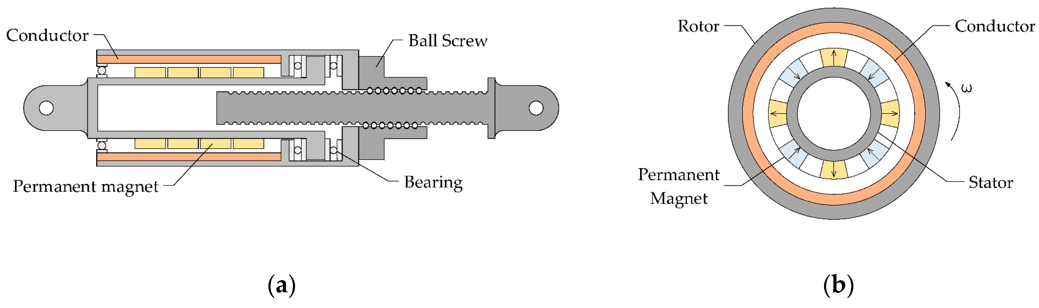
2. Nonlinear Constitutive Behavior of an Eddy Current Damper

Generally speaking, the mathematical models for supplemental damping devices are quite complicated. The most widely used energy dispassion devices are FVDs. Experimental evidence [30] reveals that the constitutive behavior of FVDs for the force-velocity relationship can be described by a fractional velocity power law as follows

$$F_{FVD}=c_d{v}^{\alpha }$$

(1)

where c_d is a damping coefficient, α is a velocity exponent, and v is the relative velocity between two ends of the damper. The exponent α is responsible for the nonlinear damping of FVDs and depends upon the hydraulic circuit employed. Typically, α ranges from 0.35 to 1.00 for seismic mitigation applications [18].

For eddy current dampers, the constitutive behavior models for the force-velocity relationship are quite different from those of FVDs. When the relative speed is low, the force-velocity relationship is linear, and it becomes nonlinear when the relative speed goes higher. In 2014, Chen proposed a rotary axial eddy current damper [27], in which a ball screw is employed to amplify the relative speed by transforming the linear motion to a rotary motion. The longitudinal and transverse cross sections of the rotary axial ECD are shown in Figure 1. The damper comprises two main components, i.e., a ball screw assembly and an eddy current damping generator. The ball screw assembly comprises a ball screw drive pair, a stator and a rotor respectively made of magnetic conductive materials. The eddy current damping generators comprise permanent magnets (PMs) and conductive plate, which are arranged on the stator and the outer rotor, respectively.

In order to characterize the constitutive behavior for the force-velocity relationship of such a new kind of rotary axial ECDs, both finite element simulations and full scale laboratory experiments are conducted. It is found that the nonlinear constitutive behavior of the force-velocity relationship can be well characterized by the Wouterse’s model [29] as follows

$$F_{ECD}=F_{max}\frac{2}{\frac{v}{v_{cr}} + \frac{v_{cr}}{v}}$$

(2)

where $F_{max}$ is the maximum damping force, and $v_{cr}$ is the critical relative velocity when the damping force reaches the maximum value. It should be noted that $F_{max}$ and $v_{cr}$ are dependent on the design parameters of the damper, such as the remanence of the PMs, the thickness of the conductive plate and the air gap, etc.. The measured data points from full scale laboratory experiments, the finite element method (FEM) simulation curve and the fitting curve by the Wouterse’s model are plotted in Figure 2. The designed $v_{cr}$ for the tested damper is 0.259 m/s. It can be seen that the Wouterse’s model can depict the nonlinear constitutive behavior of such kind of ECDs very well. In the following, the energy dissipation and response mitigation analysis are all based on this model. From Figure 2, it can be seen that the eddy current damping force is approximately linearly proportional to the relative velocity in the low speed region, gradually increasing with decreasing slope when the relative velocity becomes higher, reaching a maximum value at the critical speed, and then decreasing for much higher speeds. Although the experimental data do not cover the decreasing stage due to the limitations of the testing machine, the finite element simulation curve has revealed the characteristic of damping force decreasing at much higher speeds. This characteristic of eddy current damping has also been reported in other literatures [29,31,32,33]. This unique characteristic can protect the damper and the connection part between the damper and structure from damage when an over-load is exerted on the damper. For example, when a huge impact load is exerted on the damper, the damping force will decrease at much higher speeds for ECDs, but for conventional FVDs without unloading mechanisms, the damping force will go up again and consequently the damper and the connection part will be damaged due to relatively great local stress.

3. Energy Dissipation Analysis

3.1. Energy Dissipation Capacity Under Harmonic Motion

Compared with FVDs, the ECDs have quite different constitutive behavior for the force-velocity relationship. In view of these differences, we have to analyze their energy dissipation capacities as compared with FVDs. The dampers are assumed to be subjected to harmonic motion $u=u_0\sin (\omega t)$. Here, we assumed the maximum damping force $F_{max}$ in the ECD is the same as the maximum damping force in the FVD under the same harmonic motion. It should be noted that the maximum damping force of ECDs will occur at the critical velocity which is not necessary the same as the maximum velocity, while the maximum damping force of FVDs happens at the maximum velocity. Under the conditions of the same harmonic motion and the same maximum damping force, we will compare the energy dissipation capacities of ECDs and FVDs.

For FVDs which is governed by Equation (1), the energy dissipated by the damper during a cycle of harmonic motion $u=u_0\sin (\omega t)$ is [18]

$$E_{\mathrm{FVD}}=4{{\displaystyle \int }}_0^{u_0}{F}_{\mathrm{FVD}}\mathrm{d}u=\frac{2C_d\sqrt{\pi }{u}_0^{\alpha + 1}{\omega }^{\alpha }\Gamma (\frac{\alpha }{2} + 1)}{\Gamma (\frac{\alpha +3}{2})}$$

(3)

where $\Gamma (x)$ is the gamma function.

For ECDs which is governed by Equation (2), the energy dissipated by the damper during a cycle of the same harmonic motion $u=u_0\sin (\omega t)$ is

$$E_{\mathrm{ECD}}=4{{\displaystyle \int }}_0^{u_0}\frac{2F_{max}}{\frac{v}{v_{cr}} + \frac{v_{cr}}{v}}\mathrm{d}u=\frac{4v_{cr}{F}_{max}\pi }{\omega }(1-\frac{v_{cr}}{\sqrt{v_{cr}^2 + u_0^2{\omega }^2}})$$

(4)

The detailed formula derivation is shown in Appendix A. It can be seen that $E_{\mathrm{ECD}}$ is a function of $v_{cr}$ when $F_{max}$, $u_0$ and $\omega$ are specified. In the following section, we will derive the optimal $v_{cr}$ when the energy dissipation capacity $E_{\mathrm{ECD}}$ is maximized.

3.2. Optimal Critical Velocity Under Harmonic Motion

In order to determine the maximum energy dissipation capacity of ECDs, here we use FVDs as the reference, and take the dimensionless energy ratio $E_{\mathrm{ECD}}/E_{\mathrm{FVD}}$ as the objective function. It should be noted that the maximum velocity of the harmonic motion $u=u_0\sin (\omega t)$ is $u_0\omega$. Here, we take the dimensionless velocity ratio $X=v_{cr}/u_0\omega$ as the dependent variable. From the governing Equation (1) of FVDs, the maximum damping force is

$$F_{max}=c_d{(u_0\omega )}^{\alpha }$$

(5)

From Equations (3)–(5), the dimensionless energy ratio can be obtained as

$$\frac{E_{\mathrm{ECD}}}{E_{\mathrm{FVD}}}=\frac{2\sqrt{\pi }\Gamma (\frac{\alpha + 3}{2})}{\Gamma (\frac{\alpha }{2} + 1)}X(1-\frac{1}{\sqrt{1 + \frac{1}{X^2}}})$$

(6)

Through observing the mathematical structure of Equation (6), it can be seen that the term $\frac{2\sqrt{\mathsf{\pi }}\mathsf{\Gamma }(\frac{\mathsf{\alpha }+3}{2})}{\mathsf{\Gamma }(\frac{\mathsf{\alpha }}{2}+1)}$ is determined by the velocity exponent α of the FVDs, and the other term $\mathrm{X}(1-\frac{1}{\sqrt{1+\frac{1}{X^2}}})$ is determined by the dimensionless velocity ratio X of ECDs.

For a certain design of FVD, the velocity exponent α is specified. Here, we use the dimensionless velocity ratio X as the dependent variable to find an optimal design of ECD such that the energy dissipation of ECD is maximized as compared to that of the FVD. Let’s denote $Y=X(1- \frac{1}{\sqrt{1 + \frac{1}{X^2}}})$, and take its derivatives, we can know that when $X=\sqrt{\frac{1}{2}(-1+\sqrt{5})}\approx 0.786$, the energy dissipation ratio $\frac{E_{\mathrm{ECD}}}{E_{\mathrm{FVD}}}$ reaches the maximum (See Appendix B). It can be seen that when the ratio of the critical velocity to the maximum velocity is 0.786, the energy dissipation capacity of ECD reaches its maximum. It should be noted that the energy dissipation ratio is also dependent on the velocity exponent α of FVDs. The energy dissipation ratio versus the velocity ratio is plotted in Figure 3.

From Figure 3, it can be seen that it always can find a better design of ECD when the velocity exponent α of FVD is larger than 0.2 such that the energy dissipation capacity of ECD is larger than that of FVD under the same harmonic motion. As we know, the velocity exponent α of FVDs ranges from 0.35 to one for seismic applications, and therefore the ECDs can be used as good alternative devices for seismic response mitigation. It is particularly worth pointing out that the critical velocity corresponding to the maximum damping force is not the designed maximum velocity of the damper and the damping force will fall down when the velocity is larger than the critical velocity. This unique characteristic guarantees that the failure risk of dampers and mounting supports can be reduced in case of an over-limit earthquake.

4. SDOF Systems with Nonlinear Eddy Current Dampers

In order to further analyze the response mitigation performance and energy dissipation capacity of nonlinear ECDs, we consider a linear elastic SDOF system supplemented with an ECD. The governing equation of the SDOF-ECD coupling system, the steady state response to the harmonic excitation, and the dynamic response and energy dissipation to seismic excitation are analyzed in detail in the following sessions.

4.1. Equations of Motion and System Paramerts

The schematic model of the SDOF system with a supplemental damper subjected to ground motion is shown in Figure 4. The equation governing the motion of the SDOF system with mass m, elastic stiffness k, linear viscous damping coefficient c, and a nonlinear FVD subjected to ground acceleration ${\ddot{u}}_g(t)$ is

$$m\ddot{u}+c\dot{u}+ku+c_d{\dot{u}}^{\alpha }=-m{\ddot{u}}_g$$

(7)

while for the SDOF-ECD coupling system, the equation governing the motion is

$$m\ddot{u}+c\dot{u}+ku+F_{max}\frac{2}{\frac{\dot{u}}{{\dot{u}}_{cr}} + \frac{{\dot{u}}_{cr}}{\dot{u}}}=-m{\ddot{u}}_g$$

(8)

The system parameters are selected from a longitudinal motion mode of a long span suspension bridge as follows: The mass $m=1.4\times {10}^7 \mathrm{kg}$; the natural frequency $f=0.124 \mathrm{Hz}$; the structural damping ratio $\zeta =0.02$; the peak ground acceleration ${\ddot{u}}_{go}=1.5247 \mathrm{m}/{\mathrm{s}}^2$. In order to compare the response mitigation performance of ECDs and FVDs, here we set the damping coefficient of the FVD $c_d=1.2\times {10}^7\mathrm{N}/{(\mathrm{m}/\mathrm{s})}^{\alpha }$, the critical velocity of the ECD $v_{cr}=0.786v_{max}$, and the maximum damping force for ECD is the same as that of FVD $F_{max}=c_d{v}_{max}^{\alpha }$.

4.2. Response to Harmonic Excitations

Before analysis of seismic responses, the steady-state responses to harmonic excitations are studied, in which two key response quantities, i.e., the displacement response and acceleration response are selected. The harmonic excitation is assumed to be ${\ddot{u}}_g={\ddot{u}}_{go}sin\omega t$. The responses are calculated using the Runge-Kutta algorithm.

4.2.1. Displacement Response

Define the displacement response factor to be the ratio of the displacement response amplitude to the maximum value of static displacement ${\mathrm{R}}_d=u_o/u_{sto}$, and the frequency ratio to be the ratio of the external excitation frequency to the system natural frequency $\omega /{\omega }_n$. The displacement response factors are first calculated for FVDs when the velocity exponent α = 0.2, 0.4, 0.6, 0.8, 1, and their results are plotted against the frequency ratio in Figure 5 using dotted lines. Then, the displacement response factors are calculated for ECDs and their results are plotted against the frequency ratio in Figure 5 using solid lines. These results indicate that for the frequency ratio in the vicinity of one, i.e., in the resonance frequency band, the displacement responses of SDOF-ECDs are smaller than those of SDOF-FVDs. As the velocity exponent α of the FVD increases, the control performance of the ECDs get better and better compared with that of FVDs. It should be pointed out that the displacement responses of SDOF-ECDs are almost the same as or even slightly worse than those of SDOF-FVDs in the far from the resonance frequency band.

4.2.2. Acceleration Response

Define the transmissibility (TR) as the ratio of the total acceleration amplitude of the structural mass to the peak ground acceleration $TR={\ddot{u}}_o^t/{\ddot{u}}_{go}$. The TRs are plotted against the frequency ratio in Figure 6, in which TRs of SDOF-ECDs are in solid lines and TRs of SDOF-FVDs are in dotted lines. These results indicate similar acceleration control performance as the displacement control performance. The acceleration responses of SDOF-ECDs are smaller than those of SDOF-FVDs in the resonance frequency band. It should be pointed that the acceleration responses of SDOF-ECDs are larger than those of SDOF-FVDs (α > 0.2) in the frequency band of a certain distance from resonance, but it will return to smaller values for SDOF-ECDs when the frequency ratios are very far from the resonance.

4.3. Response to Seismic Excitations

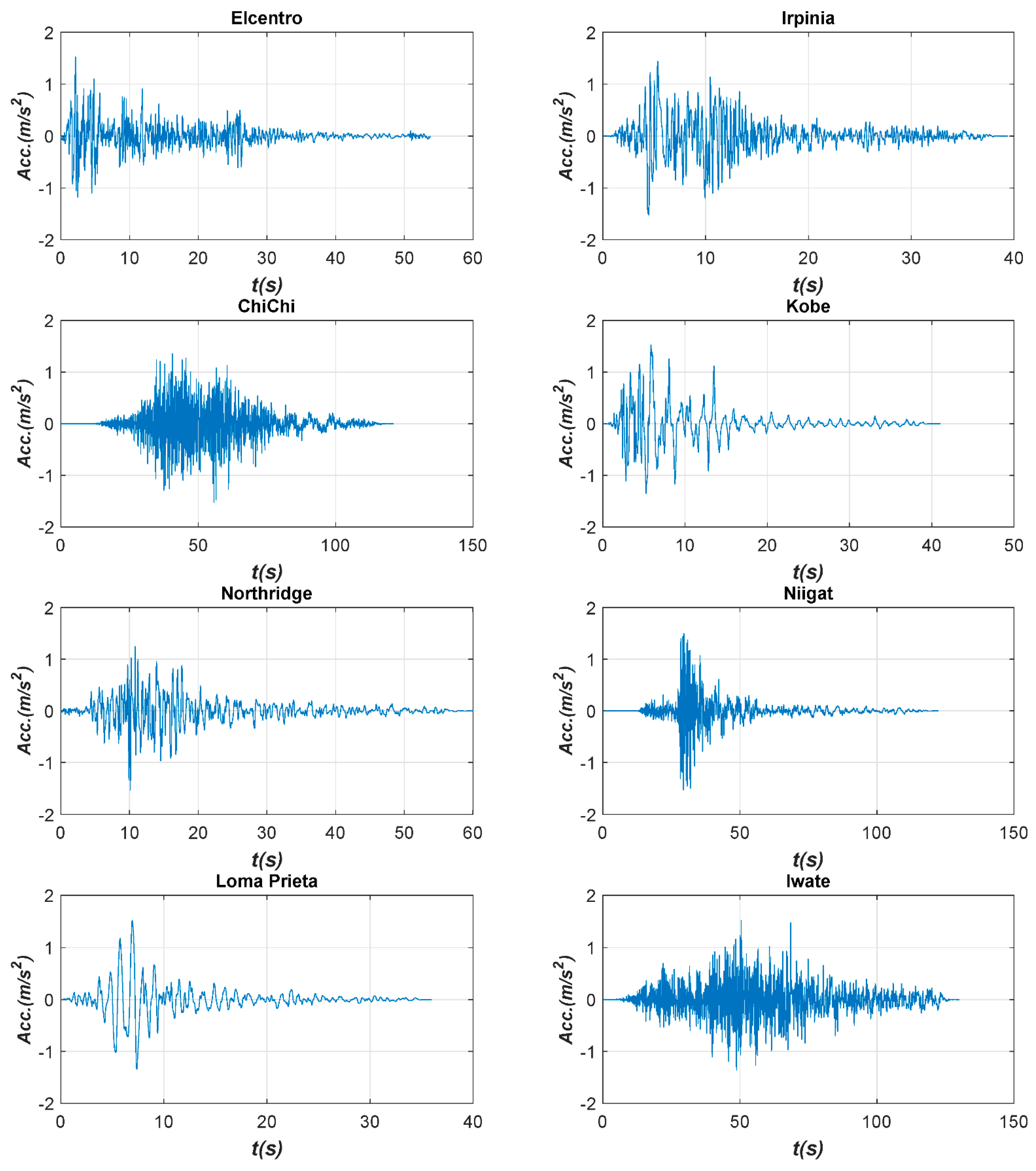
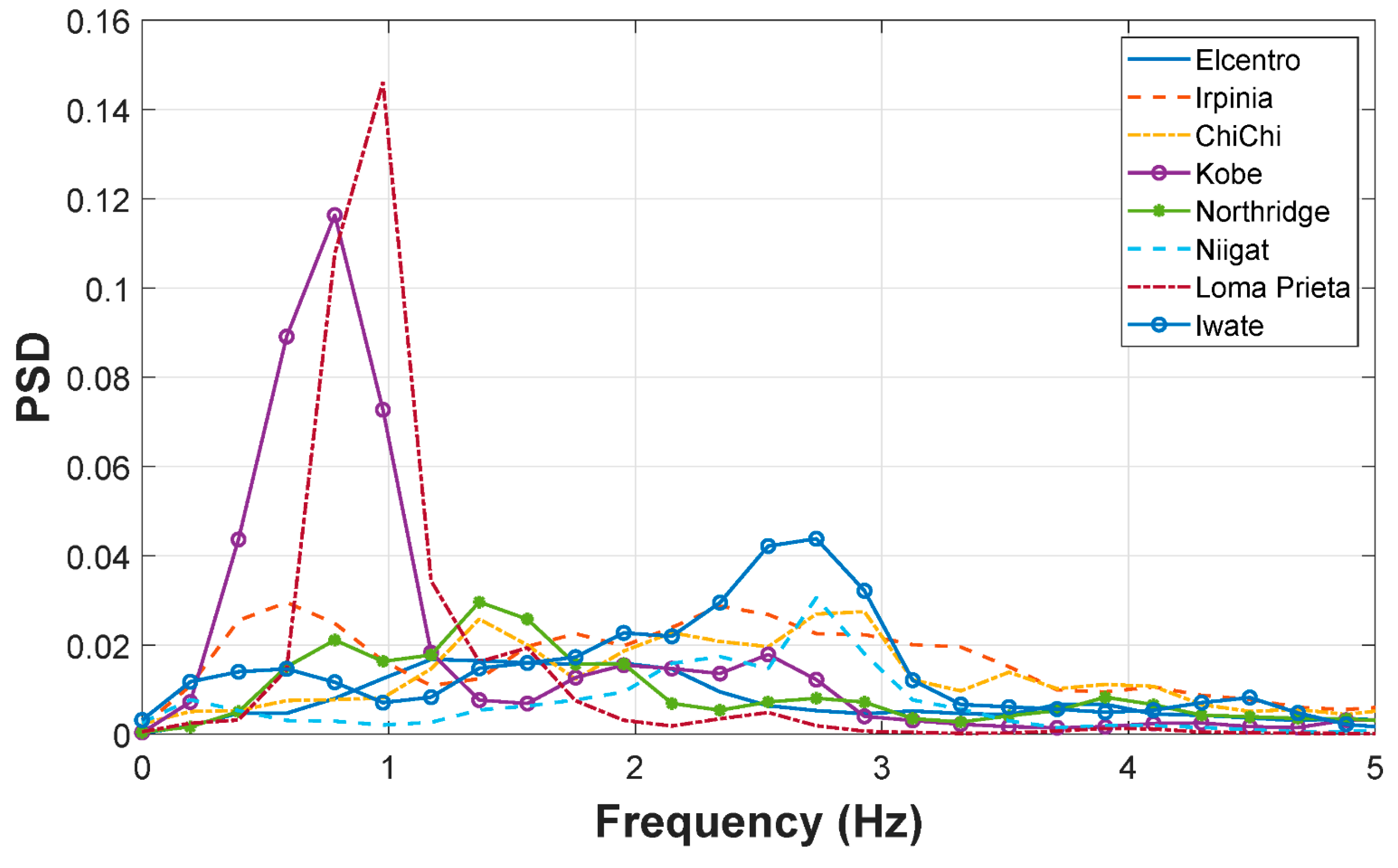
4.3.1. Characteristics of Selected Ground Motions

In this study, eight sets of ground motions are selected for the seismic response analysis, i.e., Elcentro wave, Irpinia wave, Chichi wave, Kobe wave, Northridge wave, Niigat wave, Loma Prieta wave and Iwate wave. Their time histories are shown in Figure 7 and their power spectral densities (PSDs) are shown in Figure 8. All of these ground motions are processed with amplitude modulations such that the peak ground accelerations (PGAs) are set to be 1.5247 m/s². From Figure 8, it can be seen that Kobe and Loma Prieta are long period ground motions in which low frequency components have taken up a large scale in the whole frequency domain, and the others are standard seismic waves which contain plenty of high-frequency components.

4.3.2. Displacement and Acceleration Responses to Real Earthquakes

The system parameters are the same as before, and the responses to different ground motions are calculated using the Runge-Kutta algorithm. The peak displacement responses (PDRs) and the peak acceleration responses (PARs) are shown in

Table 1. Peak displacement responses (PDRs) of SDOF-ECDs and SDOF-FVDs.

Seismic Wave	Without Damper (m)	FVD-SDOF			ECD-SDOF
		$\mathit{\alpha }$	PDR (m)	$\mathit{\rho }$	PDR (m)	$\mathit{\rho }$
Elcentro	0.1553	0.2	0.0097	93.75%	0.0158	89.81%
		0.4	0.0200	87.12%	0.0186	88.04%
		0.6	0.0324	79.12%	0.0273	82.43%
		0.8	0.0404	73.96%	0.0333	78.56%
		1	0.0498	67.91%	0.0441	71.63%
Irpinia	0.1977	0.2	0.0399	79.82%	0.0416	78.97%
		0.4	0.0634	67.92%	0.0579	70.69%
		0.6	0.0846	57.22%	0.0724	63.39%
		0.8	0.1033	47.75%	0.0890	54.95%
		1	0.1155	41.54%	0.1049	46.94%
ChiChi	1.0532	0.2	0.0225	97.86%	0.0225	97.86%
		0.4	0.0321	96.95%	0.0316	97.00%
		0.6	0.0460	95.63%	0.0417	96.04%
		0.8	0.0967	90.81%	0.0561	94.67%
		1	0.1640	84.43%	0.0787	92.53%
Kobe	0.1271	0.2	0.0817	35.67%	0.0778	38.80%
		0.4	0.0883	30.48%	0.0802	36.89%
		0.6	0.0950	25.24%	0.0863	32.11%
		0.8	0.0963	24.19%	0.0936	26.37%
		1	0.0969	23.76%	0.0981	22.80%
Northridge	0.1441	0.2	0.0178	87.68%	0.0161	88.82%
		0.4	0.0300	79.18%	0.0248	82.76%
		0.6	0.0373	74.13%	0.0329	77.15%
		0.8	0.0458	68.23%	0.0396	72.50%
		1	0.0578	59.92%	0.0447	68.97%
Niigat	0.4533	0.2	0.0220	95.14%	0.0252	94.43%
		0.4	0.0426	90.59%	0.0384	91.52%
		0.6	0.0721	84.10%	0.0554	87.77%
		0.8	0.1208	73.34%	0.0795	82.47%
		1	0.1733	61.77%	0.1023	77.44%
Loma Prieta	0.1475	0.2	0.0749	49.21%	0.0636	56.84%
		0.4	0.0652	55.80%	0.0669	54.62%
		0.6	0.0646	56.17%	0.0687	53.43%
		0.8	0.0636	56.86%	0.0695	52.89%
		1	0.0684	53.59%	0.0673	54.34%
Iwate	0.6960	0.2	0.0466	93.30%	0.0362	94.81%
		0.4	0.0629	90.96%	0.0511	92.66%
		0.6	0.0830	88.07%	0.0726	89.57%
		0.8	0.1304	81.26%	0.0931	86.62%
		1	0.1767	74.61%	0.1150	83.48%

and

Table 2. Peak acceleration responses (PARs) of SDOF-ECDs and SDOF-FVDs.

Seismic Wave	Without Damper (m/s2)	SDOF-FVD			SDOF-ECD
		$\mathit{\alpha }$	PAR (m/s2)	$\mathit{\rho }$	PAR (m/s2)	$\mathit{\rho }$
Elcentro	2.98	0.2	2.57	13.60%	2.55	14.43%
		0.4	2.69	9.58%	2.59	13.09%
		0.6	2.72	8.68%	2.75	7.54%
		0.8	2.88	3.13%	2.81	5.54%
		1	2.93	1.59%	2.86	3.99%
Irpinia	3.08	0.2	2.96	3.92%	3.05	0.89%
		0.4	2.84	7.80%	2.84	7.77%
		0.6	2.98	3.29%	2.92	5.16%
		0.8	2.98	3.12%	2.94	4.40%
		1	3.01	2.20%	2.97	3.39%
ChiChi	3.26	0.2	2.57	21.14%	2.56	21.54%
		0.4	2.78	14.67%	2.74	15.78%
		0.6	2.91	10.83%	2.85	12.70%
		0.8	2.97	8.72%	2.92	10.51%
		1	3.05	6.49%	2.95	9.47%
Kobe	3.13	0.2	2.54	18.77%	2.54	18.71%
		0.4	2.81	10.21%	2.78	11.26%
		0.6	3.02	3.48%	2.92	6.75%
		0.8	3.11	0.71%	3.02	3.45%
		1	3.12	0.42%	3.08	1.70%
Northridge	2.99	0.2	2.55	14.65%	2.51	15.96%
		0.4	2.71	9.43%	2.66	11.00%
		0.6	2.85	4.72%	2.75	7.91%
		0.8	2.92	2.14%	2.87	4.07%
		1	2.98	0.26%	2.90	2.88%
Niigat	3.10	0.2	2.79	10.10%	2.78	10.52%
		0.4	2.94	5.22%	2.88	6.99%
		0.6	2.96	4.48%	2.94	5.16%
		0.8	3.01	3.03%	2.97	4.17%
		1	3.01	2.85%	2.99	3.45%
Loma Prieta	3.11	0.2	3.14	−1.16%	2.96	4.63%
		0.4	3.06	1.49%	3.03	2.35%
		0.6	2.97	4.51%	3.03	2.46%
		0.8	2.96	4.77%	2.97	4.34%
		1	3.02	2.80%	2.94	5.34%
Iwate	3.18	0.2	2.61	17.77%	2.82	11.19%
		0.4	2.98	6.15%	2.96	6.75%
		0.6	3.03	4.49%	3.03	4.62%
		0.8	3.12	1.88%	3.07	3.47%
		1	3.09	2.73%	3.09	2.58%

, respectively. Here, we define the response reduction ratio ρ as follows

$$\rho =\frac{A_o - A_d}{A_o}$$

(9)

where A_o is the peak displacement or acceleration response without a damper and A_d is the peak displacement or acceleration response with a damper. The larger the reduction ratio, the better the response control performance of supplemental devices. The reduction ratios of displacement and acceleration are compared for ECDs and FVDs in Figure 9 and Figure 10, respectively. The points above the zero line indicate that the control performance of ECD is better than that of FVD, and vice versa. From Figure 9 and Figure 10, it is found that the displacement and acceleration reduction ratios of ECDs are larger than those of FVDs in most cases, and the displacement reduction ratios are generally greater than the acceleration reduction ratios for both ECDs and FVDs. It should also be pointed out that there are still some cases where ECDs do not work better than FVDs for Kobe and Loma Prieta seismic waves. In the previous Section 4.2, it is found that although the control performance of the ECDs are better than that of FVDs in the resonance frequency band, in the frequency band of a certain distance from the resonance or far from the resonance, the control performance of the ECDs are slightly worse in some cases. That is the reason why ECDs do not work better than FVDs when the dominant frequency band of the seismic excitation is far from the resonance.

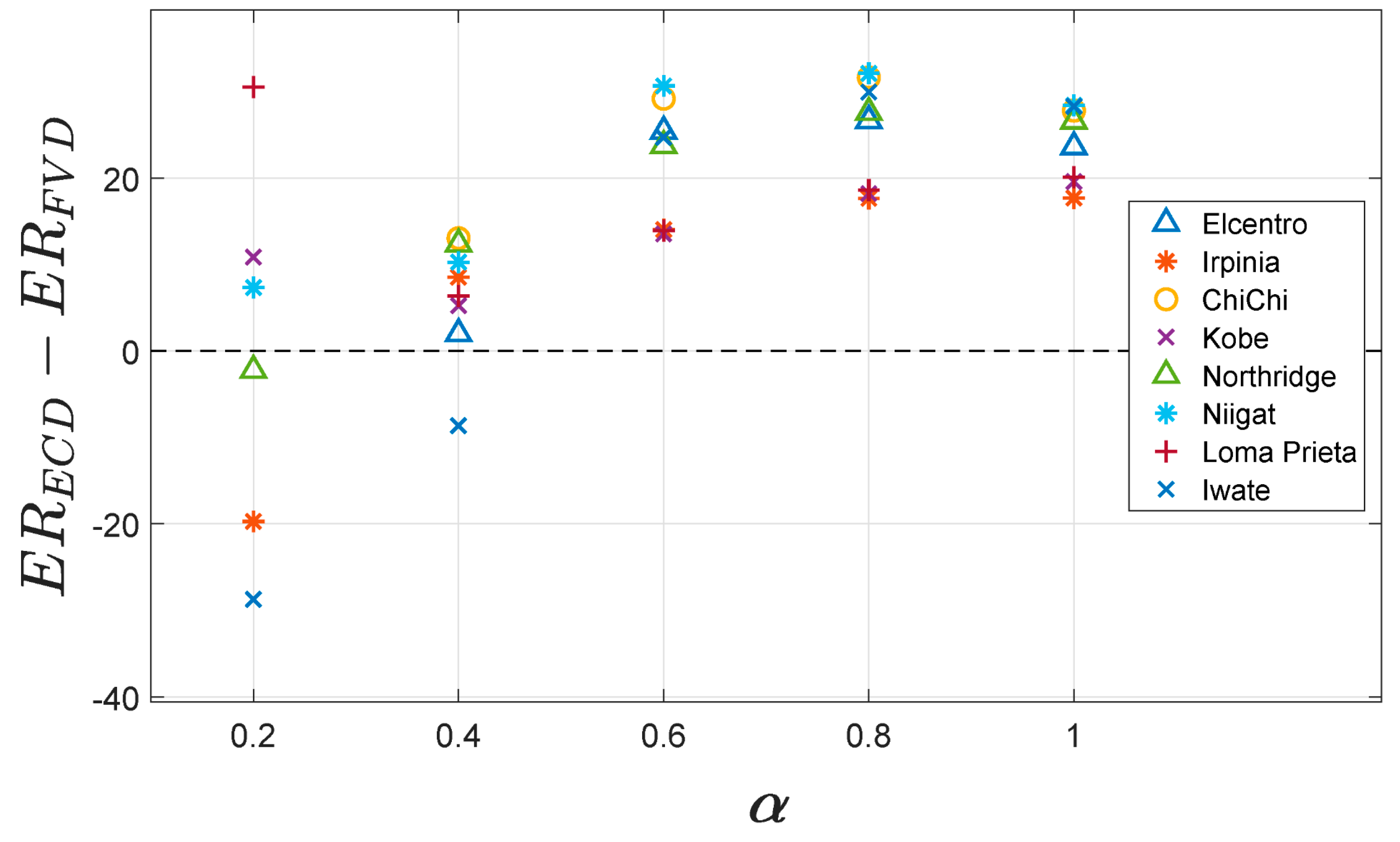
4.3.3. Energy Dissipation Analysis Under Seismic Excitations

For elastic SDOF systems, the input energy of seismic excitations will be finally dissipated by the structural inherent damping and supplemental damping devices. In this paper, the energy dissipated by the inherent damping is expressed as

$$E_{in}={{\displaystyle \int }}_0^{T_t}c\dot{u}\dot{u}dt={{\displaystyle \int }}_0^{T_t}2\zeta m{\omega }_n\dot{u}\dot{u}dt$$

(10)

where T_t is the duration of the ground motions. The energy dissipated by the supplemental damping devices (ECDs or FVDs) is

$$E_{ECD(FVD)}={{\displaystyle \int }}_0^{T_t}{F}_{ECD(FVD)}(\dot{u})\dot{u}dt$$

(11)

The total dissipated energy is

$$E_{total}=E_{in}+E_{ECD(FVD)}$$

(12)

The time history results of the normalized dissipated energy of FVD and ECD subjected to the Elcentro ground motion are shown in Figure 11. As shown in Figure 11a, the normalized energy dissipated by the FVD (α = 1) is 0.9648, which is 27.38 times of that dissipated by the corresponding inherent damping (0.0352), indicating that the FVD improves the energy dissipation capability of uncontrolled systems by 27.38 times. As a contrast, it is clear that in Figure 11b, the energy dissipated by the ECD is larger than the energy dissipated by the FVD. Specifically, the normalized energy dissipated by the ECD in Figure 11b is 0.9808, which is about 50.98 times of the energy dissipated by the corresponding inherent damping (0.0192). These results indicate that the ECD could improve the energy dissipation capability of uncontrolled systems by about 50.98 times.

As indicated by Equation (10), if the inherent damping is prescribed, the energy dissipated by the inherent damping depends on the response amplitude. To protect the structure, the supplemental damping devices are required to dissipate the majority of the input seismic energy. Here, we define a new criterion named as the energy dissipation ratio (ER) to represent the energy dissipation capacity of supplemental damping devices. The larger the energy dissipative ratio, the larger the energy dissipation capability of supplemental devices.

$${\mathrm{ER}}_{ECD(FVD)}=\frac{{\mathrm{E}}_{ECD(FVD)}}{{\mathrm{E}}_{in}}$$

(13)

The energy dissipation ratios of the SDOF systems (ζ = 2%) with FVDs and ECDs subjected to different ground motions are compared in

Table 3. Energy dissipation ratios (ERs) of SDOF-ECDs and SDOF-FVDs.

Seismic Wave	SDOF-FVD			SDOF-ECD
	$\mathit{\alpha }$	Normalized Energy	ER		Normalized Energy	ER
Elcentro	0.2	0.9974	383.51		0.9967	302.27
	0.4	0.9946	183.40		0.9946	185.37
	0.6	0.9892	91.83		0.9915	117.22
	0.8	0.9801	49.14		0.9870	75.77
	1	0.9648	27.38		0.9808	50.98
Irpinia	0.2	0.9955	219.02		0.9950	199.28
	0.4	0.9914	114.72		0.9920	123.24
	0.6	0.9857	68.99		0.9881	83.02
	0.8	0.9771	42.62		0.9837	60.25
	1	0.9649	27.50		0.9783	45.18
ChiChi	0.2	0.9976	424.25		0.9973	372.16
	0.4	0.9947	187.15		0.9950	200.18
	0.6	0.9894	92.95		0.9919	122.12
	0.8	0.9798	48.40		0.9877	80.03
	1	0.9649	27.50		0.9822	55.29
Kobe	0.2	0.9919	122.42		0.9926	133.27
	0.4	0.9892	91.89		0.9898	97.12
	0.6	0.9839	60.99		0.9868	74.52
	0.8	0.9759	40.58		0.9833	58.78
	1	0.9649	27.50		0.9792	47.06
Northridge	0.2	0.9974	383.35		0.9974	381.09
	0.4	0.9943	173.06		0.9946	185.42
	0.6	0.9889	89.46		0.9912	113.20
	0.8	0.9799	48.71		0.9871	76.30
	1	0.9649	27.50		0.9818	54.08
Niigat	0.2	0.9968	315.39		0.9969	322.72
	0.4	0.9944	178.90		0.9947	189.16
	0.6	0.9889	89.25		0.9917	119.90
	0.8	0.9789	46.43		0.9874	78.53
	1	0.9649	27.50		0.9824	55.89
Loma Prieta	0.2	0.9910	110.46		0.9930	140.99
	0.4	0.9895	94.66		0.9902	101.01
	0.6	0.9843	62.67		0.9871	76.57
	0.8	0.9763	41.12		0.9835	59.72
	1	0.9649	27.47		0.9794	47.57
Iwate	0.2	0.9966	296.45		0.9963	267.73
	0.4	0.9942	171.17		0.9939	162.51
	0.6	0.9882	83.77		0.9909	108.47
	0.8	0.9785	45.54		0.9869	75.48
	1	0.9649	27.50		0.9824	55.78

and Figure 12. From Figure 12, the points above the zero line indicate that the energy dissipation capacity of ECD is better than that of FVD, and vice versa. It is found that the energy dissipation capacity of ECDs are larger than those of FVDs in most cases.

5. Conclusions

This paper investigates the dynamic characteristics of a rotary axial ECD and its seismic reduction performance when applied in a linear elastic SDOF system. The nonlinear force-velocity relationship of the ECD is expressed using the Wouterse’s model which are validated by Finite element simulation and experimental testing. The energy dissipation capacity of the ECD is obtained analytically and its optimal parameters for maximum energy dissipation are also derived. The control performance of ECDs is investigated and evaluated under harmonic excitations and real earthquake ground motions. The most important findings are summarized below:

(1)

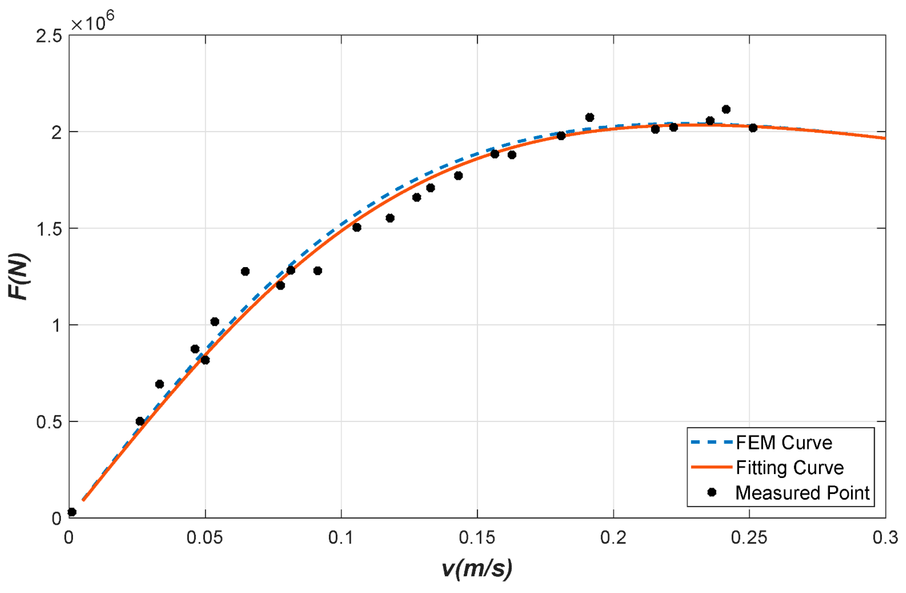
The force-velocity constitutive behavior of the ECD can be well depicted by the Wouterse’s model. The eddy current damping force is linearly proportional to the velocity for low speed region, gradually increasing with decreasing slope when the velocity become higher, reaching a maximum at the critical speed, and then decreasing for much higher speeds. These unique characteristics can protect the damper and structure from damage when an over-load is exerted on the damper.

(2)

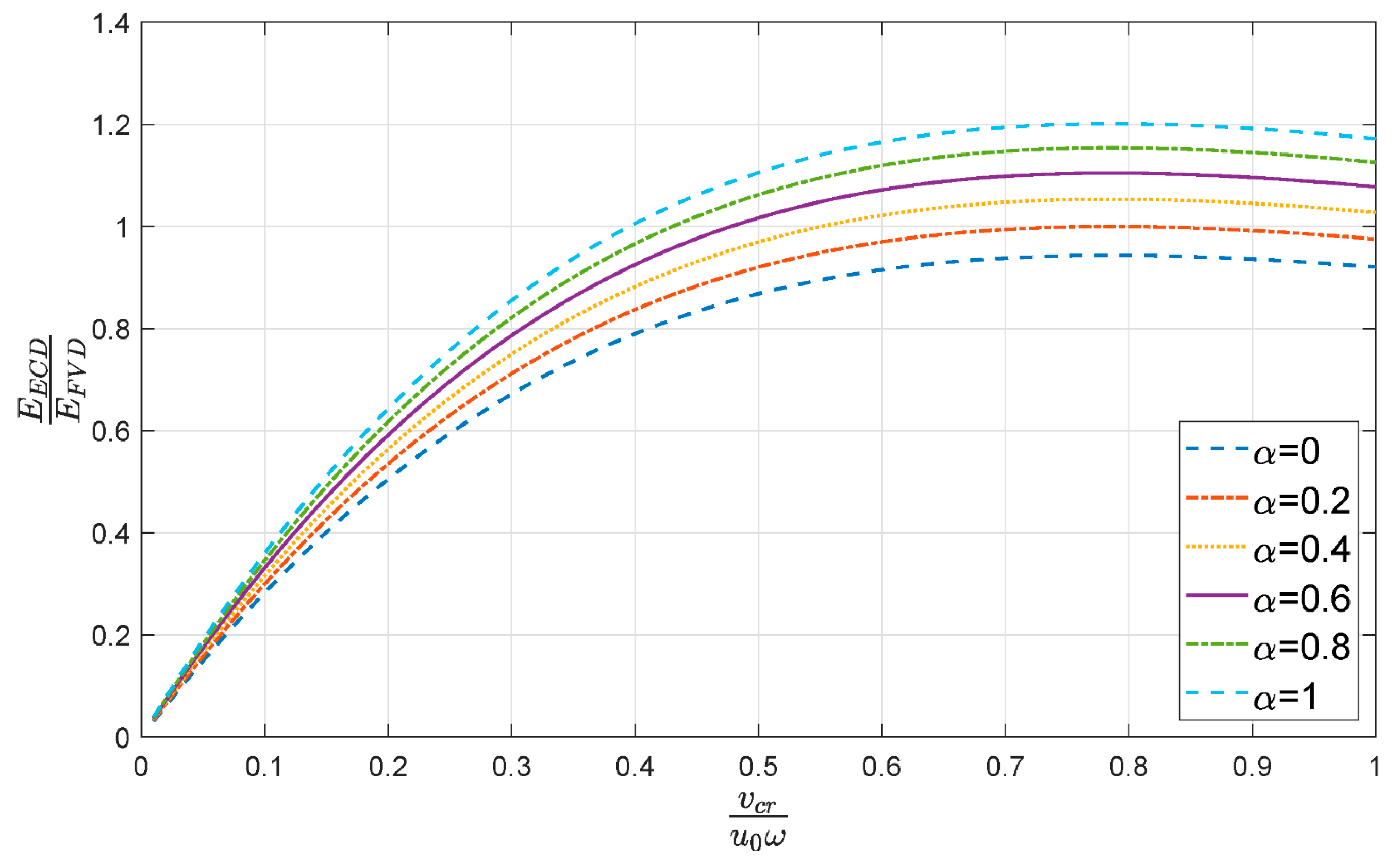
When the ratio of the critical velocity of the ECD to the maximum velocity is 0.786, the energy dissipation capacity of ECD reaches its maximum under harmonic motions. It always can find a better design of ECD when the velocity exponent α of FVD is larger than 0.2 such that the energy dissipation capacity of ECD is larger than that of FVD under the same harmonic motion.

(3)

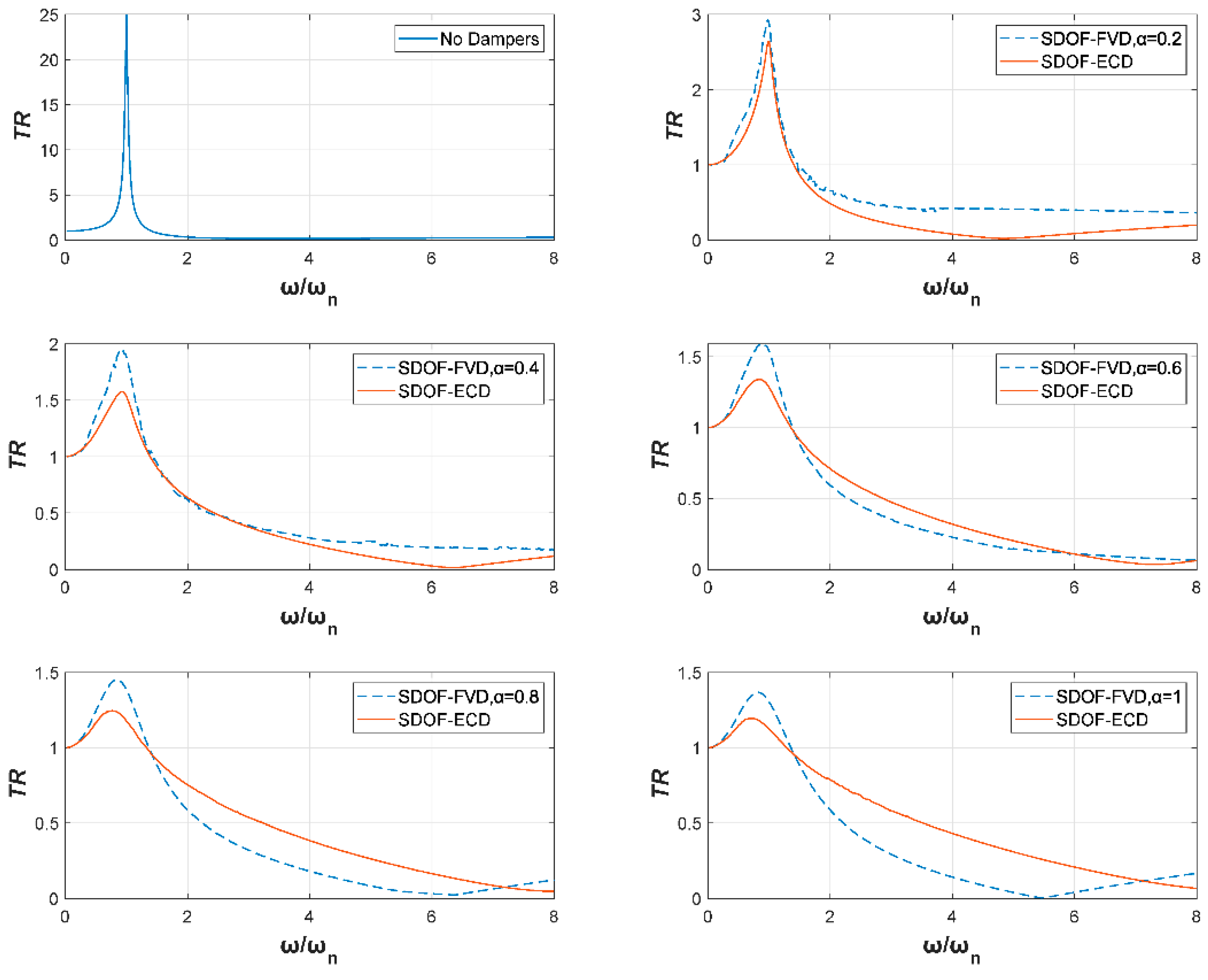
In the resonance frequency band, both the displacement and acceleration responses of SDOF-ECDs are smaller than those of SDOF-FVDs under the same harmonic excitation. As the velocity exponent α of the FVD increases, the control performance of the corresponding ECD gets better and better compared with that of FVD.

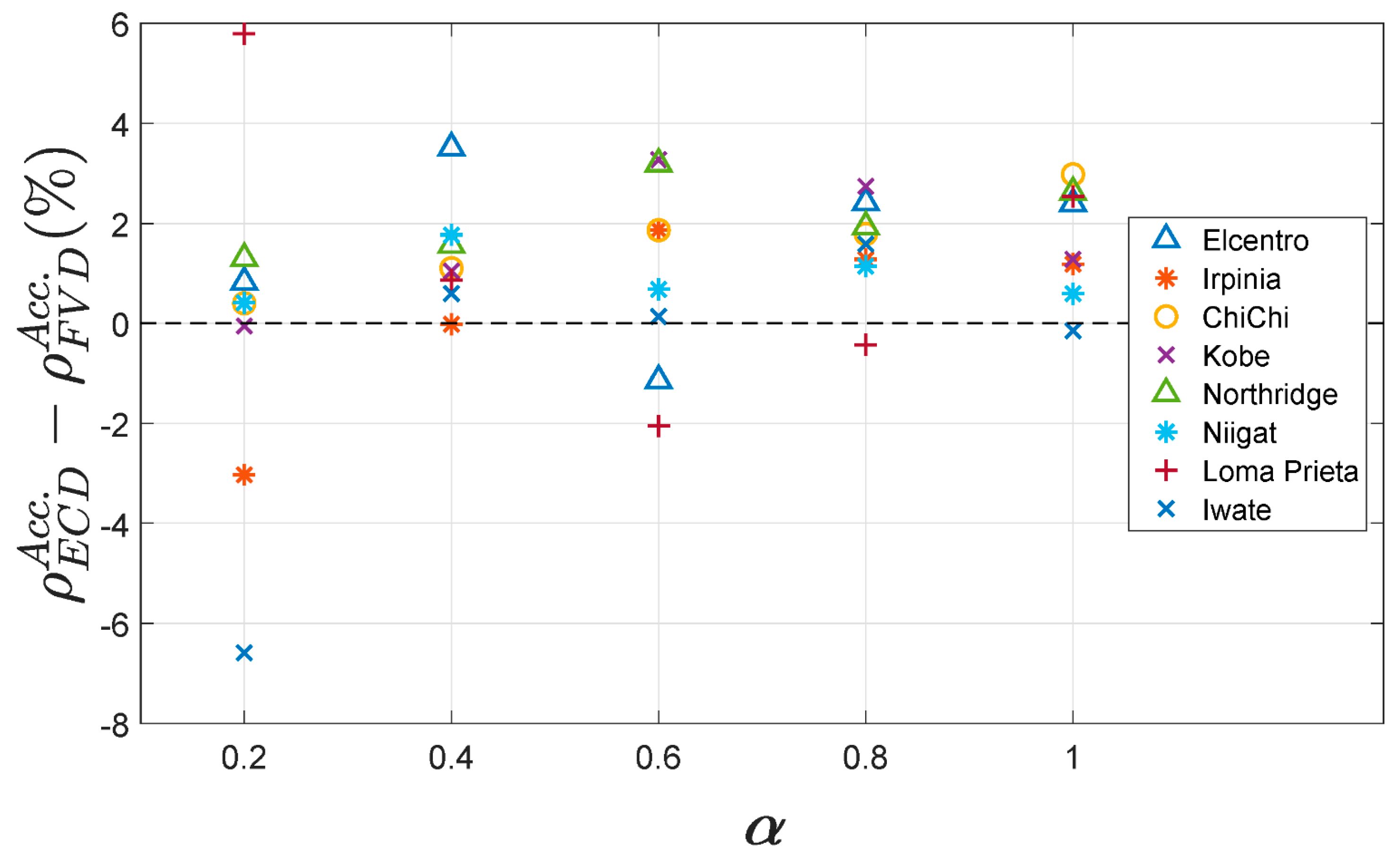
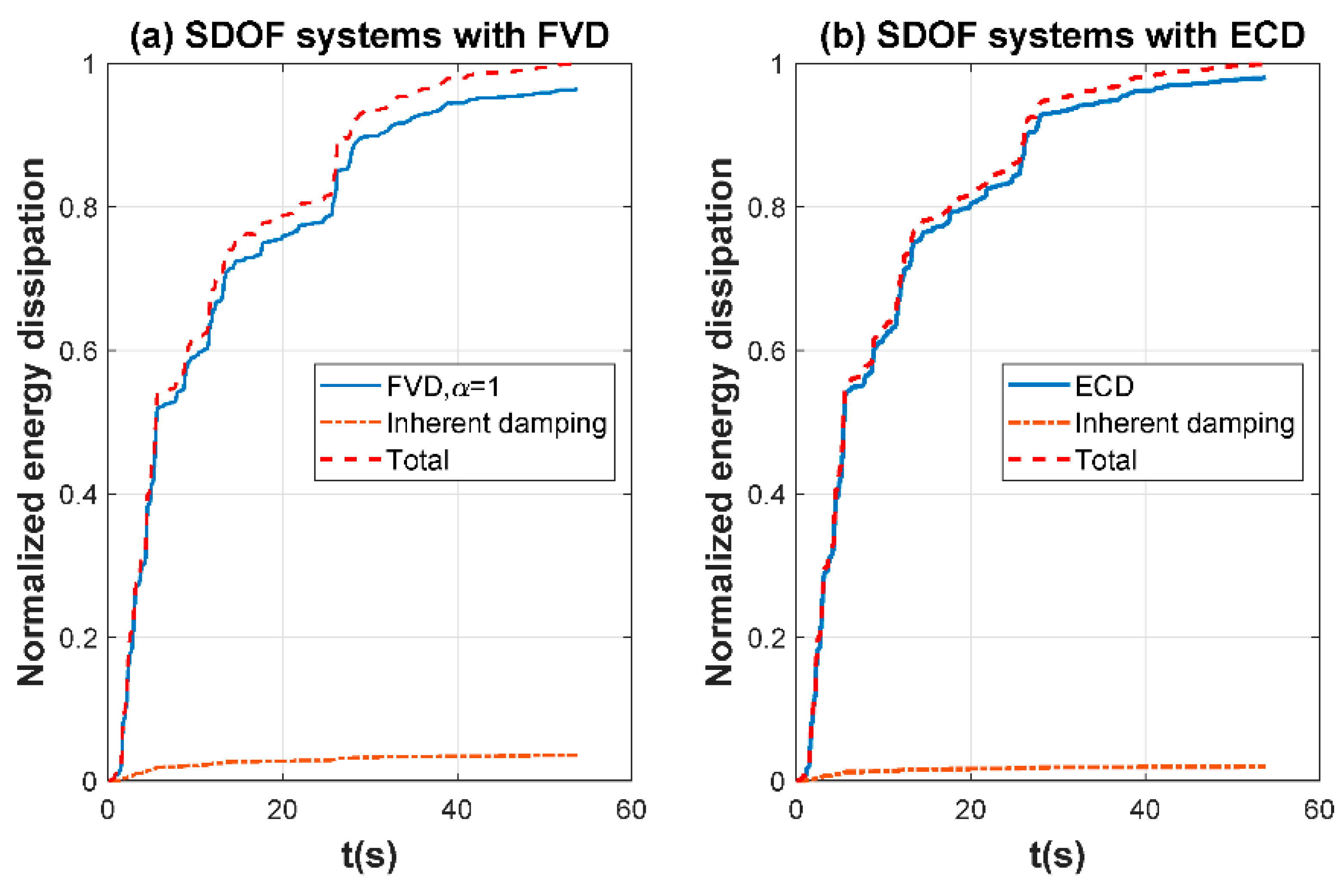
(4)

The displacement and acceleration reduction ratios of ECDs are larger than those of FVDs in most of the cases under real earthquake excitations, and the displacement reduction ratios are generally greater than the acceleration reduction ratios for both ECDs and FVDs. The energy dissipation capacity of ECDs outperforms that of FVDs in most of the cases under real earthquake excitations.

Currently, this paper is limited to the numerical evaluation of ECDs for elastic SDOF systems. The conclusions summarized above are based on the limited data presented in this paper. To further extrapolate the findings, the next step is to experimentally test the performance of ECDs with structures. Meanwhile, the further studies on applying ECDs in MDOF systems will also be developed in the future.

References

1. Lu, X.; Chen, J. Mitigation of wind-induced response of Shanghai Center Tower by tuned mass damper. Struct. Des. Tall Spec. Build. 2011, 20, 435–452. [Google Scholar] [CrossRef]
2. Lu, X.; Zhang, Q.; Weng, D.; Zhou, Z.; Wang, S.; Mahin, S.A.; Ding, S.; Qian, F. Improving performance of a super tall building using a new eddy-current tuned mass damper. Struct. Control Health Monit. 2017, 24, e1882. [Google Scholar] [CrossRef]
3. Ji, X.; Liu, D.; Hutt, C.M. Seismic performance evaluation of a high-rise building with novel hybrid coupled walls. Eng. Struct. 2018, 169, 216–225. [Google Scholar] [CrossRef]
4. Qian, H.; Li, H.; Song, G. Experimental investigations of building structure with a superelastic shape memory alloy friction damper subject to seismic loads. Smart Mater. Struct. 2016, 25, 125056. [Google Scholar] [CrossRef]
5. Li, L.; Song, G.; Ou, J. Hybrid active mass damper (AMD) vibration suppression of nonlinear high-rise structure using fuzzy logic control algorithm under earthquake excitations. Struct. Control Health Monit. 2011, 18, 698–709. [Google Scholar] [CrossRef]
6. Guo, T.; Liu, J.; Zhang, Y.; Pan, S. Displacement Monitoring and Analysis of Expansion Joints of Long-Span Steel Bridges with Viscous Dampers. J. Bridge Eng. 2015, 20, 04014099. [Google Scholar] [CrossRef]
7. Yang, M.-G.; Chen, Z.-Q.; Hua, X.-G. An experimental study on using MR damper to mitigate longitudinal seismic response of a suspension bridge. Soil Dyn. Earthq. Eng. 2011, 31, 1171–1181. [Google Scholar] [CrossRef]
8. Li, C.; Li, H.-N.; Hao, H.; Bi, K.; Chen, B. Seismic fragility analyses of sea-crossing cable-stayed bridges subjected to multi-support ground motions on offshore sites. Eng. Struct. 2018, 165, 441–456. [Google Scholar] [CrossRef]
9. Wen, Q.; Hua, X.G.; Chen, Z.Q.; Yang, Y.; Niu, H.W. Control of Human-Induced Vibrations of a Curved Cable-Stayed Bridge: Design, Implementation, and Field Validation. J. Bridge Eng. 2016, 21, 04016028. [Google Scholar] [CrossRef]
10. Varela, W.D.; Battista, R.C. Control of vibrations induced by people walking on large span composite floor decks. Eng. Struct. 2011, 33, 2485–2494. [Google Scholar] [CrossRef]
11. Li, H.; Liu, M.; Li, J.; Guan, X.; Ou, J. Vibration Control of Stay Cables of the Shandong Binzhou Yellow River Highway Bridge Using Magnetorheological Fluid Dampers. J. Bridge Eng. 2007, 12, 401–409. [Google Scholar] [CrossRef]
12. Chen, Z.Q.; Wang, X.Y.; Ko, J.M.; Ni, Y.Q.; Spencer, B.F.; Yang, G.; Hu, J.H. MR damping system for mitigating wind-rain induced vibration on Dongting Lake Cable-Stayed Bridge. Wind Struct. 2004, 7, 293–304. [Google Scholar] [CrossRef]
13. Shi, X.; Zhu, S.; Li, J.-Y.; Spencer, B.F., Jr. Dynamic behavior of stay cables with passive negative stiffness dampers. Smart Mater. Struct. 2016, 25, 075044. [Google Scholar] [CrossRef]
14. Zhang, Z.; Staino, A.; Basu, B.; Nielsen, S.R.K. Performance evaluation of full-scale tuned liquid dampers (TLDs) for vibration control of large wind turbines using real-time hybrid testing. Eng. Struct. 2016, 126, 417–431. [Google Scholar] [CrossRef]
15. Zhang, Z.; Nielsen, S.R.K.; Basu, B.; Li, J. Nonlinear modeling of tuned liquid dampers (TLDs) in rotating wind turbine blades for damping edgewise vibrations. J. Fluids Struct. 2015, 59, 252–269. [Google Scholar] [CrossRef]
16. Zuo, H.; Bi, K.; Hao, H. Using multiple tuned mass dampers to control offshore wind turbine vibrations under multiple hazards. Eng. Struct. 2017, 141, 303–315. [Google Scholar] [CrossRef]
17. Song, G.B.; Zhang, P.; Li, L.Y.; Singla, M.; Patil, D.; Li, H.N.; Mo, Y.L. Vibration Control of a Pipeline Structure Using Pounding Tuned Mass Damper. J. Eng. Mech. 2016, 142, 04016031. [Google Scholar] [CrossRef]
18. Lin, W.-H.; Chopra, A.K. Earthquake response of elastic SDF systems with non-linear fluid viscous dampers. Earthq. Eng. Struct. Dyn. 2002, 31, 1623–1642. [Google Scholar] [CrossRef]
19. Wang, W.; Wang, X.; Hua, X.; Song, G.; Chen, Z. Vibration control of vortex-induced vibrations of a bridge deck by a single-side pounding tuned mass damper. Eng. Struct. 2018, 173, 61–75. [Google Scholar] [CrossRef]
20. Lin, W.; Song, G.; Chen, S. PTMD Control on a Benchmark TV Tower under Earthquake and Wind Load Excitations. Appl. Sci. 2017, 7, 425. [Google Scholar] [CrossRef]
21. Zhang, P.; Song, G.; Li, H.-N.; Lin, Y.-X. Seismic Control of Power Transmission Tower Using Pounding TMD. J. Eng. Mech. 2013, 139, 1395–1406. [Google Scholar] [CrossRef]
22. Huang, Z.W.; Hua, X.G.; Chen, Z.Q.; Niu, H.W. Modeling, Testing, and Validation of an Eddy Current Damper for Structural Vibration Control. J. Aerosp. Eng. 2018, 31, 04018063. [Google Scholar] [CrossRef]
23. Shen, W.; Zhu, S.; Xu, Y. An experimental study on self-powered vibration control and monitoring system using electromagnetic TMD and wireless sensors. Sens. Actuators A Phys. 2012, 180, 166–176. [Google Scholar] [CrossRef] [Green Version]
24. Shen, W.; Zhu, S.; Zhu, H.; Xu, Y. Electromagnetic energy harvesting from structural vibrations during earthquakes. Smart Struct. Syst. 2016, 18, 449–470. [Google Scholar] [CrossRef]
25. Shen, W.; Zhu, S.; Zhu, H. Unify Energy Harvesting and Vibration Control Functions in Randomly Excited Structures with Electromagnetic Devices. J. Eng. Mech. 2019, 145, 04018115. [Google Scholar] [CrossRef]
26. Zuo, L.; Chen, X.; Nayfeh, S. Design and Analysis of a New Type of Electromagnetic Damper With Increased Energy Density. J. Vib. Acoust. 2011, 133, 041006. [Google Scholar] [CrossRef]
27. Chen, Z. Outer Cup Rotary Axial Eddy Current Damper. 15 September 2014. [Google Scholar]
28. Pérez-Díaz, J.; Valiente-Blanco, I.; Cristache, C. Z-Damper: A New Paradigm for Attenuation of Vibrations. Machines 2016, 4, 12. [Google Scholar] [CrossRef]
29. Wouterse, J.H. Critical torque and speed of eddy current brake with widely separated soft iron poles. IEE Proc. B (Electr. Power Appl.) 1991, 138, 153. [Google Scholar] [CrossRef]
30. Constantinou, M.C.; Soong, T.T.; Dargush, G.F. Passive Energy Dissipation Systems for Structural Design and Retrofit; MCEER Monograph No. MCEER-98-MN01, SUNY; UBIR: Buffalo, NY, USA, 1998. [Google Scholar]
31. Nehl, T.W.; Lequesne, B.; Gangla, V.; Gutkowski, S.A.; Robinson, M.J.; Sebastian, T. Nonlinear two-dimensional finite element modeling of permanent magnet eddy current couplings and brakes. IEEE Trans. Magn. 1994, 30, 3000–3003. [Google Scholar] [CrossRef]
32. Canova, A.; Vusini, B. Analytical modeling of rotating eddy-current couplers. IEEE Trans. Magn. 2005, 41, 24–35. [Google Scholar] [CrossRef]
33. Sharif, S.; Faiz, J.; Sharif, K. Performance analysis of a cylindrical eddy current brake. IET Electr. Power Appl. 2012, 6, 661. [Google Scholar] [CrossRef]
Figure 1. Cross sections of the rotary axial eddy current damper (ECD): (a) Longitudinal view; (b) transverse view.
Applsci 09 03427 g001
Figure 2. Comparison of fitting curve with measured points and FEM curve for ECDs.
Applsci 09 03427 g002
Figure 3. The energy dissipation ratio versus the velocity ratio.
Applsci 09 03427 g003
Figure 4. The schematic model of the SDOF system with a supplemental damper subjected to ground motion.
Applsci 09 03427 g004
Figure 5. Comparison of displacement response factors for SDOF-ECDs and SDOF-FVDs.
Applsci 09 03427 g005
Figure 6. Comparison of acceleration transmissibilities for SDOF-ECDs and SDOF-FVDs.
Applsci 09 03427 g006
Figure 7. Time histories of ground motions.
Applsci 09 03427 g007
Figure 8. Power spectral densities of ground motions.
Applsci 09 03427 g008
Figure 9. Displacement reduction ratios under different earthquakes.
Applsci 09 03427 g009
Figure 10. Acceleration reduction ratios under different earthquakes.
Applsci 09 03427 g010
Figure 11. Dissipated energy of SDOF systems (ζ = 2%) with FVD and ECD subjected to the Elcentro earthquake.
Applsci 09 03427 g011
Figure 12. Energy dissipation ratios under different earthquakes.
Applsci 09 03427 g012