Article

Research on Collaborative Optimization of Green Manufacturing in Semiconductor Wafer Distributed Heterogeneous Factory

1
Business School, University of Shanghai for Science & Technology, Shanghai 200093, China
2
Henan Institute of Technology, Xinxiang 453000, China
*
Author to whom correspondence should be addressed.
Appl. Sci. 2019, 9(14), 2879; https://doi.org/10.3390/app9142879
Submission received: 6 June 2019 / Revised: 12 July 2019 / Accepted: 15 July 2019 / Published: 18 July 2019

Abstract

:
Production scheduling of semiconductor wafer manufacturing is a challenging research topic in the field of industrial engineering. Based on this, the green manufacturing collaborative optimization problem of the semiconductor wafer distributed heterogeneous factory is first proposed, which is also a typical NP-hard problem with practical application value and significance. To solve this problem, it is very important to find an effective algorithm for rational allocation of jobs among various factories and the production scheduling of allocated jobs within each factory, so as to realize the collaborative optimization of the manufacturing process. In this paper, a scheduling model for green manufacturing collaborative optimization of the semiconductor wafer distributed heterogeneous factory is constructed. By designing a new learning strategy of initial population and leadership level, designing a new search strategy of the predatory behavior for the grey wolf algorithm, which is a new swarm intelligence optimization algorithm proposed in recent years, the diversity of the population is expanded and the local optimum of the algorithm is avoided. In the experimental stage, two factories’ and three factories’ test cases are generated, respectively. The effectiveness and feasibility of the algorithm proposed in this paper are verified through the comparative study with the improved Grey Wolf Algorithms—MODGWO, MOGWO, the fast and elitist multi-objective genetic algorithm—NSGA-II.

1. Introduction

With the advent of the fourth industrial revolution in the context of industrial 4.0, intelligent manufacturing has become a symbol of the new information age. The semiconductor industry, as the cornerstone of the information age, belongs to the high-tech industry and faces many opportunities and challenges. While it brings high profits, fierce industry competition also forces semiconductor manufacturers to continuously improve production efficiency and resource utilization [1]. In a semiconductor manufacturing process, wafer manufacturing is called the front-end process while wafer testing and packaging is called the back-end process. Because the equipment used in wafer manufacturing are expensive and the processing process is complex, it has attracted wide attention of scholars at home and abroad. Re-entrant is a remarkable feature of semiconductor wafer fabrication [2,3,4], which means that the jobs may repeatedly access certain devices at different stages of the processing process. More than one machine with at least one stage is used for processing. In addition, during the processing of the wafer, various physical and chemical processing steps are needed to form a required circuit layer on the surface of the wafer, and the processing steps involved mainly include oxidation, deposition, implantation, sputtering, photolithography, etching, and cleaning, etc. There are strict order constraints between operations. The manufacturing process can be reduced to the reentrant hybrid flow shop (RHFS) problem, which has been proven to be an NP-hard (Non-deterministic polynomial hard) problem [5]. Because of its large scale and high complexity, the RHFS problem is difficult to solve effectively in an acceptable time using traditional mathematical modeling methods. In addition, according to the “no free lunch” theorem [6], no algorithm can achieve better results for all application problems, so it is of great significance and value to design and develop new intelligent optimization algorithms. Bertel et al. [7] proposed an integer linear programming formulation of the hybrid flow shop with recirculation, and minimizing the weighted number of tardy jobs was regarded as the optimization goal. Then a lower bound, a greedy algorithm, and a genetic algorithm were described as approximate methods. Cho et al. [8] proposed a Pareto genetic algorithm based on the Minkowski crossover operator to solve the RHFS problem, and is also designed as corresponding benchmark data sets for simulation experiments. Li et al. [9] proposed an adaptive hybrid incremental learning algorithm to solve the reentrant permutation flow shop scheduling problem with make span as the optimization objective. The degree of population evolution was evaluated by using the information entropy of the probability matrix. The mutation mechanism of the probability model and the local search method of the critical path were designed to expand the search area of the population. Huang et al. [10] designed an improved particle swarm optimization (PSO) algorithm to solve the two-stage reentrant multi-machine flow shop scheduling problem with a due window. Taking the wafer testing process as an example, aiming at minimizing the lead time or delay time, effectiveness, and robustness of the proposed algorithm were verified by large-scale test experiments. Cho et al. [11] proposed a two-level optimization algorithm to solve the reentrant flow shop problem, which satisfied the maximization of total product quantity and minimization of the customer demand delay, and applied it to real TFT-LCD (Thin Film Transistor-Liquid Crystal Display) production. To sum up, up to now, the research on the reentrant scheduling problem in domestic and foreign literature is basically based on a single production line. However, in actual production, multi-factory manufacturing and collaborative production play a key role.
Multi-factory manufacturing, including distributed manufacturing, through the cooperation of different factories distributed in different geographical locations to complete the production of products, which can rationally allocate the resources of each factory, realize the optimal combination and sharing of resources, reduce the production cost of products, and improve the satisfaction of customers, meet the diversification of customer needs. Modoni et al. [12] proposed an event-driven framework, which could realize the interaction of heterogeneous distributed resources. In particular, this research provided new mechanisms combining many technologies such as IIOT and Semantic Web, to notify significant information produced within the factory toward enabled and interested production resources. Renna et al. [13] developed a distributed approach and also used the Nash bargaining solution based on game theory, for a network of independent enterprises, which could facilitate the capacity process by using a multiagent architecture and a cooperative protocol. The simulation results demonstrated that the proposed method had a better performance when the dynamicity of the environment grows. Argoneto et al. [14] designed a framework based on a cooperative game algorithm and a fuzzy engine for capacity sharing in cloud manufacturing. The utility functions of the involved firms were taken into account in the capacity allocation policy. Xu et al. [15] proposed an effective hybrid immune algorithm to solve the distributed permutation flow shop scheduling problem by designing a new cross mutation inoculation and local search operator. Experiments showed that the algorithm was particularly effective for large-scale test problems. Zhang et al. [16] designed a distributed optimization method to solve distributed flow shop scheduling problems by reducing the power cost of manufacturing factories. Zhang et al. [17] proposed a two-stage heuristic search algorithm to solve the distributed flow shop scheduling problem with flexible assembly and installation time, with the objective of minimizing make span. Lu et al. [18] designed an improved genetic algorithm based on 3D-1D encoding and 1D-3D decoding to solve the distributed flexible job shop scheduling problem. It also introduced the allocation strategy of jobs to factories in detail. Fu et al. [19] established a stochastic multi-objective distributed permutation flow shop scheduling model considering total tardiness, make span, and total energy consumption, which also designed a new multi-objective brainstorming optimization algorithm to solve the problem. Rifai et al. [
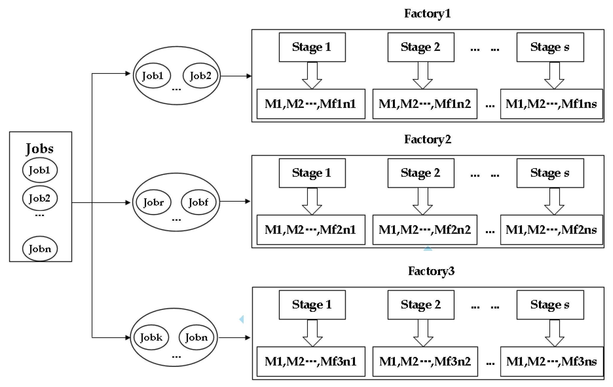
20] used the improved adaptive large neighborhood search algorithm to solve the distributed re-entrant permutation flow shop scheduling problem. It was the first time that the distributed re-entrant flow shop (DRFS) scheduling problem was studied, and it pointed out that DRFS problem was NP-Hard. To sum up, up to now, the studies on distributed scheduling problem in domestic and foreign literature is mostly confined to homogeneous factory, and most of them are research on flow shop, permutation flow shop, and flexible job shop. To the best of my knowledge, there is little research on a distributed reentrant hybrid flow shop. Distributed manufacturing of semiconductor wafers can be attributed to the distributed reentrant hybrid flow shop (DRHFS) problem, which has similar properties to the RHFS problem, but extends to multi-factory issues. Therefore, it is clear that it also belongs to the NP-Hard problem.
Environmental issues are the focus of global attention, and sustainable green manufacturing is a serious challenge for today’s manufacturing industry. Noises and CO2 emissions from the manufacturing industry are the main sources of pollution. For semiconductor wafer factories, because they are usually equipped with hundreds of precision equipment, and the wafer manufacturing process is very complex, there may be hundreds of products flowing simultaneously on the production line. Once one factory is established, it will run continuously for 365 days a year and 24 hours per day. In addition, the strict control of environmental parameters in the wafer production process makes it necessary for manufacturing factories and processing equipment to meet their production continuity requirements with uninterrupted high energy consumption. For example, precise temperature control of the etching process—the temperature fluctuation of 0.1 °C up and down will cause deviation of the wafers’ excellent rate, which results in wafer scrapping. Therefore, for semiconductor wafer manufacturing, we should not only care about the process, but also put energy saving and environmental protection on the agenda. In this paper, carbon emissions from semiconductor wafer fabrication are taken as an energy-saving indicator for research. Regarding the study of carbon emissions indicator, Zhang et al. [21] created a flexible job shop low-carbon scheduling model that considers make span, machine load, and carbon emissions indicators, and proposed a hybrid non-dominated sorting genetic algorithm II to solve the model. In order to help enterprises to quantify the carbon footprint indicator, Liu et al. [22] proposed a method for calculating the carbon footprint of workshop products and an improved fruit fly optimization algorithm to minimize the carbon footprint and production cycle of all products. Nilakantan et al. [23] developed a study on the robot assembly line system, using a multi-objective co-evolution algorithm to solve the carbon footprint minimization problem. Piroozfar et al. [24] proposed an improved multi-objective genetic algorithm to solve the multi-objective flexible job shop scheduling problem while minimizing the total carbon footprint and total number of delayed jobs. So far, there is no literature on the research of carbon emissions indicator in the semiconductor wafer manufacturing.
Grey Wolf Optimizer (GWO) is a new swarm intelligence optimization algorithm designed in 2014 by Professor Mirjalili and his team. The algorithm is inspired by the strict social hierarchy and predatory behavior of the grey wolf population in nature [25]. It is used to solve single-objective optimization problems. In 2016, Mirjalili et al. proposed a Multi-Objective Grey Wolf Optimizer (MOGWO) [26] based on the GWO algorithm to solve multi-objective optimization problems. Due to its simple algorithm structure, parameter setting, and better optimization effect, the Grey Wolf algorithm has been widely used in the research of scheduling, image processing, medical treatment, and designing photonic crystal waveguides [27,28,29,30,31]. However, there is no relevant literature about its application in green collaborative scheduling of the semiconductor wafer distributed heterogeneous factory. In summary, this paper constructs a green manufacturing collaborative optimal scheduling model for a semiconductor wafer distributed heterogeneous factory for the first time, and designs an improved multi-objective Grey Wolf Optimizer (IMOGWO) to solve this problem.
The remainder of this paper is organized as follows. The green manufacturing collaborative optimal scheduling model of the semiconductor wafer distributed heterogeneous factory is formulated in Section 2. The green collaborative scheduling problem of the semiconductor wafer distributed heterogeneous factory is described in detail in Section 3. Section 4 presents experimental results and analysis of the results. Section 5 provides the conclusions and future work.

2. Green Manufacturing Shop Scheduling Problem for Semiconductor Wafer Distributed Heterogeneous Factory

2.1. DRHFS Problem Description

Under the concept of a global cooperative sharing economy, distributed job shop scheduling has become a hot topic for scholars at home and abroad. Distributed job shop scheduling includes many dispersed factories. In addition to the characteristics of traditional job shop scheduling, collaborative optimization among factories should also be considered. n t o t a l wafers need to be assigned to F factories for processing. Because the wafer production workshop is a dust-free environment, temperature, humidity, and air quality requirements are very high. The wafer surface is protected from the oxidative corrosion of the mixed air during the processing. Therefore, wafer i can only be allocated to one factory and, once it is allocated to factory f , all operations of wafer i must be allocated to factory f for processing, which avoid discarding wafers due to contamination caused by changing the production workshop.
No replacement of the processing factory is allowed during the processing. Job scheduling and machine allocation inside the factories belong to the RHFS problem, i.e., n ( n < n t o t a l ) jobs are processed on s serial stages, and a job may need to be processed multiple times on one stage. In stage l , m l ( m l 1 ) the same parallel machines can be selected for processing. The processing time of each machine is the same, and each operation can select any machine for processing at the corresponding stage. There is no priority constraint on the processing order between jobs, but the processing order between each operation of a job has a sequential constraint. At the same time, each operation can only be processed on one machine, and each machine can only process one operation. The number of jobs’ reentrant, the number of jobs, and their processing time at each stage are fixed and known in advance. The number of production stages and the number of machines at each stage are fixed and known in advance. The capacity of buffers between successive stages is infinite. Preemption is not permitted, i.e., once an operation is started, it cannot be interrupted. The machines are continuously available for processing jobs throughout the scheduling period, and there is no maintenance, breakdown, or other interruptions. Because this paper studies the collaborative optimal scheduling problem of green manufacturing in semiconductor wafer distributed heterogeneous factory, which is assumed that all jobs can be processed in any factory, the number of production stages is the same among factories, the number of machines is different, the processing time of jobs are different in each factory, and the delivery time of jobs are different in each factory. Figure 1 is a schematic diagram of the DRHFS problem for n jobs processed in three factories.

2.2. Optimization Model of a Multi-Objective DRHFS Problem

In the multi-objective optimization problem, the objectives often conflict with each other. The enterprise decision-makers need to comprehensively consider the economic benefits as well as the social and environmental factors, and select a scheduling scheme from the Pareto solution set based on the actual production situation. In this paper, make span, total carbon emissions, and total tardiness are taken as optimization objectives. Among them, make span is the maximum of completion time in all processing factories. The total carbon emissions are the sum of total carbon emissions from all factories, and the total tardiness is the sum of total tardiness of all factories. Carbon emissions in the semiconductor wafer manufacturing process mainly include energy consumption during switching, processing, idling, coolant consumption, material loss of jobs, and carbon emissions caused by lubricant consumption. In this study, the carbon emissions generated from the loss of raw materials, coolant consumption, and power consumption of equipment on-off are not related to scheduling. Therefore, only carbon emissions from equipment processing, idling, and lubricant used are studied. In this paper, a mixed-integer programming model is established. Its description is shown in Table 1 and Table 2.

3. IMOGWO Algorithm Design

3.1. Basic GWO Algorithm Description

All grey wolves are divided into four grades, according to the fitness value of their solutions. The optimal, suboptimal, and third optimal solutions are randomly selected from the solution set as alpha ( α ) wolf, beta ( β ) wolf, and delta ( δ ) wolf, and the rest are called ω wolves. The search process of ω wolves is guided by α wolf, β wolf, and δ wolf. The mathematical model of the grey wolves surrounding the prey is as follows.
D = | C X p l X l |
X l + 1 = X p l A D
A = 2 a r 1 a
C = 2 r 2
a = 2 l ( 2 / L )
where l represents the current number of iterations, L represents the maximum number of iterations, a represents a linear decrement from 2 to 0 during the iterations, A and C are both coefficient vectors, r 1 and r 2 represents random variables between [0, 1], X p represents the position vectors of the prey, X represents the position vector of the grey wolf. The mathematical model for position update during the grey wolf hunting is as follows.
D α = | C 1 X α l X l |
D β = | C 2 X β l X l |
D δ = | C 3 X δ l X l |
X 1 = X α l A 1 ( D α )
X 2 = X β l A 2 ( D β )
X 3 = X δ l A 3 ( D δ )
X l + 1 = ( X 1 + X 2 + X 3 ) / 3
where C is a random vector between [0,2], which controls the difficulty degree of increasing ( | C | > 1 ) or reducing ( | C | < 1 ) the grey wolf closing to the prey, A controls the search range, when | A | > 1 , the grey wolf individuals searches for prey globally, and when | A | < 1 , the grey wolf individual searches for prey locally.

3.2. IMOGWO for Solving Green Manufacturing Collaborative Optimization of Semiconductor Wafer Distributed Heterogeneous Factory

3.2.1. Encoding and Decoding

Since the basic GWO algorithm is used to solve the continuous function optimization problem, the random key coding rule [32] based on ascending order is used to encode the jobs, which forms a one-to-one mapping of the individual position and the job processing order, in order to construct a one-dimensional chromosome encoding scheme. This method does not require excessive memory settings, but the assignment information of the jobs in the factories is not shown. In this paper, the transformation of chromosome from one dimension to two dimensions is realized by decoding the operation. The newly added one-dimensional chromosome is used to store the information that shows which factory the jobs are assigned to, and it occurs only during the manufacturing process, which is called the invisible chromosome in this paper. The decoding operation is divided into two phases. The first phase realizes the assignment of jobs to each processing factory. The second phase realizes the scheduling and corresponding machine allocation of assigned jobs in each factory. In the first phase, the heuristic rule DR is designed to decode, which considers processing time of jobs and factory load. In the second phase, the PS decoding method in literature [33] is used.
In order to clearly describe the two-stage decoding method, this paper gives a detailed description of it through a small-scale test case of semiconductor wafer fabrication with four jobs, three stages, and two re-entries. In this example, two processing factories are set up, each of which has three stages. The number of parallel machines at the same speed in the first factory is shown in References [1,2,2]. The processing power of one machine at the first stage is 7 kw/h and the idle power is 1 kw/h. The processing power of two machines at the second stage is 5 kw/h and the idle power is 2 kw/h. The processing power of two machines at the third stage is 8 kw/h and the idle power is 2 kw/h. The effective service time of lubricants on the machines of the same stage is equal, in order of [5.7,5.9,4.4] (unit: h). The amount of lubricants used on the machines of the same stage is equal, in order of [0.25, 0.27, 0.25] (unit: L). The number of parallel machines at the same speed in the second factory is [2,1,2]. The processing power of two machines at the first stage is 8 kw/h and the idle power is 5 kw/h. The processing power of one machine at the second stage is 5 kw/h and the idle power is 3 kw/h. The processing power of two machines at the third stage is 6 kw/h and the idle power is 1 kw/h. The effective service time of lubricants on the machines of the same stage is equal, in order of [5.5, 5.1, 4.1] (unit: h). The amount of lubricants used on the machines of the same stage is equal, in order of [0.28, 0.22, 0.31] (unit: L). The carbon emissions factor of electric energy is 0.6747 kgCO2/kw·h, and the carbon emissions factor of lubricants is 2.85 kgCO2/L [34]. The processing time and delivery time of each job at each stage (unit: min) are shown in Table 3. The data outside the brackets is the processing time and delivery time of jobs processed in factory 1. The data inside the brackets is the processing time. The delivery time of the jobs processed in factory 2. [1, 3, 2, 4] represents the encoding scheme of jobs in this example. The decoding operation is first performed on job 1, and then job 3, 2, and 4 are sequentially performed.
The heuristic rule DR (Dynamic Rules) determines the strategy for allocation of jobs to the factories. The specific steps are as follows:
Step 1:
for each job, select a factory with less average processing time to process it. If there are multiple choices, go to Step 2.
Step 2:
compare the number of jobs that have been allocated to the two factories, and select the factory with fewer jobs allocated for processing the job. If there are multiple choices, go to Step 3.
Step 3:
compare the total number of machines in the two factories. The job is assigned to the factory with a greater number of machines for processing. If there are multiple choices, go to Step 4.
Step 4:
randomly select one from factories for processing the job.
The pseudocode for the core part of Step 1 is outlined in Algorithm 1.
Algorithm 1. Calculation of average processing time.
Input:Table 3 and the number of machines at each stage in two factories.
Output: The average processing time of job i in factory f (Table 4).
Step: Description
1. For i = 1: n
2.  For l = 1: s
3.   Compute P i f ¯ = j , P i j f l ¯ , where P i j f l ¯ = P i j f l m f l
4.  End
5. End
We now use this test case to explain the DR rule. First, we calculate the average processing time of each job in two factories separately. The results are shown in Table 4. We use specific steps to calculate the average processing time of jobs in factory 1 as an example.
P 1 1 _ _ _ = j , P 1 j 1 l _ _ _ = P 1111 ¯ + P 1212 ¯ + P 1313 ¯ + P 1411 ¯ + P 1512 ¯ + P 1613 ¯ + P 1711 ¯ + P 1812 ¯ + P 1913 ¯ = 1 1 + 2 2 + 2 2 + 1 1 + 2 2 + 1 2 + 2 1 + 2 2 + 1 2 = 9
P 2 1 _ _ _ = j , P 2 j 1 l _ _ _ = P 2111 ¯ + P 2212 ¯ + P 2313 ¯ + P 2411 ¯ + P 2512 ¯ + P 2613 ¯ + P 2711 ¯ + P 2812 ¯ + P 2913 ¯ = 2 1 + 2 2 + 2 2 + 1 1 + 2 2 + 2 2 + 1 1 + 2 2 + 2 2 = 10
P 3 1 _ _ _ = j , P 3 j 1 l _ _ _ = P 3111 ¯ + P 3212 ¯ + P 3313 ¯ + P 3411 ¯ + P 3512 ¯ + P 3613 ¯ + P 3711 ¯ + P 3812 ¯ + P 3913 ¯ = 1 1 + 1 2 + 2 2 + 0 1 + 2 2 + 1 2 + 2 1 + 2 2 + 1 2 = 7 . 5
P 4 1 _ _ _ = j , P 4 j 1 l _ _ _ = P 4111 ¯ + P 4212 ¯ + P 4313 ¯ + P 4411 ¯ + P 4512 ¯ + P 4613 ¯ + P 4711 ¯ + P 4812 ¯ + P 4913 ¯ = 2 1 + 1 2 + 2 2 + 2 1 + 1 2 + 1 2 + 1 1 + 2 2 + 2 2 = 9 . 5
Perform the decoding operation of the first phase according to [1, 3, 2, 4] encoding scheme. Because ( P 1 1 _ _ _ = 9 ) < ( P 1 2 _ _ _ = 9.5 ) , the first job is scheduled to be processed in factory 1. For the second job ( P 3 1 _ _ _ = 7 . 5 ) = ( P 3 2 _ _ _ = 7.5 ) , factory 1 and factory 2 have the same average processing time. Then, considering the number of jobs that have been assigned to the two factories. Job 1 has been assigned to factory 1. However, no job has been assigned to factory 2. Therefore, job 3 is assigned to factory 2. For the third job ( P 2 1 _ _ _ = 10 ) > ( P 2 2 _ _ _ = 8.5 ) , job 2 is assigned to factory 2 for processing. For the last job ( P 4 1 _ _ _ = 9 . 5 ) > ( P 4 2 _ _ _ = 8.5 ) , it is assigned to factory 2 as well. In summary, job 1 is processed in factory 1, job 3, 2, and 4 are processed in factory 2, which completes the first phase of the decoding operation.
In the second phase of the decoding operation, the PS method determines the processing order and machine allocation strategy of assigned jobs in each factory. Figure 2a shows the scheduling Gantt chart of factory 1 processing job 1, and Figure 2b shows the scheduling Gantt chart of factory 2 processing job 3, 2, and 4. The PS decoding method means that each job is arranged to the machine, which, in the corresponding stage, can process the job earliest. As shown in Figure 2b, the first operation of job 4 can be processed by two machines at stage 1, and the processing time is P 41 21 = 2 . The first idle state of the first machine at stage 1 is from time 2 to 4, which is just enough for processing O 41 . Since the earliest time was allowed to start processing on the second machine is S 41 T 12 = 2 (41 represents the first operation of job 4, and 12 represents the second machine of stage 1), the start processing time of O 41 is S 241 = 2 . According to the PS method, the first machine with a previous serial number is selected for processing, and the end time of processing is C 41 = S 241 + P 41 21 = 2 + 2 = 4 . In addition, for the sixth operation of job 4, it can select two machines at stage 3 for processing. The processing time of O 46 is P 46 23 = 1 , the completion time of the previous operation is C 45 = 9 . The earliest time of the first machine at stage 3, which meets the processing time constraint between operations allowed us to start processing is S 46 T 31 = 10 . The earliest time of the second machine at stage 3, which meets the processing time constraint between operations allowed to start processing, is S 46 T 32 = 9 . Due to S 46 T 31 > S 46 T 32 , the second machine is chosen for processing. The start processing time of O 46 is S 246 = 9 . The machine allocation strategy for each operation of other jobs is the same. The corresponding objective function values in factory 1 is C max = 14 min, T C T = 1.5518 kgCO2, T D T = 0.8 min, and the corresponding objective function values in factory 2 is C max = 17 min, T C T = 3.6688 kgCO2, T D T = 3.6 min.

3.2.2. Learning Strategies of Initial Population and Leadership Level

For swarm intelligence algorithm based on iteration idea, the quality of initial population has a direct impact on the quality of solution. The IMOGWO algorithm is designed to perform a reverse learning operation after generating the initial grey wolf population [35]. The reverse individuals of the initial population are generated. Combining the two forms a new grey wolf population. According to the fitness value of each individual, the fast-non-dominant ranking and crowding distance of each individual are calculated [36]. According to the Pareto dominance relationship, the grey wolf individuals sorted in the top N (population number) position are selected to form the final initial grey wolf population in order to improve the quality of the initial population solution. The calculation formula of the individual position information reverse learning is shown in Equation (17).
X i j n e w = 1 X i j
The pseudo-code for the core part of the reverse learning strategy is outlined in Algorithm 2.
Algorithm 2. Reverse learning strategy.
Input: Population size N , the upper and lower limits of individual position variables ( u b , l b ), individual dimension
Output: Initial population individuals X
Step: Description
1. Randomly generate the initial population X 1
2. Generate the reverse population X 2 of the population X 1
3. Combine X 1 and X 2
4. Fast non-dominated sort and compute crowding distance, generate different levels of population individuals
5. Select the N individuals ranked top and generate the initial population X
α Wolf, β wolf, and δ wolf represent three different leadership levels in the grey wolf population and guide the search behavior of ω wolves. Therefore, the quality of the individual solutions of α wolf, β wolf, and δ wolf directly affects the quality of solutions of the entire grey wolf population. However, in the actual predation behavior, the α wolf also needs to learn the predation experience of grey wolf individuals at the same level to constantly improve itself, β wolf needs to learn from α wolf, while δ wolf needs to learn from β wolf or α wolf to enhance their predation skills. Therefore, this paper designs a learning strategy for the leadership level. For the α wolf individual, two unequal random numbers a and b (a < b) are randomly generated, and the fliplr mutation is sequentially performed on the variable between a and b in each individual to generate a new α wolf individual. For β wolf individuals, one α wolf individual was randomly selected, and LOX cross-mutation [37] was carried out between them to produce a new β wolf individual. For the δ wolf individual, a random number r is randomly generated. If r < 0.5, one α wolf individual is randomly selected. Otherwise, one β wolf individual is randomly selected, and the LOX cross-mutation is carried out between the two to produce a new δ wolf individual.
The Fliplr mutation is that the elements { a , b , c , d } in a matrix are reversed from left to right. Before the inversion, the positions of a , b , c , and d are 1, 2, 3, and 4. After the inversion, their positions are changed as 4, 3, 2, and 1. The Fliplr mutation is shown in Figure 3a, a = 2, b = 4, then the variables [2, 1, 4] between a and b is flipped to [4, 1, 2]. The LOX cross-mutation is the cross behavior between two parent individuals. First, the job set { a , b , c , d } needs to be randomly divided into two sub-job sets { a } and { b , c , d } . Retain the position of element a in the first subset in parent 1, copy it into the offspring, and discard the elements in the remaining parent 1. Delete the element a in the first subset in parent 2, and then the elements in parent 2 retain their orders and are copied into the offspring to form a new offspring. The LOX crossover mode is shown in Figure 3b. The job set is first randomly divided into two sub-job sets J o b s e t 1 = {3} and J o b s e t 2 = {1, 2, 4}, the position of variable 3 in P1 is reserved and copied to offspring C. In P2, variable 3 is deleted, and the position and order of other variables are reserved and copied to offspring C.
The pseudocode for the core part of LOX cross-mutation is outlined in Algorithm 3.
Algorithm 3. LOX cross-mutation.
Input: The population individuals X , individual dimension dim , Population size N
Output: New individuals n e w X
Step: Description
1. Randomly generate two sub-job sets j o b s e t 1 and j o b s e t 2
2. For n = 1: N
3.    P1 = X (n)
4.    P2 select from ( α , β , δ , ω grey individuals)
5.     j = 1
6.    For i = 1: dim
7.      If (any( j o b s e t 1 ==P1( i ))==1)
8.         n e w X ( i ) = P1( i )
9.      else
10        While (any( j o b s e t 1 ==P2( j ))==1)
11.           j = j + 1
12.        End
13.         n e w X ( i ) = P2( j )
14.         j = j + 1
15.      End
16.    End
17. End

3.2.3. Predatory Behavior Search Strategy

The position updating of each individual in the grey wolf population is also influenced by the ω wolves, in addition to the three leadership levels of α wolf, β wolf, and δ wolf. Therefore, this paper designs a new formula for grey wolf individual location updating to ensure the diversity of predation search strategies. A random number r a n d between [0, 1] is generated. According to the value of r a n d , the LMOX cross operation is carried out between the current i-th grey wolf individual and the α wolf, β wolf, and δ wolf, which is an arbitrarily selected ω wolves individual, respectively. The formula is shown in Equation (18).
π i t + 1 = { L M O X ( π i t ,   π α t ) i f r a n d < 1 / 4 L M O X ( π i t ,   π β t ) e l s e i f 1 / 4 r a n d < 2 / 4 L M O X ( π i t ,   π δ t ) e l s e i f 2 / 4 r a n d < 3 / 4 L M O X ( π i t ,   π w t ) o t h e r w i s e
The LMOX cross operation generates an r flag array whose elements consist of 0 and 1. Each dimension of the r flag array corresponds to each dimension of two parent individuals. The positions of element 1 in the r flag array are recorded as { a , b } , then the elements { m , n } with the position { a , b } are copied to the offspring, and the elements { m , n } in the parent 2 are deleted. The remaining elements in parent 2 retained their orders and copied to the offspring to form a new offspring individual. Take Figure 4 for example. An r flag array with the same length as the grey wolf individual is generated, which consists of 1 and 0 elements. The value of each element is determined by the decision number r r , which is randomly generated between [0, 1]. If r r < 0.5 , the corresponding position of r flag array is set to 1, otherwise 0. Copy the variables [3,4] whose position are 1and 4 to the offspring, meanwhile keep their order unchanged. The two variables are deleted from the selected β wolf individual π β t . The remaining variables [1,2] are copied to the offspring to form a new offspring individual π i t + 1 . When the r flag array is all 1 or all 0, there are two special cases. The new offspring individuals are the same as the gray wolf individuals π i t and π β t , respectively.
The pseudocode for the core part of the LMOX cross operation is outlined in Algorithm 4.
Algorithm 4. LMOX cross operation.
Input: The population individuals X , individual dimension dim , Population size N
Output: New individuals n e w X
Step: Description
1. Generate r flag array
2. [~, index] = find( r ==1)
3. For n = 1: N
4.   P1 = X ( n )
5.   P2 randomly select from ( α , β , δ , ω grey wolves individuals)
6.   If index is not null
7.     For i = 1: length(index)
8.        n e w X = P1(1, index(i))
9.       a( i ) = n e w X (i)
10.     End
11.   End
12.   If a is not null
13.     Remove the same elements from P2 and the remaining variables generate b
14.   End
15.    n e w X (length(a) + 1: dim ) = b
16. End

4. Simulation Experiments

In order to verify the effectiveness of the IMOGWO algorithm proposed in this paper for solving green manufacturing collaborative optimization problems of the semiconductor wafer distributed heterogeneous factory, the NSGA-II algorithm proposed in literature [36], the MODGWO algorithm proposed in literature [38], and the MOGWO algorithm proposed in literature [26] are used as comparative algorithms in the experimental stage. Among them, MODGWO is an algorithm that improved the GWO algorithm and achieved better experimental results. MOGWO is the most original multi-objective Grey Wolf algorithm. The NSGA-II algorithm is a classical and effective algorithm for solving multi-objective optimization problems. In the experimental stage, the three objective functions are first normalized, according to the min-max standard, so that they are in the same order of magnitude, which is suitable for comprehensive comparative evaluation. The experimental simulation environment is set to Windows 10 operating system, the processor is Intel(R) Core (TM) i7-4770 CPU @3.40 GHz, the memory is 8 GB, and the algorithm is programmed with MATLAB R2017a.

4.1. Test Cases

In this paper, the collaborative optimization of green manufacturing in a distributed heterogeneous factory is studied. The relevant parameters of factory 1 are selected from 12 small scale bi-objective RHFS scheduling problem test cases designed by Cho et al. [8]. On the basis of this, the carbon emissions indicator is added. Due to the heterogeneity and rapid manufacturing feature of the distributed manufacturing, the processing time of the jobs in each stage of factory 2 and factory 3 are integers and conform to the uniform distribution between [1,10] and [1,20], respectively. The numbers of parallel machines at the same speed of each stage are integers and conform to the uniform distribution between [1,2]. The delivery time of jobs are calculated, according to the method in literature [39,40]. The formula is shown below.
d i = P T i × ( 1 + r a n d ( 0 , 1 ) )
P T i = j = 1 N i l = 1 s P i j f l
Among them, P T i is the sum of the processing time of job i at each stage in the processing factory. The other parameters and values involved in algorithms are shown in Table 5.

4.2. Performance Measures

In this paper, SP, GD, IGD, and Ω are selected as evaluation indicators [33,41]. It is very important to note that we do not know the Pareto optimal solution or the best known Pareto solutions for the considering problem. Thus, we regard the Pareto optimal solutions of all test algorithms as the Pareto optimal solutions.
The SP indicator is used to evaluate the uniformity of the non-inferior solution distributed on the Pareto front. The minimum value of SP is 0. The smaller the value, the more uniform of the non-inferior solution distribution. The formula is shown in Equation (21).
S P = 1 | P F | 1 i = 1 | P F | ( d ¯ d i ) 2
where i , j = 1 , , | P F | , i j . d ¯ is the mean of all d i . | P F | is the number of non-inferior solutions on the Pareto front.
The GD indicator is used to measure the approximation between the Pareto front obtained by this algorithm and the optimal Pareto front. The minimum value of GD is 0. The smaller the value, the closer the non-inferior solution on the Pareto front to the optimal Pareto front. The formula is shown in Equation (22).
G D = i = 1 | P F | d i 2 | P F |
where | P F | is the number of non-inferior solutions on the Pareto front. d i is the Euclidean distance between the i-th solution on the Pareto front and the nearest solution on the optimal Pareto front.
The IGD indicator is more comprehensive than the GD indicator, which can evaluate the convergence and diversity of the non-dominant solutions simultaneously. The smaller the IGD value, the better the performance of the algorithm is. The formula is shown in Equation (23).
I G D = x P F * d i s t ( x , P F ) | P F * |
where d i s t ( x , P F ) is the Euclidean distance of a solution on the optimal Pareto front and the nearest solution on the obtained Pareto front. | P F * | represents the number of non-inferior solutions on the optimal Pareto front.
Ω indicator is used to calculate the percentage of the non-inferior solution set obtained by an algorithm to the optimal Pareto solution, which reflects the dominant performance of the algorithm. The formula is as shown in Equation (24).
Ω L k = | P ( i L i ) \ P ( i k L i ) | | P ( i L i ) | × 100 %
where L i represents the non-inferior solution set obtained by the i-th algorithm, | P ( O ) | represents the number of non-dominated solutions in the set O . Ω L k takes a value between [0, 1], the larger it is, and the better the dominance of the Pareto front obtained by the algorithm.

4.3. Performance Testing and Results Analysis

In the experimental stage, each algorithm runs 10 times independently, taking the average value as the final result, and the optimal values of each indicator are shown in bold. The mean value (Avg) and the minimum value (Min) or the maximum value (Max) of each indicator are selected for comparative analysis. For SP, GD, and IGD indicators, the smaller the value is, the better the algorithm is. Then, its minimum value (Min) is selected. For the Ω indicator, the larger the value is, the better the dominance of the algorithm is. Then, its maximum value (Max) is selected. It can be seen from Table 6 that the IMOGWO algorithm is superior to the MODGWO, MOGWO, and NSGA-II algorithms in the uniformity, convergence, diversity, and dominance of the solutions on the Pareto front for 2 factories cases. In order to more clearly determine whether there are significant differences between algorithms, SPSS Statistics 17 was used in this paper to conduct the Wilcoxson symbolic rank test, and the results are shown in Table 7.
Table 6 shows the experimental results of the test cases with 2 factories. For the dominant proportion of ‘Avg’ in SP indicator, the IMOGWO algorithm is 59%, the MODGWO algorithm is 8%, the MOGWO algorithm is 33%, and the NSGA-II algorithm is 0%. For its dominant proportion of ‘Min’, the IMOGWO algorithm is 25%, the MODGWO algorithm is 33%, the MOGWO algorithm is 25%, and the NSGA-II algorithm is 17%. For the dominant proportion of the ‘Avg’ in the GD indicator, the IMOGWO algorithm is 83%, the MODGWO algorithm is 0%, the MOGWO algorithm is 17%, and the NSGA-II algorithm is 0%. For its dominant proportion of ‘Min,’ the IMOGWO algorithm is 83%, the MODGWO algorithm is 8.5%, the MOGWO algorithm is 8.5%, and the NSGA-II algorithm is 0%. For the dominant proportion of ‘Avg’ in the IGD indicator, the IMOGWO algorithm is 100%, the MODGWO algorithm is 0%, the MOGWO algorithm is 0%, and the NSGA-II algorithm is 0%. For its dominant proportion of ‘Min,’ the IMOGWO algorithm is 83%, the MODGWO algorithm is 8.5%, the MOGWO algorithm is 8.5%, and the NSGA-II algorithm is 0%. For the dominant proportion of ‘Avg’ in Ω indicator, the IMOGWO algorithm is 100%, the MODGWO algorithm is 0%, the MOGWO algorithm is 0%, and the NSGA-II algorithm is 0%. For its dominant proportion of ‘Max,’ the IMOGWO algorithm is 75%, the MODGWO algorithm is 8%, the MOGWO algorithm is 0%, and the NSGA-II algorithm is 17%. As can be seen from ‘Mean’ in the last line of Table 6, the IMOGWO algorithm is superior to the other three compared algorithms in SP, GD, IGD, and Ω indicators. Table 7 summarizes the results of the Wilcoxson symbolic rank test with 2 factories, from which it can be seen that, all relevant p-values are less than 0.05 for IGD and Ω indicators. For SP and GD indicators, the p-values are less than 0.05 for all except when IMOGWO compares with the MOGWO algorithm aiming at one problem. It can be concluded that the proposed IMOGWO is significantly superior to the other compared algorithms at 95% confidence level for IGD and Ω indicators. For SP and GD indicators, there is no significant difference between IMOGWO and MOGWO for 01 problem, but compared with other algorithms, IMOGWO is significantly superior to them. The box-plots of the four evaluation indicators in Figure 5 further verifies the conclusion.
It also can be seen from Table 8 that the IMOGWO algorithm is superior to the MODGWO, MOGWO, and NSGA-II algorithms in the uniformity, convergence, diversity, and dominance of the solutions on the Pareto front for 3 factories cases. In order to more clearly determine whether there are significant differences between algorithms, SPSS Statistics 17 was used in this paper to conduct the Wilcoxson symbolic rank test, and the results are shown in Table 9. Table 8 shows the experimental results of the test cases with three factories. For the dominant proportion of ‘Avg’ in the SP indicator, the IMOGWO algorithm is 67%, the MODGWO algorithm is 0%, the MOGWO algorithm is 16.5%, and the NSGA-II algorithm is 16.5%. For its dominant proportion of ‘Min,’ the IMOGWO algorithm is 42%, the MODGWO algorithm is 16.5%, the MOGWO algorithm is 16.5%, and the NSGA-II algorithm is 25%. For the dominant proportion of ‘Avg’ in the GD indicator, the IMOGWO algorithm is 100%, the MODGWO algorithm is 0%, the MOGWO algorithm is 0%, and the NSGA-II algorithm is 0%. For its dominant proportion of ‘Min,’ the IMOGWO algorithm is 83%, the MODGWO algorithm is 8.5%, the MOGWO algorithm is 8.5%, and the NSGA-II algorithm is 0%. For the dominant proportion of ‘Avg’ in the IGD indicator, the IMOGWO algorithm is 100%, the MODGWO algorithm is 0%, the MOGWO algorithm is 0%, and the NSGA-II algorithm is 0%. For its dominant proportion of ‘Min,’ the IMOGWO algorithm is 92%, the MODGWO algorithm is 8%, the MOGWO algorithm is 0%, and the NSGA-II algorithm is 0%. For the dominant proportion of ‘Avg’ in the Ω indicator, the IMOGWO algorithm is 92%, the MODGWO algorithm is 8%, the MOGWO algorithm is 0%, and the NSGA-II algorithm is 0%. For its dominant proportion of ‘Max,’ the IMOGWO algorithm is 92%, the MODGWO algorithm is 8%, the MOGWO algorithm is 0%, and the NSGA-II algorithm is 0%. As can be seen from ‘Mean’ in the last line of Table 8, the IMOGWO algorithm is superior to the other three compared algorithms in GD, IGD, and Ω indicators. For the SP indicator, the IMOGWO is slightly worse than the NSGA-II algorithm. Table 9 summarizes the results of the Wilcoxson symbolic rank test with three factories, from which it can be seen that, all relevant p-values are less than 0.05 for GD, IGD, and Ω indicators. For SP indicators, the p-values are less than 0.05 for all except when IMOGWO compares with the MOGWO algorithm aiming at the 01 problem, and when IMOGWO compares with MOGWO, the NSGA-II algorithm aims at 11 problem. It can be concluded that the proposed IMOGWO is significantly superior to the other compared algorithms at 95% confidence level for GD, IGD, and Ω indicators. For SP indicators, there is no significant difference between IMOGWO and MOGWO (for 01 and 11 problems), NSGA-II (for 11problem), but, compared with the MODGWO algorithm, IMOGWO is significantly superior to it. The box-plots of the four evaluation indicators in Figure 6 further verify the conclusion.

4.4. Case Analysis

This paper takes the test case of Sproblem-02-01 in two factories as an example to make a specific analysis. There are 15 jobs in this case, and the number of re-entry is 1. It is assumed that there are eight stages in each production line, including oxidation, deposition, injection, metallization, lithography, etching, polishing, and cleaning. The related parameters of the first factory are shown in Table 10, and those of the second factory are shown in Table 11. The Pareto optimal fronts obtained by each algorithm for the test case are shown in Figure 7. Figure 7a is a three-dimensional graph of three optimization objectives. The Pareto front obtained by the IMOGWO algorithm is located at the lower right of the Pareto fronts obtained by the other three algorithms. This is closer to the real Pareto front, followed by NSGA-II, MOGWO, and MODGWO, which has the worst convergence. Among the 17 solutions of obtained optimal Pareto front, 15 are obtained by IMOGWO, one is obtained by MODGWO, and one is obtained by NSGA-II. The two-dimensional diagram of make span and total carbon emissions is shown in Figure 7b, the two-dimensional diagram of total carbon emissions and total tardiness is shown in Figure 7c, the two-dimensional diagram of make span and total tardiness is shown in Figure 7d. We can see from them that there are contradictions among the optimization indicators. Improvements in one indicator can lead to deterioration of at least one other indicator. Table 12 lists part of the solutions and their corresponding scheduling schemes.
Taking the first solution set in Table 12 as an example, this paper draws scheduling Gantt charts of jobs in factory 1 and factory 2, which are shown in Figure 8. The make span of jobs in factory 1 is 126 min, the total carbon emissions are 40.2161 kgCO2, and the total tardiness is 120.1580 min. The make span of jobs in factory 2 is 140 min, the total carbon emissions are 67.3113 kgCO2, and the total tardiness is 41.4895 min. The make span of all jobs is 140 min, which is the maximum of make span in two factories. The total carbon emissions are 107.5274 kgCO2, which are the sum of total carbon emissions in two factories, and the total tardiness is 161.6475 min, which is the sum of total tardiness in two factories.

5. Conclusions

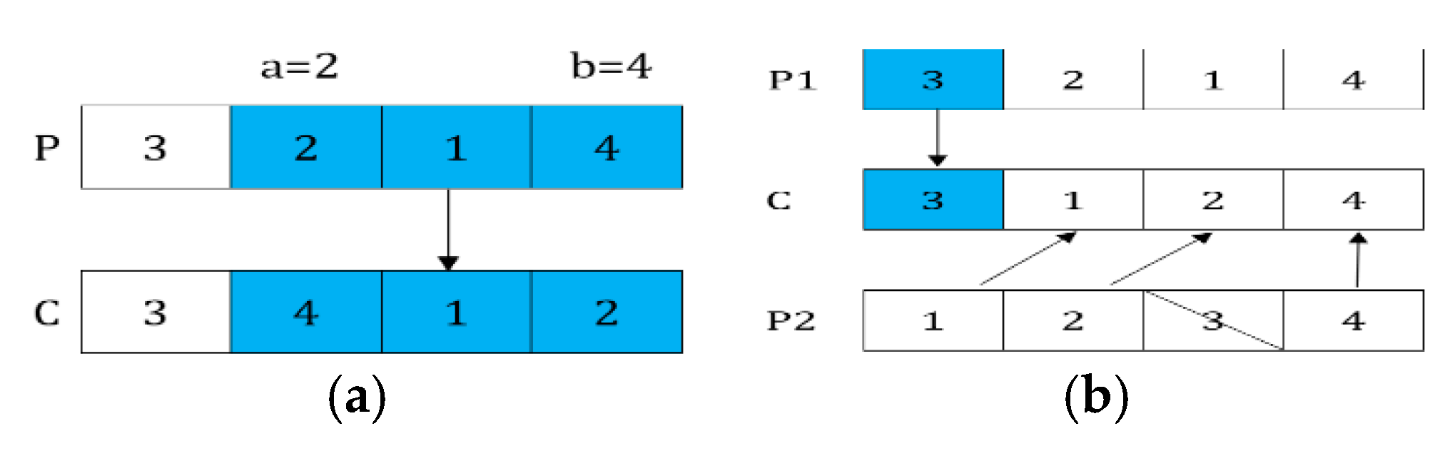
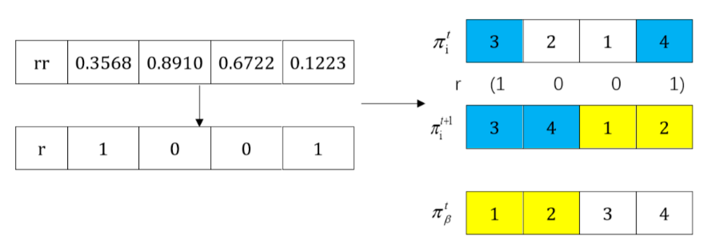
In this paper, the IMOGWO algorithm is designed to solve the green manufacturing collaborative optimization problem of the semiconductor wafer distributed heterogeneous factory. The IMOGWO realizes the rational allocation of jobs to factories and the production scheduling of assigned jobs in factories by adopting heuristic rules DR and the PS decoding method. By designing a reverse learning strategy for the initial population, the fliplr mutation and LOX cross-mutation learning strategies for the leadership level, and the LMOX cross search strategy for the grey wolf individual and randomly selected α wolf, β wolf, δ wolf, and the ω wolf, which enlarges the diversity of the population and improves the quality of the solution. Simulation results demonstrate that the proposed IMOGWO has certain advantages and competitiveness compared with the other three algorithms. The algorithm designed in this paper can find the optimal solution of the scheduling scheme by enlarging the diversity of the population so that the results can jump out of the local optimum. The green scheduling model designed in this paper focuses on the carbon emission indicator. All of these are also applicable to other production scheduling problems, such as distributed flexible job shop green scheduling, distributed uncertain job shop green scheduling, and so on. In the actual semiconductor production, new wafers are continuously put into processing every day, and some operations such as trial processing lead to uncertain processing time of wafers. Therefore, uncertain scheduling in semiconductor wafer manufacturing is our future research direction. In addition, a semiconductor production line may be composed of hundreds of devices, and there may be hundreds of different flowing product types. This is on a very large scale. Therefore, it is imperative to study the scheduling problem of large-scale jobs in semiconductor production.
Lastly, the discussion of more novel technical methods, such as the game theory model, the fuzzy theory, machine learning, and Internet of Things technology to solve the scheduling problem of distributed job shop manufacturing in an effective time is also the focus of our future research.

Author Contributions

J.D. contributed to developing ideas about the framework with algorithms, conducted the experiments, and wrote the paper. C.Y. contributed toward providing guidance for this paper.

Funding

The National Natural Science Foundation of China under Grant Nos. 71840003, Science and Technology Development Project of University of Shanghai for Science and Technology under Grant Nos. 2018KJFZ043, funded this research.

Acknowledgments

The authors would like to thank Hang-Min Cho, Suk-Joo Bae, Jungwuk Kim, and In-Jae Jeong for providing the benchmark instances set to us.

Conflicts of Interest

The authors declare no conflict of interest.

References

  1. Zheng, X.L.; Wang, L.; Wang, S.Y. A novel fruit fly optimization algorithm for the semiconductor final testing scheduling problem. Knowl.-Based Syst. 2013, 57, 95–103. [Google Scholar] [CrossRef]
  2. Jiang, Z.G.; Dong, M.; Tian, P.; Yang, D. Modeling and Simulation of Re-Entrant Semiconductor Wafer Fabrication Lines with PM Using GSPN. Adv. Mater. Res. 2010, 97–101, 2469–2472. [Google Scholar] [CrossRef]
  3. Vargas-Villamil, F.D.; Rivera, D.E.; Kempf, K.G. A hierarchical approach to production control of reentrant semiconductor manufacturing lines. IEEE Trans. Control Syst. Technol. 2003, 11, 578–587. [Google Scholar] [CrossRef]
  4. Kang, Y.H.; Kim, S.S.; Shin, H.J. A scheduling algorithm for the reentrant shop: An application in semiconductor manufacture. Int. J. Adv. Manuf. Technol. 2007, 35, 566–574. [Google Scholar] [CrossRef]
  5. Wang, M.Y.; Sethi, S.P.; Vandevelde, S.L. Minimizing makespan in a class of reentrant shops. Oper. Res. 1997, 45, 702–712. [Google Scholar] [CrossRef]
  6. Wolpert, D.H.; Macready, W.G. No free lunch theorems for optimization. IEEE Trans. Evol. Comput. 1997, 1, 67–82. [Google Scholar] [CrossRef] [Green Version]
  7. Bertel, S.; Billaut, J.C. A genetic algorithm for an industrial multiprocessor flow shop scheduling problem with recirculation. Eur. J. Oper. Res. 2004, 159, 651–662. [Google Scholar] [CrossRef]
  8. Cho, H.M.; Bae, S.J.; Kim, J.; Jeong, I.J. Bi-objective scheduling for reentrant hybrid flow shop using Pareto genetic algorithm. Comput. Ind. Eng. 2011, 61, 529–541. [Google Scholar] [CrossRef]
  9. Li, Z.C.; Qian, B.; Hu, R.; Zhang, C.S.; Li, K. A self-adaptive hybrid population-based incremental learning algorithm for M-machine reentrant permutation flow-shop scheduling. In International Conference on Intelligent Computing Theories; Springer: Berlin/Heidelberg, Germany, 2013; pp. 8–20. [Google Scholar]
  10. Huang, R.H.; Yu, S.C.; Kuo, C.W. Reentrant two-stage multiprocessor flow shop scheduling with due windows. Int. J. Adv. Manuf. Technol. 2014, 71, 1263–1276. [Google Scholar] [CrossRef]
  11. Cho, H.M.; Jeong, I.J. A two-level method of production planning and scheduling for bi-objective reentrant hybrid flow shops. Comput. Ind. Eng. 2017, 106, 174–181. [Google Scholar] [CrossRef]
  12. Modoni, G.E.; Trombetta, A.; Veniero, M.; Sacco, M.; Mourtzis, D. An event-driven integrative framework enabling information notification among manufacturing resources. Int. J. Comput. Integr. Manuf. 2019, 32, 241–252. [Google Scholar] [CrossRef]
  13. Renna, P.; Argoneto, P. A game theoretic coordination for trading capacity in multisite factory environment. Int. J. Adv. Manuf. Technol. 2010, 47, 1241–1252. [Google Scholar] [CrossRef]
  14. Argoneto, P.; Renna, P. Supporting capacity sharing in the cloud manufacturing environment based on game theory and fuzzy logic. Enterp. Inf. Syst. 2014, 10, 1–18. [Google Scholar] [CrossRef]
  15. Xu, Y.; Wang, L.; Wang, S.Y.; Liu, M. An effective hybrid immune algorithm for solving the distributed permutation flow-shop scheduling problem. Eng. Optim. 2014, 46, 1269–1283. [Google Scholar] [CrossRef]
  16. Zhang, H.; Zhao, F.; Sutherland, J.W. Energy-efficient scheduling of multiple manufacturing factories under real-time electricity pricing. CIRP Ann.-Manuf. Technol. 2015, 64, 41–44. [Google Scholar] [CrossRef]
  17. Zhang, G.; Xing, K.; Cao, F. Scheduling distributed flowshops with flexible assembly and set-up time to minimise makespan. Int. J. Prod. Res. 2017, 56, 3226–3244. [Google Scholar] [CrossRef]
  18. Lu, P.H.; Wu, M.C.; Tan, H.; Peng, H.Y.; Chen, C.F. A genetic algorithm embedded with a concise chromosome representation for distributed and flexible job-shop scheduling problems. J. Intell. Manuf. 2018, 29, 19–34. [Google Scholar] [CrossRef]
  19. Fu, Y.P.; Tian, G.D.; Fathollahi-Fard, A.M.; Ahmadi, A.; Zhang, C.Y. Stochastic multi-objective modelling and optimization of an energy-conscious distributed permutation flow shop scheduling problem with the total tardiness constraint. J. Clean. Prod. 2019, 226, 515–525. [Google Scholar] [CrossRef]
  20. Rifai, A.P.; Nguyen, H.T.; Dawal, S.Z.M. Multi-objective adaptive large neighborhood search for distributed reentrant permutation flow shop scheduling. Appl. Soft Comput. 2016, 40, 42–57. [Google Scholar] [CrossRef]
  21. Zhang, C.; Gu, P.; Jiang, P. Low-carbon scheduling and estimating for a flexible job shop based on carbon footprint and carbon efficiency of multi-job processing. Proc. Inst. Mech. Eng. B-J. Eng. 2015, 229, 328–342. [Google Scholar] [CrossRef]
  22. Liu, Q.; Zhan, M.M.; Chekem, F.O.; Shao, X.Y.; Ying, B.S.; Sutherland, J.W. A hybrid fruit fly algorithm for solving flexible job-shop scheduling to reduce manufacturing carbon footprint. J. Clean. Prod. 2017, 168, 668–678. [Google Scholar] [CrossRef]
  23. Nilakantan, J.M.; Li, Z.X.; Tang, Q.H.; Nielsen, P. Multi-objective co-operative co-evolutionary algorithm for minimizing carbon footprint and maximizing line efficiency in robotic assembly line systems. J. Clean. Prod. 2017, 156, 124–136. [Google Scholar] [CrossRef] [Green Version]
  24. Piroozfard, H.; Wong, K.Y.; Wong, W.P. Minimizing total carbon footprint and total late work criterion in flexible job shop scheduling by using an improved multi-objective genetic algorithm. Resour. Conserv. Recycl. 2018, 128, 267–283. [Google Scholar] [CrossRef]
  25. Mirjalili, S.; Mirjalili, S.M.; Lewis, A. Grey Wolf Optimizer. Adv. Eng. Softw. 2014, 69, 46–61. [Google Scholar] [CrossRef] [Green Version]
  26. Mirjalili, S.; Saremi, S.; Mirjalili, S.M.; Coelho, L. Multi-objective grey wolf optimizer: A novel algorithm for multi-criterion optimization. Expert Syst. Appl. 2016, 47, 106–119. [Google Scholar] [CrossRef]
  27. Komaki, G.M.; Kayvanfar, V. Grey Wolf Optimizer algorithm for the two-stage assembly flow shop scheduling problem with release time. J. Comput. Sci. 2015, 8, 109–120. [Google Scholar] [CrossRef]
  28. Lu, C.; Gao, L.; Li, X.Y.; Xiao, S.Q. A hybrid multi-objective grey wolf optimizer for dynamic scheduling in a real-world welding industry. Eng. Appl. Artif. Intell. 2017, 57, 61–79. [Google Scholar] [CrossRef]
  29. Martin, B.; Marot, J.; Bourennane, S. Mixed grey wolf optimizer for the joint denoising and unmixing of multispectral images. Appl. Soft Comput. 2019, 74, 385–410. [Google Scholar] [CrossRef]
  30. Sharma, P.; Sundaram, S.; Sharma, M.; Sharma, A.; Gupta, D. Diagnosis of Parkinson’s disease using modified grey wolf optimization. Cogn. Syst. Res. 2019, 54, 100–115. [Google Scholar] [CrossRef]
  31. Mirjalili, S.M.; Mirjalili, S.Z. Full Optimizer for Designing Photonic Crystal Waveguides: IMoMIR Framework. IEEE Photonic Technol. Lett. 2015, 7, 776–1779. [Google Scholar] [CrossRef]
  32. Snyder, L.V.; Daskin, M.S. A random-key genetic algorithm for the generalized traveling salesman problem. Eur. J. Oper. Res. 2006, 174, 38–53. [Google Scholar] [CrossRef]
  33. Ying, K.C.; Lin, S.W.; Wan, S.Y. Bi-objective reentrant hybrid flowshop scheduling: An iterated Pareto greedy algorithm. Int. J. Prod. Res. 2014, 52, 5735–5747. [Google Scholar] [CrossRef]
  34. Liang, G.X.; Liang, Y.Z.; Chen, H.S. Carbon Audit Toolbox for Small and Medium-Sized Enterprises in Hong Kong; University of Hong Kong: Hong Kong, China, 2010. [Google Scholar]
  35. Tizhoosh, H.R. Opposition-Based Learning: A New Scheme for Machine Intelligence. In Proceedings of the International Conference on Computational Intelligence for Modelling Control and Automation, Vienna, Austria, 28–30 November 2005; IEEE Press: Piscataway, NJ, USA, 2005; pp. 695–701. [Google Scholar]
  36. Deb, K.; Pratap, A.; Agarwal, S.; Meyarivan, T. A fast and elitist multiobjective genetic algorithm NSGA-II. IEEE Trans. Evol. Comput. 2002, 6, 182–197. [Google Scholar] [CrossRef]
  37. Croce, F.D.; Tadei, R.; Volta, G. A Genetic Algorithm for the Job Shop Problem. COMPUT OPER RES. 1995, 22, 15–24. [Google Scholar] [CrossRef]
  38. Chao, L.; Xiao, S.Q.; Li, X.Y.; Gao, L. An effective multi-objective discrete grey wolf optimizer for a real-world scheduling problem in welding production. Adv. Eng. Softw. 2016, 99, 161–176. [Google Scholar] [Green Version]
  39. Deng, J.; Wang, L. A competitive memetic algorithm for multi-objective distributed permutation flow shop scheduling problem. Swarm Evol. Comput. 2017, 32, 121–131. [Google Scholar] [CrossRef]
  40. Minella, G.; Ruiz, R.; Ciavotta, M. A review and evaluation of multi objective Algorithms for the flowshop scheduling problem. INFORMS J. Comput. 2008, 20, 451–471. [Google Scholar] [CrossRef]
  41. Coello, C.A.C.; Pulido, G.T.; Lechuga, M.S. Handling multiple objectives with particle swarm optimization. IEEE Trans. Evol. Comput. 2004, 8, 256–279. [Google Scholar] [CrossRef]
Figure 1. Schematic diagram of the DRHFS problem.
Applsci 09 02879 g001
Figure 2. Scheduling Gantt charts of two factories. (a) Factory 1. (b) Factory 2.
Applsci 09 02879 g002
Figure 3. Schema of the leadership level learning strategies. (a) Fliplr mutation. (b) LOX crossover.
Applsci 09 02879 g003
Figure 4. LMOX cross mode.
Applsci 09 02879 g004
Figure 5. Box-plots of four evaluation indicators for two factories’ test cases.
Applsci 09 02879 g005aApplsci 09 02879 g005b
Figure 6. Box-plots of four evaluation indicators for three factories’ test cases.
Applsci 09 02879 g006
Figure 7. Pareto optimal fronts obtained by each algorithm. (a) 3D map of Pareto fronts. (b) Comparison of Makespan and Total carbon emissions. (c) Comparison of Total tardiness and Total carbon emissions. (d) Comparison of Makespan and Total tardiness.
Applsci 09 02879 g007
Figure 8. Scheduling Gantt charts of jobs processed in two factories. (a) Factory 1. (b) Factory 2.
Applsci 09 02879 g008
Table 1. Mathematical symbols and significance.
Mathematical SymbolsSignificance
n t o t a l Total number of jobs
i Serial number of jobs, i = 1 , 2 , n t o t a l
N i Total number of operations contained in job i
j Operation serial number of jobs i , i , j = 1 , 2 , N i
f Serial number of factories, f = 1 , 2 , F
n f Total number of jobs allocated to the factory f
n f i Serial number of jobs allocated to factory f , n f i = 1 , 2 , n f
F Total number of processing factories
Y i , f 1 indicates that job i is allocated to the factory f , 0 indicates that the job i
is not allocated to the factory for processing
s Total number of stages
l Serial number of stages, l = 1 , 2 , , s
m f l Number of parallel machines with the same speed at stage l of factory f
k Serial number of machines at stage l , k = 1 , 2 , m f l
O i j The j-th operation of job i
T f i j l k Processing time of O i j on machine k at stage l in factory f
P i j f l Processing time of O i j at stage l in factory f
d f i Delivery time of job i processed in factory f
H A large positive number
U f l The set of all operations processed at stage l of factory f , due to the reentrant
characteristics, the same job may appear multiple times in it
P W f l k Processing power of machine k at stage l of factory f
P I f l k Idle power of machine k at stage l of factory f
T f l k I Idle time of machine k at stage l of factory f
T C f p Total carbon emissions from machines processing of factory f
T C f I Total carbon emissions from machines in an idle state of factory f
F e Carbon emissions factor of electric energy
T f l , k , c l o s e The finishing time of machine k at stage l of factory f (the finishing time of the
last operation on the machine)
T f l , k , o p e n The start time of machine k at stage l of factory f (the starting time of the
first operation on the machine)
U R f l k The usage amount of lubricants on machine k at stage l of factory f
T R f l k Effective service time of lubricants on machine k at stage l of factory f
T C f R Total carbon emissions from lubricants used by machines of factory f
F R Carbon emissions factor of lubricants
S f i j The starting time of O i j in factory f
C f i The completion time of job i in factory f
C i j The completion time of O i j
r i j l k 1 indicates O i j , which is processed on machine k at stage l of factory f , 0 indicates
O i j is not processed on machine k at stage l of factory f
Z i j , g h , l k 1 indicates O i j is processed before O g h on machine k at stage l , 0 indicates
O i j is not processed before O g h
T C T f Total carbon emissions from factory f
T D T f Total tardiness of jobs processed in factory f
C max Make span of all jobs
T C T Total carbon emissions
T D T Total tardiness
Table 2. Objective functions and constraints.
ExpressionSignificance
f 1 = min ( C max ) minimizing the make span
f 2 = min ( T C T ) = min ( f = 1 F T C T f ) minimizing the total carbon emissions
f 3 = min ( T D T ) = min ( f = 1 F T D T f ) minimizing the total tardiness
T C T f = T C f p + T C f I + T C f R Total carbon emissions from factory f
T D T f = i = 1 n f max ( 0 , C f i d f i ) ) Total tardiness of jobs processed in factory   f
Y i , f r i j l k ( S f i j + T f i j l k ) Y i , f r i , j + 1 , l , k S f i , j + 1 Indicates the completion time of O i j must be earlier
i , j , l , l a n d   l l than the starting time of O i j + 1
k = 1 m f l r i j l k = 1 f , i , j , k , l , O i j U i Indicates any operation can be processed on only one machine in the corresponding stage
f = 1 F Y i , f = 1 i , f Indicates one job can only be assigned to one factory for processing
H × Y i , f ( 2 r i j l k r g h l k ) + H × Y g , f ( 1 Z i j , g h , l k ) + ( S f g h S f i j ) T f i j l k Indicates each machine in any stage can only process at most one operation at the same time
f , i , g , j , h , i g , O i j U l , O g h U l
H × Y i , f ( 2 r i j l k r i j l k ) + H × Y i , f ( 1 Z i j , i j , l k ) + ( S f i j S f i j ) T f i j l k
f , i , k , l , j < j , O i j U l , O i j U l
f = 1 F l = 1 s k = 1 m f l i = 1 n t o t a l j = 1 N i Y i , f r i j l k ( S f i j + T f i j l k ) C max f , i , j , k , l Indicates the definition of make span
T C f P = l = 1 s k = 1 m f l i = 1 n j = 1 N i Y i , f r i j l k F e P W f l k T f i j l k Indicates the total carbon emissions generated from machines processing in factory f
T C f I = l = 1 s k = 1 m f l F e P I f l k T f l k I Indicates the total carbon emissions generated from
machines in an idle state in factory f
T C f R = l = 1 s k = 1 m f l T f l , k , c l o s e T f l , k , o p e n T R f l k U R f l k F R Indicates the total carbon emissions generated from the use of lubricants in factory f
Table 3. Processing time and delivery time of each job.
Factory 1 (Factory 2)
JobsDelivery TimeFirst ProcessingFirst ReentrySecond Reentry
Stage 1Stage 2Stage 3Stage 1Stage 2Stage 3Stage 1Stage 2Stage 3
Job113.2(11.1)1(2)2(2)2(2)1(0)2(2)1(2)2(0)2(2)1(1)
Job211.8(14.2)2(2)2(0)2(3)1(2)2(1)2(2)1(1)2(2)2(1)
Job315.6(15.1)1(2)1(0)2(2)0(1)2(2)1(0)2(2)2(2)1(0)
Job411.5(13.4)2(2)1(1)2(2)2(2)1(0)1(1)1(1)2(3)2(1)
Table 4. Average processing time of each job in two factories.
Factory 1Factory 2
job199.5
job2108.5
job37.57.5
job49.58.5
Table 5. Parameters and values of algorithms.
ParameterValue
Number of jobsAn integer follows uniform distribution between [10,20]
Number of stagesAn integer follows uniform distribution between [5,10]
Number of re-entriesAn integer follows uniform distribution between [1,2]
Number of factories2\3
Crossover probability (NSGA-II)0.8
Mutation probability (NSGA-II)0.3
Number of cycles of algorithms100
Number of populations50
Archive size (MOGWO)50
Gamma (MOGWO)2
Alpha (MOGWO)0.1
nGrid (MOGWO)10
Beta (MOGWO)4
Processing power of machines at each stageAn integer follows uniform distribution between [5, 8]
Idle power of machines at each stageAn integer follows uniform distribution between [1, 5]
Effective service time of lubricants on the machines at each stageAn integer follows uniform distribution between [4, 6]
The amount of lubricants used on the machines at each stageAn integer follows uniform distribution between [0.2, 0.4]
Carbon emissions factor of electric energy0.6747 kgCO2/kw·h
Carbon emissions factor of lubricants2.85 kgCO2/L
Remarks: Power unit: kw/h, effective service time unit of lubricants: h, usage unit of lubricants: L.
Table 6. Experimental results comparison of four algorithms with two factories.
Test ExampleIMOGWOMODGWOMOGWONSGA-II
AvgMinAvgMinAvgMinAvgMin
(Max)(Max)(Max)(Max)
ProblemSP0.25250.05530.29650.14850.17170.12370.33740.0349
01-01GD0.06170.00660.18170.08660.06250.0260.08030.03
IGD0.17350.04690.41750.31860.18150.06050.24750.1127
Ω43%58%3%15%32%46%22%63%
ProblemSP0.10810.08520.56390.31110.13920.07660.14210.0941
01-11GD0.01650.00960.17450.0590.03760.01590.03280.0182
IGD0.07010.04190.42090.23810.1350.07880.14140.0927
Ω61%65%3%25%17%28%19%24%
ProblemSP0.27230.11870.59810.13860.25090.13690.37180.2188
02-01GD0.10570.04840.19490.08270.11210.02980.1370.088
IGD0.26860.16610.50290.29890.270.12820.3040.1127
Ω56%71%5%18%26%44%13%29%
ProblemSP0.22460.08260.60760.28110.2510.12070.26780.1359
02-11GD0.03230.01570.22120.07560.06640.02570.13310.0503
IGD0.10080.00020.44920.24660.21010.0980.31670.1159
Ω65%88%3%14%16%35%16%22%
ProblemSP0.2180.14810.42890.13990.34110.15830.3580.2749
03-01GD000.17510.1240.11910.06890.15380.0608
IGD000.46730.23450.35180.23920.36820.2191
Ω89%100%2%12%5%25%4%20%
ProblemSP0.28980.21410.43570.37580.34580.19490.51620.2052
03-11GD0.11740.0570.199700.13990.08990.12370.0519
IGD0.210.13440.44240.08190.33530.27750.29830.1487
Ω55%81%31%83%4%11%10%19%
ProblemSP0.22010.13640.48880.1970.16350.1120.34260.135
04-01GD0.04440.02390.18710.08210.0430.02630.0780.0289
IGD0.15910.03280.41770.24620.17160.12390.21980.1079
Ω50%88%10%23%21%33%19%27%
ProblemSP0.1870.08760.36470.1770.26290.13040.29580.2185
04-11GD0.03690.01010.20490.08250.0530.0380.04620.0297
IGD0.13450.02930.45680.21450.190.12680.16590.1155
Ω43%63%8%28%34%58%16%35%
ProblemSP0.32260.15430.26860.04510.30250.11960.32590.178
05-01GD0.048900.20350.07960.09070.03150.11040.0415
IGD0.135700.47260.3460.24070.12640.22040.0778
Ω70%100%5%10%2%10%23%75%
ProblemSP0.22020.09560.35950.06410.32460.15320.320.1056
05-11GD0.088100.18780.12010.1280.06360.1120.0509
IGD0.20800.44010.2860.31610.24970.3470.2215
Ω74%100%16%50%0%0%10%33%
ProblemSP0.24160.1110.36610.04890.22250.12560.24720.145
06-01GD0.05540.02050.15970.07680.05230.02410.07650.0425
IGD0.19130.10460.37930.22550.21730.16010.24710.1956
Ω63%86%6%25%10%13%21%43%
ProblemSP0.1110.07070.31710.14020.11630.07450.18470.0703
06-11GD0.01660.01220.08510.05210.02790.01990.04950.0266
IGD0.08360.04080.30890.19640.14820.12270.19170.1246
Ω64%72%7%15%13%29%30%100%
MeanSP0.22230.11330.42460.17230.2410.12720.30910.1514
GD0.0520.0170.18130.07680.07770.03830.09440.0433
IGD0.14460.0450.43130.24440.23060.14930.25570.1371
Ω62%81%8%27%15%28%17%41%
Table 7. Wilcoxon signed rank test (two factories).
IndicatorSproblem 01-06(01 Problem) sig (p < 0.05)Sproblem 01-06(11 Problem) sig (p < 0.05)
MODGWO MOGWONSGA-IIMODGWO MOGWONSGA-II
PSigPSigPSigPSigPSigPSig
SP0.005Y0.506N0.035Y0.000Y0.013Y0.003Y
GD0.000Y0.111N0.011Y0.000Y0.003Y0.002Y
IGD0.000Y0.025Y0.000Y0.000Y0.000Y0.000Y
Ω 0.000Y0.000Y0.000Y0.000Y0.000Y0.000Y
Table 8. Experimental results’ comparison of four algorithms with three factories.
Test ExampleIMOGWOMODGWOMOGWONSGA-II
AvgMinAvgMinAvgMinAvgMin
(Max)(Max)(Max)(Max)
ProblemSP0.11420.08570.38640.01560.14160.07520.21210.1651
01-01GD0.01610.01190.12420.07470.02480.01950.0460.0279
IGD0.06330.03640.38250.24990.11310.07340.19710.133
Ω57%69%3%23%25%29%15%29%
ProblemSP0.12970.08570.49870.02130.16510.11470.19850.0992
01-11GD0.01620.01050.12120.09130.02510.02090.03730.0204
IGD0.07360.05520.3730.24990.1250.06870.16160.1502
Ω64%75%2%8%19%24%15%21%
ProblemSP0.13220.08890.33420.12550.18250.12290.18510.1131
02-01GD0.04070.01160.13810.06670.06470.03070.07330.0376
IGD0.1540.06970.37490.28690.19460.07340.25310.1764
Ω63%86%11%40%9%20%17%30%
ProblemSP0.14270.08710.4470.15110.1830.09180.18880.1255
02-11GD0.04580.00410.17250.06670.07340.02640.07260.0259
IGD0.15680.00930.43620.29130.24910.12170.25640.1182
Ω69%92%7%44%8%22%15%34%
ProblemSP0.37870.32480.5050.27970.15580.10120.41550.2217
03-01GD0.047300.28650.18540.09670.08180.16070.0287
IGD0.069600.54120.38690.23080.16350.29850.1114
Ω67%100%0%0%0%0%23%84%
ProblemSP0.85240.30060.87640.79210.72870.53620.15010.0899
03-11GD000.36330.21350.31440.30220.04120.0122
IGD000.61560.49860.75330.54730.11260.0942
Ω100%100%0%0%0%0%0%0%
ProblemSP0.13430.06370.25870.06720.13720.07050.22210.1085
04-01GD0.02710.00630.15270.11950.03750.02230.07480.0362
IGD0.09410.02560.35220.2680.15470.07110.18530.1428
Ω64%70%3%15%23%41%10%30%
ProblemSP0.11420.06570.37360.11760.190.12010.1650.1108
04-11GD0.01750.01110.12690.07130.03460.01980.03450.025
IGD0.07130.03570.40120.2590.20110.13720.14010.1148
Ω48%80%3%10%33%54%16%28%
ProblemSP0.2820.1190.35470.16090.35440.08990.24210.1068
05-01GD0.046300.15130.07110.09890.07250.11040.0163
IGD0.152400.39570.23980.27710.15570.29310.0808
Ω55%100%8%44%4%11%34%69%
ProblemSP0.40940.13020.3130.24240.22160.13240.32770.0815
05-11GD0.16570.12680.2420.05080.22170.13280.21960.1165
IGD0.38370.2320.48610.13990.46320.30610.49260.3112
Ω32%73%48%75%8%20%13%30%
ProblemSP0.15860.08010.37240.15420.19570.12060.340.1482
06-01GD0.02090.00860.15420.06820.0560.03690.06580.0486
IGD0.08450.01550.44640.2760.20970.15530.21070.1686
Ω67%93%0%0%15%33%17%35%
ProblemSP0.10460.06220.27350.19470.11350.07350.11370.0439
06-11GD0.01720.01030.1260.0590.01810.00920.03180.0145
IGD0.06790.04550.28370.21530.08980.05330.12170.0813
Ω69%77%5%13%12%20%15%25%
MeanSP0.24610.12450.41610.19350.23080.13740.23010.1179
GD0.03840.01680.17990.09490.08880.06460.08070.0342
IGD0.11430.04370.42410.28010.25510.16060.22690.1402
Ω63%85%5%13%13%23%16%35%
Table 9. Wilcoxon signed rank test (thre factories).
IndicatorSproblem01-06(01 Problem) Sig (p < 0.05)Sproblem01-06(11 Problem) Sig (p < 0.05)
MODGWOMOGWONSGA-IIMODGWOMOGWONSGA-II
PSigPSigPSigPSigPSigPSig
SP0.000Y0.866N0.006Y0.000Y0.732N0.874N
GD0.000Y0.000Y0.000Y0.000Y0.017Y0.001Y
IGD0.000Y0.000Y0.000Y0.000Y0.003Y0.000Y
Ω 0.000Y0.000Y0.000Y0.000Y0.000Y0.000Y
Table 10. Relevant parameters in factory 1.
ParametersValues
Number of parallel machines at each stage[1, 1, 1, 1, 1, 2, 2, 1], A total of 10 machines
Processing time of each operationAn integer follows uniform distribution between [1, 10]
Processing power of machines at each stage[6, 7, 5, 5, 6, 6, 5, 5] (Unit: kw/h)
Idle power of machines at each stage[5, 3, 4, 2, 2, 1, 2, 2] (Unit: kw/h)
Effective service time of lubricants on the machines at each stage[5.1, 4.8, 4.9, 5.0, 5.3, 4.4, 4.9, 5.9] (Unit: h)
The amount of lubricants used on the machines at each stage[0.34, 0.27, 0.25, 0.37, 0.22, 0.28, 0.34, 0.37] (Unit: L)
Delivery time of each job[69.5520, 66.6540, 49.2660, 89.8380, 89.8380, 84.0420, 73.8990, 56.5110, 65.2050, 73.8990, 56.5110, 92.7360, 76.7970, 73.8990, 71.0010] (Unit: min)
Table 11. Relevant parameters in factory 2.
ParametersValues
Number of parallel machines at each stage[1, 2, 1, 2, 1, 2, 1, 1], A total of 11 machines
Processing time of each operationAn integer follows uniform distribution between [1,10]
Processing power of machines at each stage[8, 8, 8, 5, 8, 7, 8, 6] (Unit: kw/h)
Idle power of machines at each stage[1, 3, 1, 5, 1, 4, 4, 3] (Unit: kw/h)
Effective service time of lubricants on the machines at each stage[5.9, 4.4, 4.7, 4.1, 5.7, 4.4, 5.9, 5.1] (Unit: h)
The amount of lubricants used on the machines at each stage[0.23, 0.33, 0.36, 0.36, 0.29, 0.30, 0.32, 0.22] (Unit: L)
Delivery time of each job[88.5311, 107.1938, 108.0180, 139.7903, 93.3949, 186.1302, 110.8196129.5210, 117.1030, 116.3252, 123.3349, 92.1824, 180.2294, 142.0430, 143.8744] (Unit: min)
Table 12. Pareto solutions and corresponding jobs-to-factories allocation scheme (part).
SerialTotal Carbon EmissionsTotal TardinessMake SpanScheduling Scheme
Number/minFactory 1Factory 2
1107.5274161.64751408-13-15-12-7-2-11-14-61-3-9-10-5-4
278.4246192.9531328-13-7-10-15-2-5-3-14-11-6-4-19-Dec
374.0678188.9521348-1-7-14-13-10-2-5-3-6-11-15-49-Dec
473.9144228.4411108-13-7-11-6-5-14-1-3-15-2-10-412-Sep
571.6828310.7031188-11-14-3-1-6-2-5-10-15-13-7-49-Dec
673.1589191.2991338-10-14-1-15-13-7-2-3-11-5-4-69-Dec
772.1279277.5421098-13-7-11-6-5-1-2-10-3-15-4-149-Dec
874.8563213.0341232-8-13-7-11-5-14-6-4-10-1-15-39-Dec
973.2467216.0531162-10-8-1-13-7-11-5-14-6-3-15-49-Dec
1073.3567227.4411118-13-7-11-6-5-2-10-1-3-15-4-149-Dec

