Influence of Variation/Response Space Complexity and Variable Completeness on BP-ANN Model Establishment: Case Study of Steel Ladle Lining

Abstract

Artificial neural network (ANN) is widely applied as a predictive tool to solve complex problems. The performance of an ANN model is significantly affected by the applied architectural parameters such as the node number in a hidden layer, which is largely determined by the complexity of cases, the quality of the dataset, and the sufficiency of variables. In the present study, the impact of variation/response space complexity and variable completeness on backpropagation (BP) ANN model establishment was investigated, with a steel ladle lining from secondary steel metallurgy as the case study. The variation dataset for analysis comprised 160 lining configurations of ten variables. Thermal and thermomechanical responses were obtained via finite element (FE) modeling with elastic material behavior. Guidelines were proposed to define node numbers in the hidden layer for each response as a function of the node number in the input layer weighted with the percent value of the significant variables contributing above 90% to the response, as well as the node number in the output layer. The minimum numbers of input variables required to achieve acceptable prediction performance were three, five, and six for the maximum compressive stress, the end temperature, and the maximum tensile stress.

1. Introduction

Artificial neural network (ANN), a technique for artificial intelligence and machine learning, is often applied as a tool to deal with nonlinear problems and offer predictions in civil engineering [1,2,3,4], material science [5,6], etc. The extension of its applications into the iron and steel industry is also reported [7,8,9,10,11].

Architecture establishment of a suitable ANN model is still challenging in the definition of the layer number and node number in the respective layer. Generally, a three-layer ANN model is sufficient to build the relations among variables and responses [12]. Therefore, the determination of the proper node number in the single hidden layer is the key issue.

Table 1. Literature study of rules to define the node number in the hidden layer.

Research Field	Ntrain	Ni	Ntrain/Ni	No	Nh Range	Number of Trials	Optimal Nh	Equation (1)	Equation (2)	Equation (3)	Equation (4)	Equation (5)	Equation (6)
Erosion of beaches [13]	105	3	35	15	1–20	20	3	[5, 15]	[4, 15]	4, 5	26, 27	19, 20	17
Energy conservation in old buildings [14]	66	7	9.4	1	4–15	12	15	[3, 13]	[2, 13]	2, 3	8, 9	12, 13	5, 6
Power output [15]	–	5	–	1	1–11	11	7	[3, 13] Δ	[2, 13] Δ	2, 3	–	–	4, 5
Phytoremediation of palm oil secondary effluent [16]	30	3	10	2	1–15	15	13	[3, 13] Δ	[2, 13] Δ	2, 3	7, 8	7, 8	4
Adsorption of metal ions [17]	13	3	4.3	3	1–15	15	14	[4, 14] Δ	[3, 14] Δ	2, 3	3, 4	6, 7	5
Extraction of sensing information [18]	500	100	5	1	11–20	10	19	[11, 20] *	[10, 20] Δ	10, 11	4, 5	72, 73	67, 68
Lithology identification for shale oil reservoir [19]	220	11	20	4	7–11	5	10	[4, 14] *	[3, 14] Δ	3, 4	18, 19	22, 23	11, 12
Moisture content prediction in paddy drying process [20]	–	3	–	1	2–12	11	2	[3, 12]	[2, 12] *	2 Δ	–	–	3
Corn variety identification [21]	–	10	–	3	3–14	12	8	[4, 14] Δ	[3, 14] *	3, 4	–	–	9, 10
Mechanical behavior of mortar [22]	30	6	5	1	1–9	9	2	[3, 13]	[2, 13] Δ	2, 3 *	4, 5	8, 9	5
Extraction of phenolic compounds [23]	12	3	4	1	1–3	3	2	[3, 12]	[2, 12] Δ	2 Δ	3 *	5, 6	3
Damage pattern of structural systems [24]	113	10	11.3	4	17, 18	2	17	[4, 14]	[3, 14]	3, 4	10, 11	17, 18 *	10, 11
Ntrain is the dataset size for training.
Ni, Nh, No are the nodes numbers in the input, hidden, and output layer, respectively.
– Data are not available in the literature.
* The rule was used to define nodes number in the hidden layer by the authors in their publication.
Δ Rules that optimal Nh are coincident with.

lists the publications on the optimization of the single hidden layer node number. To seek an optimal one, many applied the trial and error method in a diverse range of the node numbers [13,14,15,16,17]; whilst others merely followed the rules of thumb proposed in the literature [18,19,20,21,22,23,24], and the application of rules can significantly reduce the number of trials. Six selected rules of thumb [18,19,20,21,22,23,24,25] used in the respective publication are given below and indicated in Table 1 with an asterisk. The node number or number range for each study was calculated according to the six rules of thumb and compared to the optimal hidden layer node number determined in the respective study. It is evidently shown that the extended applications of six empirical equations into other fields are far less satisfying. Equations (1) and (2) show more robust applications, yet they yield a rather larger number for trials.

N_h = (N_i + N_o)^1/2 + a, a ϵ [1, 10]

(1)

N_h = (N_i + N_o)^1/2 + a, a ϵ [0, 10]

(2)

N_h = (N_i × N_o)^1/2

(3)

N_h = N_train/(N_i + 1)

(4)

$$N_h= 1/2 \left(N_i+N_o\right)+N_{train}^{1/2}$$

(5)

N_h = 2/3 (N_i) + N_o

(6)

where, N_i, N_h, and N_o are the node numbers in the input, hidden, and output layer, N_train is the dataset size for training, and a is an empirical integer not larger than 10.

Several reasons contribute to the diverse results of the hidden layer node number optimization with the six rules of thumb. One is the problem nature or complexity. As shown in Table 1, the optimal values of erosion of beaches and energy conservations in old buildings are out of the range defined by the empirical equations. One empirical equation may show consistent performance for the problems within similar complexity. For instance, the prediction of Equation (3) for beach erosion [13] is rather close to the optimal value that was used as the rule of thumb in the study of the mechanical behavior of mortar [22]. The second reason is the quality of the dataset for training. The optimal training dataset size was suggested to be ten times larger than the total number of weights and biases [12]. A steel ladle lining study showed that the dataset size could be 16 times larger than the variable number in the input layer, in the case of a well-distributed dataset in variation/response spaces [26]. Table 1 also shows the size of the dataset for training and the ratio of the training dataset size to the number of variables quoted in literature. Mostly, the information of dataset quality is missing and insufficient dataset size relative to the variable number could be expected. Finally, the sufficiency of important variables or factors, i.e., the variable completeness, in the problem definition shall also be taken into account.

The present paper investigates the influence of variation/response space complexity and variable completeness on the required node numbers for a three-layer backpropagation (BP)-ANN model using steel ladle lining as a case study. A representative dataset was obtained by a sample screening approach applying multiple orthogonal arrays [26]. The dataset contains 160 samples constituted by ten variables and three responses. The first part of the paper examines the prediction performance of three-layer BP-ANN models with various node numbers in the hidden layer, to reveal the correlation among the node numbers of input and output layers, the ratio of the number of variables contributing above 90% to the response to the total number of variables, and the node number of the hidden layer for each response. In the second part, several combinations of variables were tested as inputs for given three-layer BP-ANN models to assess the influence of the ratio of input variables to the total number of variables on the prediction performance.

2. Methodology

2.1. Numerical Experiments

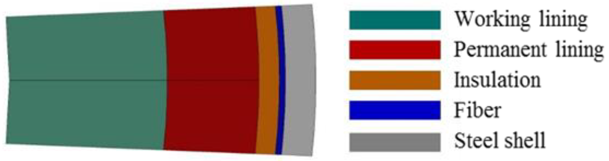
2.1.1. Lining Concept Design

Ten main variables prescribing steel ladle linings were selected for numerical experiments design. These variables (

Table 2. Geometrical and material property variables of steel ladle [26].

	Variables	Range of Variable Values	Label of Variables
Thickness (m)	Working lining	0.03–0.27	A
	Permanent lining	0.05–0.14	B
	Insulation	0.003–0.042	C
	Steel shell	0.015–0.035	J
Thermal conductivity (Wm−1K−1)	Working lining	1.5–10.5	D
	Permanent lining	1.0–10.0	E
	Insulation	0.05–1.55	F
Young’s modulus (GPa)	Working lining	25–115	G
	Permanent lining	5–110	H
	Insulation	0.1–39.1	I

) were the thicknesses of refractory linings and the steel shell, thermal conductivity and Young’s modulus of lining materials. The dataset of lining configurations was designed by a sample screening approach developed in the previous work [26], applying five mixed-level orthogonal arrays L₃₂ (4⁹ × 2¹) with nine four-level variables, and a two-level variable for the thickness of the steel shell. This gives a total amount of 160 experiments (See Supplementary Material).

2.1.2. Finite Element Models

Finite element (FE) modeling was carried out with a commercial software ABAQUS to obtain the thermal and thermomechanical responses of the steel ladle considering elastic material behavior. The simplified two-dimensional numerical model representing a horizontal cut through the slag-line position in the upper part of the steel ladle is depicted in Figure 1. The model was composed of five layers, namely, a two-half brick working and permanent lining, an insulation lining, a fiberboard, and a steel shell. There was 0.4 mm circumferential expansion allowance between bricks. The modeling considered the first process cycle of the steel ladle, which included preheating the hot face of the working lining to 1100 °C over 20 h, tapping the steel melt of 1600 °C into the ladle, transport and refining for 95 min, and a 50 min idle period. The radial displacement of linings was free and the circumferential one was constrained by a symmetry condition. The temperature-dependent surface film condition function in ABAQUS was applied to define the heat transfer between both the melt and the hot face of the working lining and the steel shell and the ambient atmosphere. A heat flux crossed the interfaces between linings, and radiation and convection were allowed by applying a heat transfer coefficient. From 160 numerical experiments, the end temperature and the maximum tensile stress at the cold end of the steel shell and the maximum compressive stress at the hot face of the working lining were obtained from FE modeling.

2.2. BP-ANN Modeling

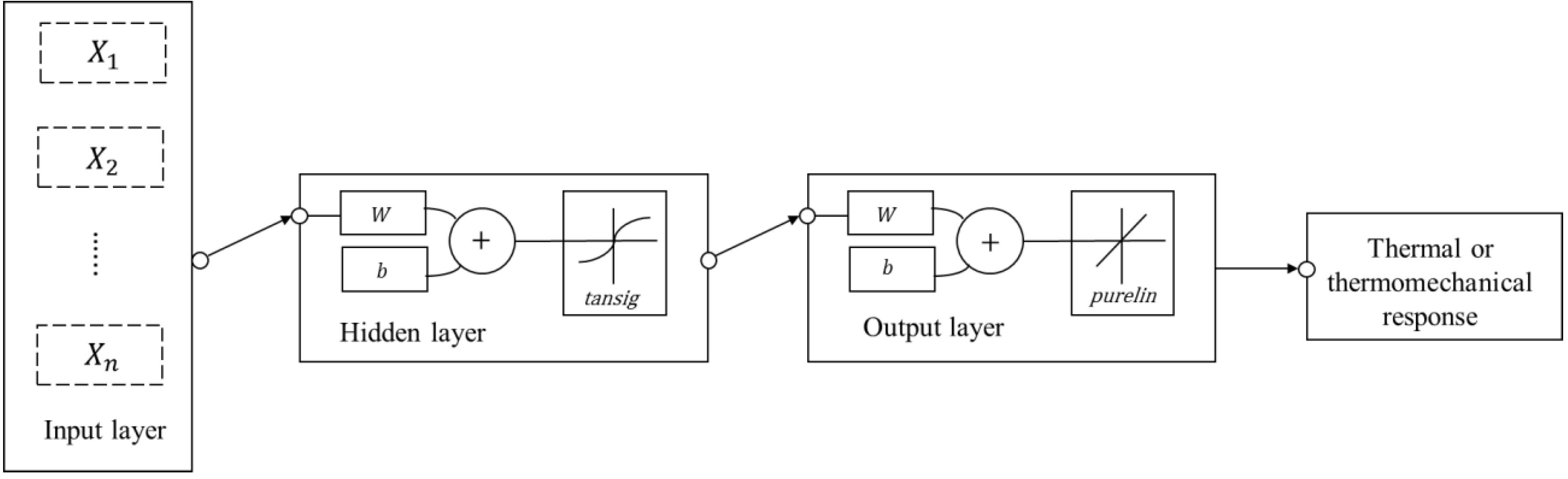
2.2.1. BP-ANN Architecture

A three-layer BP-ANN model, which includes one input, one hidden, and one output layer, is one of the most popular ANN models. The input variables are introduced to the input layer by a vector (X). A summation for each node in the hidden layer is conducted by multiplying input values with their respective weights (W) plus a bias (b) constant. The summation is processed by an activation function and transferred to the hidden layer. The same procedure is carried out between the hidden and output layers. The predicted values at the output layer are compared with the target values and errors are calculated. Weights and biases among layers are updated iteratively until a user-defined performance goal is achieved. The schematic of a three-layer ANN model is demonstrated in Figure 2.

In the present study, two groups of three-layer BP-ANN models were employed to investigate the optimal range of the node numbers in the hidden layer for individual response and the influence of the ratio of input variables to the ten variables (indicating the variable completeness) on the prediction performance. In the first group, there were ten nodes in the input layer, one node in the output layer, and the node number in the hidden layer varied from 1 to 20. The preferable node number range in the hidden layer for each response was proposed afterward. In the second group, different combinations of significant input variables for the individual response were selected according to the ANOVA results of the previous work [27] and listed in

Table 3. Variable combinations of each response for backpropagation (BP)-ANN models.

Response	Number of Input Variables	Variable Labels	Contribution to Response (%)
Compressive stress	1	G	93
	2	G, J	96
	3	G, J, D	98
	10	A–J	100
End temperature	3	A, D, F	71
	4	A, D, F, C	89
	5	A, D, F, C, E	94
	10	A–J	100
Tensile stress	4	F, G, D, J	71
	5	F, G, D, J, C	78
	6	F, G, D, J, C, H	85
	7	F, G, D, J, C, H, I	91
	10	A–J	100

with their contribution summations to the response. For each combination, several BP-ANN models were employed with the node number of the hidden layer in the range proposed from the first group tests. For both groups, the activation function between the input and hidden layers was a hyperbolic tangent sigmoid function [28], and a linear function was applied between the hidden and output layers. The training algorithm was the gradient descent with momentum and adaptive learning rate [28]. Training was terminated by reaching any defined criterion, for instance, a maximum number of epochs (10,000), the minimum performance gradient (10⁻⁵), or a minimum target error (0).

Before starting the network modeling, input variables were normalized to a scale of 0.1–0.9 to mitigate the influence of magnitudes. The normalization of a variable (X_i) can be carried out according to Equation (7).

$$X_i= \frac{0.1x_{max}-0.9x_{min}+0.8x_i}{x_{max}-x_{min}}$$

(7)

where x_max and x_min are the maximum and minimum values of the variable x.

2.2.2. Performance Assessment of BP-ANN Models

The responses were predicted by the leave-one-out (LOO) cross-validation method, i.e., one simulation result was left for testing and the remaining results were used for training. Three quantities were used to quantitatively assess the performance of the BP-ANN models. They were the maximum relative error of all testing results (RE_MAX), mean relative error (MRE), and coefficient of determination (B) calculated by the following equations:

$$RE\_MAX=Max\left(\frac{\left|d_i-y_i\right|}{d_i}\right)$$

(8)

$$MRE=\frac{1}{n}\sum _{i=1}^n\frac{\left|d_i-y_i\right|}{d_i}$$

(9)

$$B=1-\frac{{\sum }_{i=1}^n{\left(d_i-y_i\right)}^2}{{\sum }_{i=1}^n{\left(d_i-\overline{d}\right)}^2}$$

(10)

where n is the total number of testing experiments, d_i is the FE-simulated value of the ith testing experiment, $\overline{d}$ is the mean FE-simulated value of all the testing experiments, y_i is the BP-ANN predicted value of the ith testing experiment with the LOO method.

3. Results and Discussion

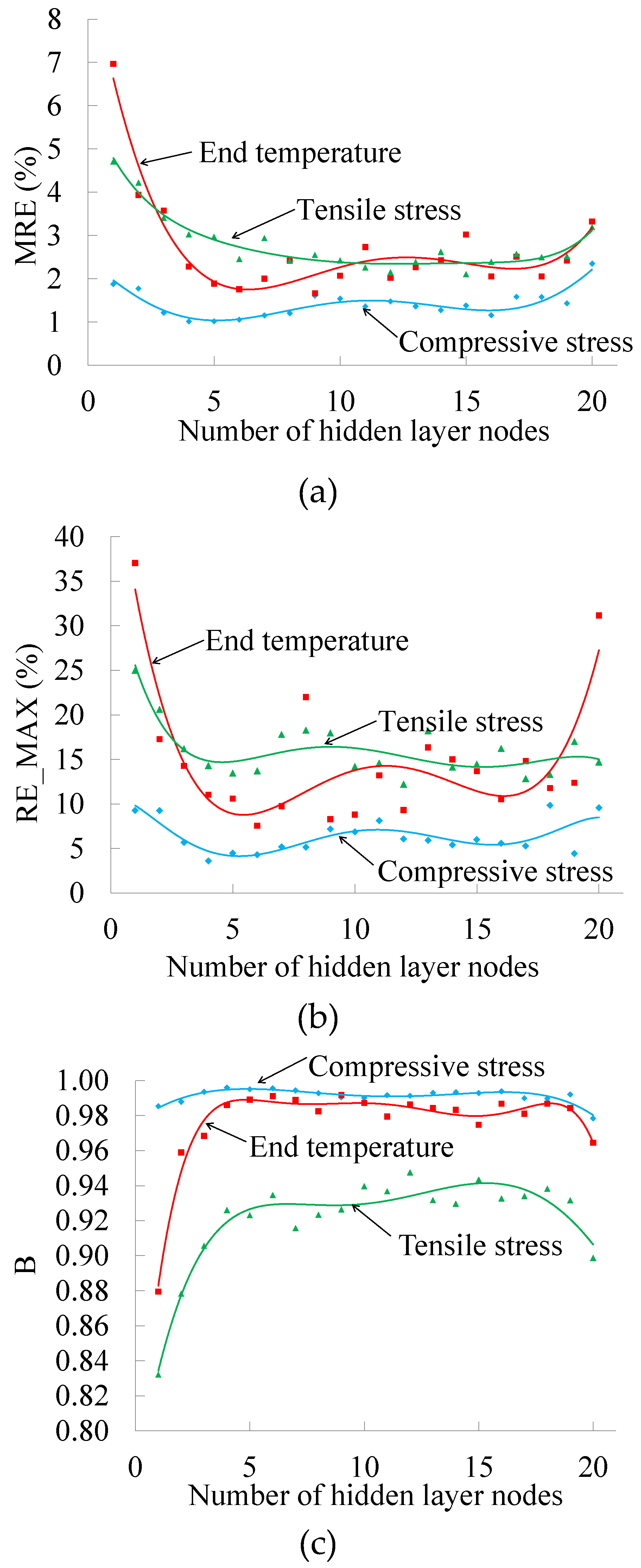
3.1. Influence of Variation/Response Space Complexity on BP-ANN Model Establishment

The relation between the complexity of variation/response space and the node number in the hidden layer for each response was revealed. Except the 32 experiments acting as boundaries, the remaining 128 experiments were tested by leave-one-out cross-validation. The node number in the hidden layer was varied from 1 to 20 for each response. The assessment of the prediction performance is shown in Figure 3. Lower RE_MAX and MRE and larger B are preferable.

Figure 3 shows that the performance is significantly improved by increasing the node number in the hidden layer to seven. However, the performance is oscillatory with further increasing node number; the larger number of nodes may lead to over-fitting and affect the generalization capability. For instance, when the node number is 20, the mean relative errors increase for all three responses; the coefficients of determination decrease; the maximum relative error for end temperature is quite high. Furthermore, it shows that each response has different optimal ranges.

Considering the particular behavior of each response, error criteria were specifically defined for each response and a preferable range of the node number in the hidden layer was proposed for each response (

Table 4. Optimal node number range in the hidden layer for each response according to predefined error criteria.

Response	RE_MAX (%)	MRE (%)	${\mathit{N}}_{\mathit{h}}$ Range
Compressive stress	5	1.5	[4, 6]
End temperature	11	2	[5, 7]
Tensile stress	15	2.5	[10, 12]

). The range was 4–6 for the maximum compressive stress at the hot face of the working lining, 5–7 for the end temperature of the steel shell, and 10–12 for the maximum tensile stress at the cold end of the steel shell. These ranges can be correlated with the node numbers in the input and output layers, as shown in

Table 5. Correlation between PF and node numbers in the input and output layers.

Response	PF	${\mathit{N}}_{\mathit{h}}$
		Lower Boundary	Upper Boundary
Maximum compressive stress	10	$\frac{3}{10}{N}_i+N_o$	$\frac{5}{10}{N}_i+N_o$
End temperature	50	$\frac{4}{10}{N}_i+N_o$	$\frac{6}{10}{N}_i+N_o$
Maximum tensile stress	70	$\frac{9}{10}{N}_i+N_o$	$\frac{11}{10}{N}_i+N_o$

. The number of variables that contribute more than 90% to the response was used to calculate the PF value, which represents the variation/response complexity. This number was divided by ten (the total number of variables) and multiplied by 100, which gave a PF value in percent. Table 5 shows that the PF equaled 10, 50, and 70 for the maximum compressive stress, end temperature, and maximum tensile stress, respectively. Therefore, the relation between the complexity of the variation/response space and the node number in the hidden layer can be associated with the PF and the node numbers in the input and output layers explicitly. Two equations were deduced from Table 5.

Lower boundary: N_h = AN_i + N_o

(11)

Upper boundary: N_h = (A + 0.2) N_i + N_o

(12)

where A is a function of the PF, N_i, N_h, and N_o are the node numbers in the input, hidden, and output layers, respectively.

The relation between A and PF was fitted by an exponential equation (Equation (13)) as shown in Figure 4. Equations (11)–(13) provide guidelines to define node number in the hidden layer for a steel ladle system based on PF and node numbers in the input and output layers.

$$A=f\left(PF\right)= 0.2982-0.001242 (1-e^{0.08836 * PF)}$$

(13)

The above established guidelines were applied to validate the optimal node numbers in several publications [15,19,20,22,23,24], which fall under the topics of temperature, mechanical behavior, and material development. The calculations of the node number range of the hidden layer for these publications were performed with PF values of 10 and 70, respectively. A wide range was created by the lower boundary value with PF values of 10 and the upper boundary value with PF values of 70. The optimal node numbers in the hidden layer obtained from literature and the calculated ranges from proposed guidelines are given in

Table 6. Comparison of optimal node numbers in literature and the predicted ranges from the proposed guidelines.

Literature Information		Proposed Guidelines
Research Topics	Optimal Nh	Nh Range (PF = 10)	Nh Range (PF = 70)	Nh Range (PF = 10–70)	Total Number of Trials
Power output [15]	7	[2, 4]	[5, 7] *	[2, 7]	6
Lithology identification for shale oil reservoir [19]	10	[7, 10] *	[13, 17]	[7, 17]	11
Moisture content prediction in paddy drying process [20]	2	[1, 3] *	[3, 5]	[1, 5]	5
Mechanical behavior of mortar [22]	2	[2, 4] *	[6, 8]	[2, 8]	7
Extraction of phenolic compounds [23]	2	[1, 3] *	[3, 5]	[1, 5]	5
Damage pattern of structural systems [24]	17	[7, 9]	[13, 15]	[7, 15]	9

* The range includes the optimal node number in the literature.

. It shows that the optimal values in five publications are in the range defined by Equations (11)–(13), except that the optimal node number in literature [24] is slightly different to the calculated range. Four [19,20,22,23] of them are in the range with an assumption PF equal to 10 and one [15] in the range with PF equal to 70. The possible total numbers of trials are also given in Table 4, and fewer trials are needed, compared with the trial and error method [15] and some empirical equations [20,22].

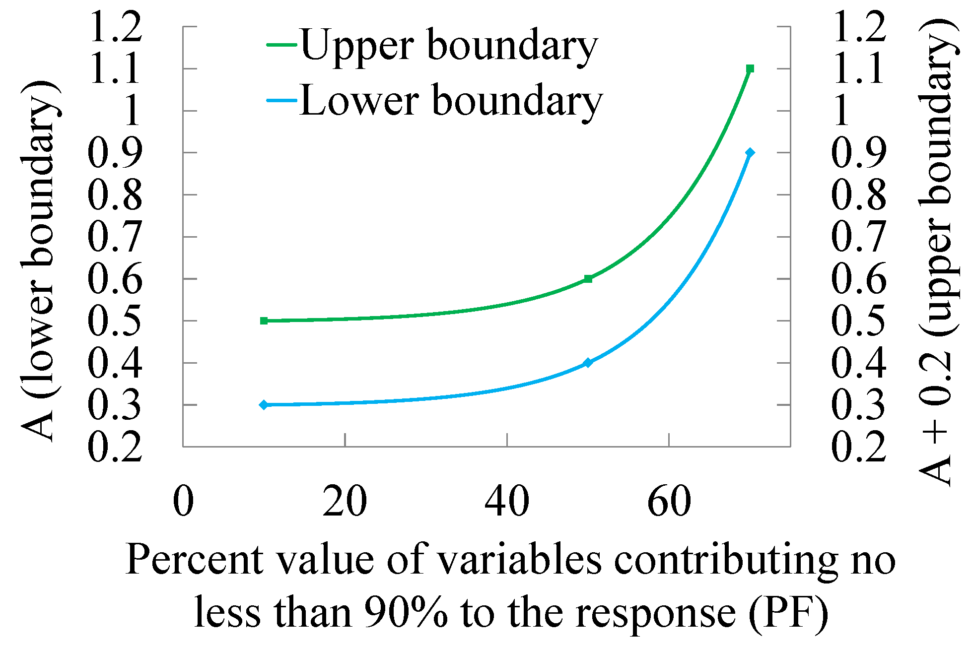
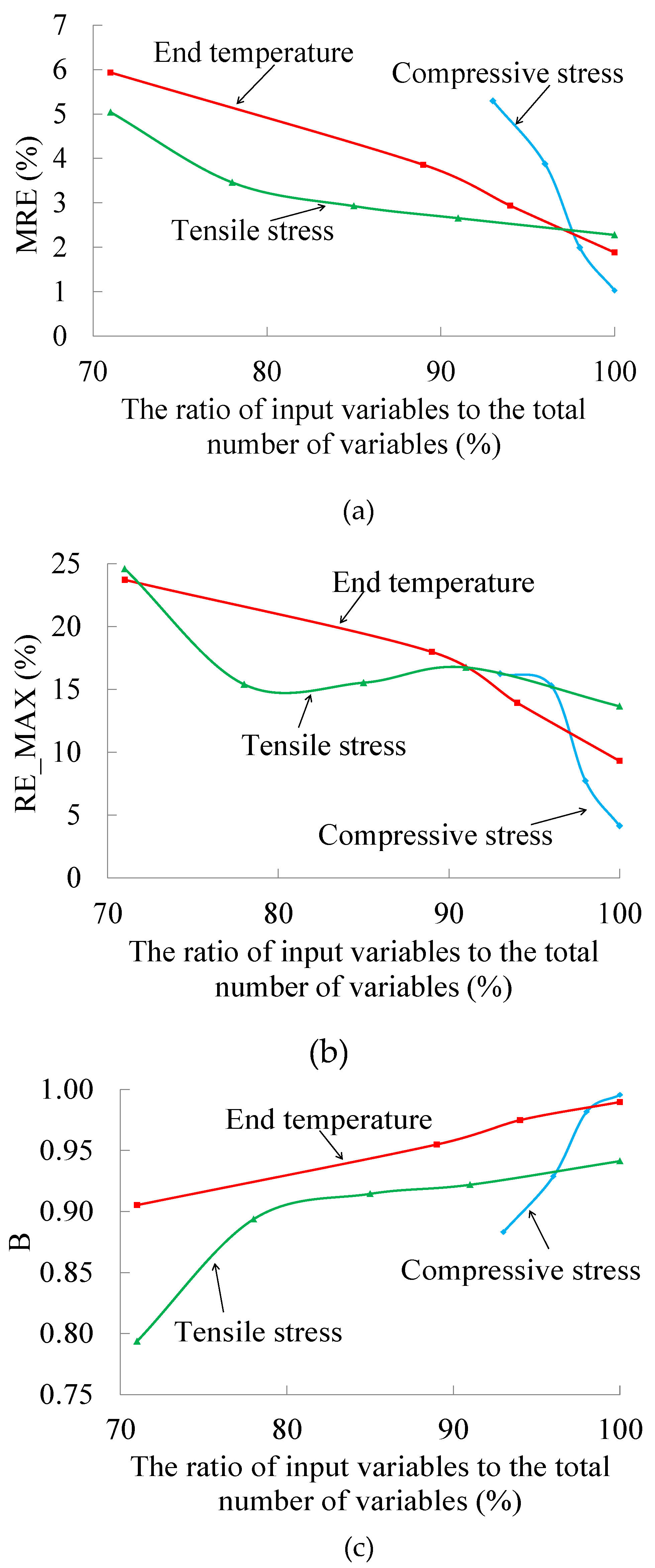
3.2. Influence of the Variable Completeness on the BP-ANN Prediction Performance

The combinations of input variables for each response are listed in Table 3. Each combination was fed as input to BP-ANN models with the node numbers in the hidden layer proposed in Table 4. For instance, the optimal node number in the hidden layer was 4, 5, and 6 for the maximum compressive stress. That is to say, three BP-ANN modeling were conducted for each input combination. The prediction performance was evaluated by the mean values of RE_MAX, MRE, and B of three BP-ANN models, shown in Figure 5. In general, for all three responses, lower RE_MAX and MRE and larger B can be achieved with increasing variable completeness. The minimum number of variables for each response was determined by an arbitrary chosen error tolerance, i.e., 15% of RE_MAX, 3% of MRE, and 0.90 of B and listed in

Table 7. Selection of the minimum number of input variables satisfying the predefined criteria.

Response	Minimum Number of Input Variables	Contribution to Response (%)
Compressive stress	3	98
End temperature	5	94
Tensile stress	6	85

with contribution summations of these variables to the response. The combinations consisted of the minimum number of variables that are capable of predicting the relation between input variables and corresponding outputs. It also indicates that the minimum number of variables changes with respect to the complexity of the problem. A larger number of variables shall be considered if the problem shows significant complexity, which shall contribute a certain value to the response. For instance, this value could be 90% for the tensile stress. This information further confirms the top priority of the significant factors of lining concepts analyzed with the Taguchi method.

4. Conclusions

The influence of variation/response space complexity and variable completeness on BP-ANN model establishment was investigated. The guidelines to define node numbers in the hidden layer were proposed for a steel ladle lining system according to the variation/response space complexity. The preferable node number ranges for maximum compressive stress at the hot face of the working lining, the end temperature, and the maximum tensile stress at the cold end of the steel shell were 4–6, 5–7, and 10–12, respectively. The minimum numbers of input variables of significance determined by the Taguchi method for the BP-ANN model were three, five, and six for the maximum compressive stress, the end temperature, and the maximum tensile stress.

The results evidently and exemplarily show that the variation/response complexity plays a determinant role in the architecture establishment of a BP-ANN model, which is often neglected in the applications of ANN models. The comparison study also demonstrates that the proposed guidelines in the present paper are efficient and can be extended into other fields in defining an optimal node number of the hidden layer in a three-layer BP-ANN model.

References

1. Flood, I. Towards the next generations of artificial neural networks for civil engineering. Adv. Eng. Inform. 2008, 22, 4–14. [Google Scholar] [CrossRef]
2. Mohandes, S.R.; Zhang, X.Q.; Mahdiyar, A. A comprehensive review on the application of artificial neural networks in building energy analysis. Neurocomputing 2019, 340, 55–75. [Google Scholar] [CrossRef]
3. Rodrigues, E.; Gomes, A.; Gaspar, A.R.; Antunes, G.H. Estimation of renewable energy and built environment-related variables using neural networks—A review. Renew. Sust. Energ. Rev. 2018, 94, 959–988. [Google Scholar] [CrossRef]
4. Ongpeng, J.M.C.; Oreta, A.W.C.; Hirose, S. Investigation on the sensitivity of ultrasonic test applied to reinforced concrete beams using neural network. Appl. Sci. 2018, 8, 405. [Google Scholar] [CrossRef]
5. Zhou, J.; Li, E.; Wei, H.; Li, C.; Qiao, Q.; Armaghani, D.J. Random forests and cubist algorithms for predicting shear strengths of rockfill materials. Appl. Sci. 2019, 9, 1621. [Google Scholar] [CrossRef]
6. Dobrzański, L.A.; Trzaska, J.; Dobrzańska-Danikiewicz, A.D. Use of neural network and artificial intelligence tools for modeling, characterization, and forecasting in material engineering. In Comprehensive Materials Processing; Hashmi, S., Batalha, G.F., Van Tyne, C.J., Yilbas, B., Eds.; Elsevier: Amsterdam, The Netherlands, 2014; Volume 2, pp. 161–198. [Google Scholar]
7. Park, T.C.; Kim, B.S.; Kim, T.Y.; Jin, I.B.; Yeo, Y.K. Comparative study of estimation methods of the endpoint temperature in basic oxygen furnace steelmaking process with selection of input parameters. Korean J. Met. Mater. 2018, 56, 813–821. [Google Scholar] [CrossRef]
8. Cox, I.J.; Lewis, R.W.; Ransing, R.S.; Laszczewski, H.; Berni, G. Application of neural network computing in basic oxygen steelmaking. J. Mater. Process. Technol. 2002, 120, 310–315. [Google Scholar] [CrossRef]
9. He, F.; Zhang, L. Prediction model of end-point phosphorus content in BOF steelmaking process based on PCA and BP neural network. J. Process Control 2018, 66, 51–58. [Google Scholar] [CrossRef]
10. Tunckaya, Y.; Koklukaya, E. Comparative performance evaluation of blast furnace flame temperature prediction using artificial intelligence and statistical methods. Turk. J. Electr. Eng. Comput. Sci. 2016, 24, 1163–1175. [Google Scholar] [CrossRef]
11. Strakowski, R.; Pacholski, K.; Wiecek, B.; Olbrycht, R.; Wittchen, W.; Borechi, M. Estimation of FeO content in the steel slag using infrared imaging and artificial neural network. Measurement 2018, 117, 380–389. [Google Scholar] [CrossRef]
12. Haykin, S. Neural Networks and Learning Machines; Pearson Education: Toronto, ON, Canada, 2009; p. 166. [Google Scholar]
13. Lopez, I.; Aragones, L.; Villacampa, Y.; Compan, P. Artificial neural network modeling of cross-shore profile on sand beaches: The coast of the province of Valencia (Spain). Mar. Georesour. Geotechnol. 2018, 36, 698–708. [Google Scholar] [CrossRef]
14. Bienvenido-Huertas, D.; Moyano, J.; Rodriguez-Jimenez, C.E.; Marin, D. Applying an artificial neural network to assess thermal transmittance in walls by means of the thermometric method. Appl. Energy 2019, 233, 1–14. [Google Scholar] [CrossRef]
15. Chen, D.; Singh, S.; Gao, L.; Garg, A.; Fan, Z. A coupled and interactive influence of operational parameters for optimizing power ouptut of cleaner energy production systems under uncertain conditions. Int. J. Energy Res. 2019, 43, 1294–1302. [Google Scholar] [CrossRef]
16. Darajeh, N.; Idris, A.; Masoumi, H.R.F.; Nourani, A.; Truong, P.; Rezania, S. Phytoremediation of palm oil mill secondary effluent (POMSE) by Chrysopogon zizanioides (L.) using artificial neural networks. Int. J. Phytoremediat. 2017, 19, 413–424. [Google Scholar] [CrossRef] [PubMed]
17. Darajeh, N.; Masoumi, H.R.F.; Kalantari, K.; Ahmad, M.B.; Shameli, K.; Basri, M.; Khandanlou, R. Optimization of process parameters for rapid absorption of Pb(II), Ni(II), Cu(II) by magnetic/talc nanocomposite using wavelet neural network. Res. Chem. Intermediat. 2016, 42, 1977–1987. [Google Scholar] [CrossRef]
18. Cao, Z.; Guo, N.; Li, M.H.; Yu, K.; Gao, K. Back propagation neural network based signal acquisition for Brillouin distributed optical fiber sensors. Opt. Express 2019, 27, 4549–4561. [Google Scholar] [CrossRef] [PubMed]
19. Luo, H.; Lai, F.; Dong, Z.; Xia, W. A lithology identification method for continental shale oil reservoir based on BP neural network. J. Geophys. Eng. 2018, 15, 895–908. [Google Scholar] [CrossRef] [Green Version]
20. Chokphoemphum, S.; Chokphoemphum, S. Moisture content prediction of paddy drying in a fluidized-bed drier with a vortex flow generator using an artificial neural network. Appl. Therm. Eng. 2018, 145, 630–636. [Google Scholar] [CrossRef]
21. Chen, X.; Xun, Y.; Li, W.; Zhang, J. Combining discriminant analysis and neural networks for corn variety identification. Comput. Electron. Agr. 2010, 71, 48–53. [Google Scholar] [CrossRef]
22. Onyari, E.K.; Ikotun, B.D. Prediciton of compressive and flexural strengths of a modified zeolite additive mortar using artificial neural network. Constr. Build. Mater. 2018, 187, 1232–1241. [Google Scholar] [CrossRef]
23. Amalia, A.; Suryono, S.; Suseno, J.E.; Kurniawati, R. Ultrasound-assisted extraction optimization of phenolic compounds from Psidium guagava L. using artificial neural network-genetic algorithm. In Proceedings of the 7th International Seminar on New Paradigm and Innovation on Natural Science and Its Application, Semarang, Indonesia, 17 October 2017. [Google Scholar] [CrossRef]
24. Heung, F.; Ching, T. The selection of pattern features for structural damage detection using an extended Bayesian ANN algorithm. Eng. Struct. 2008, 30, 2762–2770. [Google Scholar] [CrossRef] [Green Version]
25. Karsoliya, S. Approximating number of hidden layer neurons in multiple hidden layer BPNN architecture. IJETT 2012, 31, 714–717. [Google Scholar]
26. Hou, A.; Jin, S.; Harmuth, H.; Gruber, D. Thermal and thermomechanical responses prediction of a steel ladle using a back-propagation artificial neural network combing multiple orthogonal arrays. Steel Res. Int. 2019, 90. [Google Scholar] [CrossRef]
27. Hou, A.; Jin, S.; Harmuth, H.; Gruber, D. A method for steel ladle lining optimization applying thermomechanical modeling and Taguchi approaches. JOM 2018, 70, 2449–2456. [Google Scholar] [CrossRef]
28. MathWorks. Deep Learning Toolbox: User’s Guide; MathWorks: Natick, MA, USA, 2018. [Google Scholar]
Figure 1. Two-dimensional model representing steel ladle slag zone linings [26].
Applsci 09 02835 g001
Figure 2. A schematic of a three-layer artificial neural network (ANN) model.
Applsci 09 02835 g002
Figure 3. Performance assessment (a) RE_MAX—maximum relative error of all testing results, (b) MRE—mean relative error, and (c) B—coefficient of determination of the BP-ANN models with different node numbers in the hidden layer.
Applsci 09 02835 g003
Figure 4. The relation between PF and A (a function of PF).
Applsci 09 02835 g004
Figure 5. Performance assessment (a) RE_MAX, (b) MRE, and (c) B of BP-ANN models with different variable completeness (the ratio of input variables to the total number of variables).
Applsci 09 02835 g005