Estimating Maize-Leaf Coverage in Field Conditions by Applying a Machine Learning Algorithm to UAV Remote Sensing Images

Abstract

Leaf coverage is an indicator of plant growth rate and predicted yield, and thus it is crucial to plant-breeding research. Robust image segmentation of leaf coverage from remote-sensing images acquired by unmanned aerial vehicles (UAVs) in varying environments can be directly used for large-scale coverage estimation, and is a key component of high-throughput field phenotyping. We thus propose an image-segmentation method based on machine learning to extract relatively accurate coverage information from the orthophoto generated after preprocessing. The image analysis pipeline, including dataset augmenting, removing background, classifier training and noise reduction, generates a set of binary masks to obtain leaf coverage from the image. We compare the proposed method with three conventional methods (Hue-Saturation-Value, edge-detection-based algorithm, random forest) and a frontier deep-learning method called DeepLabv3+. The proposed method improves indicators such as Q_seg, S_r, E_s and mIOU by 15% to 30%. The experimental results show that this approach is less limited by radiation conditions, and that the protocol can easily be implemented for extensive sampling at low cost. As a result, with the proposed method, we recommend using red-green-blue (RGB)-based technology in addition to conventional equipment for acquiring the leaf coverage of agricultural crops.

1. Introduction

Plant phenotyping is an important tool for linking environmental and genetic research, and is used to evaluate drought and climate-change resistance by comparing the growth differences between plant varieties [1]. Plant researchers can bridge the gap between genomics and phenotype through field investigations [2]. Many types of phenotypic parameters available in the field are valuable for yield estimation and quality detection, such as plant height, spike number, leaf coverage, and so on. Among these, leaf coverage has a direct effect on the interception of photosynthetic radiation, water interception, heat fluxes, and CO₂ exchange. Leaf coverage can also be used as a key linkage between canopy reflectance and crop-growth models. Over the past decades, the study of leaf coverage evolved away from the general use of potted plants as research objects [3]. However, current methods, such as continuous imaging by fixed-position cameras, or destructive methods based on crop harvesting, are usually time-consuming.

Moreover, since crop growth can vary between outdoor and indoor environments, indoor observations are not suitable for predicting outdoor growth trends. Numerous adverse factors affect the precision of field phenotypic observations, such as differences in nutrients and water availability. Moreover, environmental influences such as wind, humidity, changing solar radiation, and cloud coverage also degrade data accuracy. To accurately and reliably study the in-field growth pattern of plant cultivars, researchers use high-throughput field phenotyping (HTFP), whereby phenotypic parameters are acquired by using automated or semi-automated systems. Currently, most HTFP-based systems for estimating leaf coverage use multispectral or hyperspectral images or RGB images. In the present study, we focus on the use of RGB images, because the associated technology is much lighter and cheaper than a spectral system, and can be fixed to a small unmanned aerial vehicle (UAV) platform. Digital photography is a popular tool for acquiring field information about small crops because it is affordable and easy to use with minimal training. The key step of extracting leaf coverage from RGB images is image segmentation, and existing segmentation methods for RGB images focus mainly upon two aspects: The first aspect is solely based on color information. For example, Dahan et al. presented a technique that synergistically combines depth and color image information from real devices. They use the color information to fill and clean depth and use depth to enhance color-image segmentation [4]. Panjwani and Healey introduced a segmentation method that uses a color Gaussian–Markov random-field model, which considers both spatial interactions within each spectral band and the interactions between color planes [5]. Shafarenko et al. explored a bottom-up segmentation approach that was developed to segment randomly-textured color images [6], and Hoang et al. put color and texture information together in the segmentation process to finish the segmentation of synthetic and natural images [7]. In addition, Xiong et al. introduced a segmentation method that combines the hue-saturation-value (HSV) color space and the Otsu method. Their experimental results show that the algorithm presented herein has a good effect and can meet real-time demand [8]. Thus, segmentation based on color information is seriously affected by the illumination. In this way, each type of method usually applies to a certain reproductive period. Except for the disadvantages described above, excess dependence on color information will lead to incomplete extraction. The second aspect of extracting leaf coverage from RGB images is based on the classifier. For example, Wang et al. introduced the novel fuzzy c-means approach (FCM), which uses local contextual information and the inherently high inter-pixel correlations to automatically segment images. Experimental results show that the proposed method provides competitive segmentation results compared with other FCM-based methods, and is generally faster [9]. Bai et al. presented an automated object-segmentation approach based on principal pixel analysis and a support vector machine, which effectively segments the entire salient object with reasonable performance and higher speed [10]. Recently, Chen et al. introduced a new segmentation method by combining three technologies: Deep Convolutional Nets, Atrous Convolution, and Fully Connected CRFs. This method is superior for dealing with complex conditions [11]. Moreover, Ravi et al. proposed a semantic segmentation of images by using multi-feature extraction and random forest (RF). According to their conclusion, this method offers good performance and accuracy in a small class [12]. Although all the methods mentioned above improve the processing accuracy of specific scenes in image processing, they still have many shortcomings. For example, the color-based segmentation methods are sensitive to changes in light intensity, and so they cannot be regarded as environmentally robust methods. 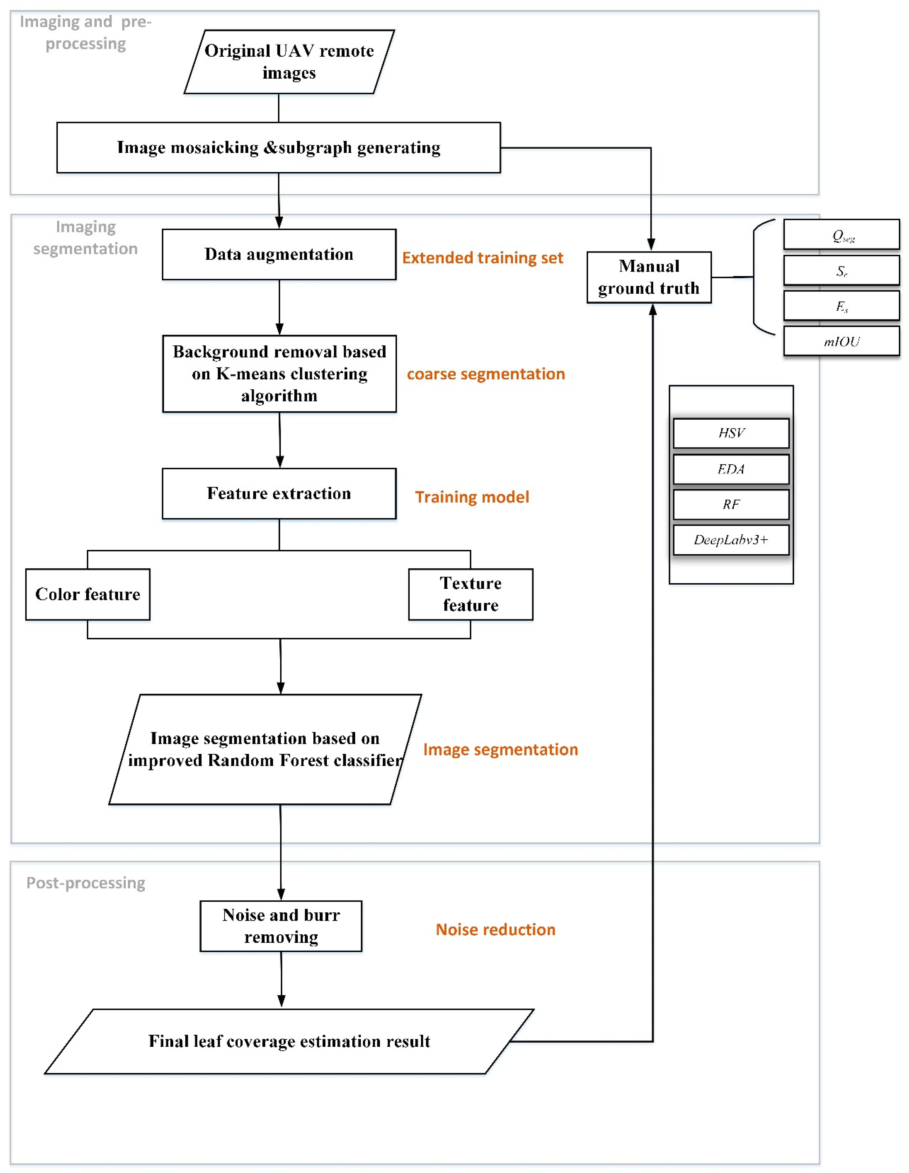Furthermore, deep-learning (DL) technology requires a large training set and high-performance hardware (e.g., a high graphics processing unit (GPU) frequency) [13]. To resolve these problems, we investigate herein a segmentation algorithm based upon an improved random forest classifier. First, the original UAV remote-sensing image dataset is augmented by three strategies, so that it can meet the requirement of big-data training. To highlight target characteristics, the background of the dataset is removed by using the K-means clustering algorithm. We then extract several image features, including color features and texture features, to describe the differences between the leaf part and the stem part. The improved RF classifier is trained by using the feature matrix and outputs the binary segmentation results.

Finally, 4 indicates including Q_seg, S_r, E_s, and mIOU are used to evaluate the segmentation accuracy by comparing the machine recognition results with the manual ground-truth reference images [14].

The rest of this paper is organized as follows: Section 2 briefly introduces the data acquisition and preprocessing, and Section 3 details the proposed algorithm. The experimental result and analysis are given in Section 4 and Section 5, respectively, and the conclusion is given in Section 6.

2. Data Acquisition and Preprocessing

This study covers 800 varieties of maize plants, and was conducted at the Xiaotangshan National Precision Agriculture Research and Demonstration Base (latitude 40°00′N–40°21′N, longitude 116°34′E–117°00′E, altitude 36 m) to study the genotype-by-environment interactions (Figure 1). In the present study, each variety was grown in a single plot to ensure independent growth. The sowing date was 12 May 2017 for the harvest year 2018, and the harvesting date was 5 September 2017.

2.1. Data Acquisition

This research uses images of seedling-stage maize plants for the segmentation dataset because of the low vegetation coverage and the ease of identifying the leaf boundary. With the further growth of maize, the images often contain 100% leaf coverage with no visible soil, which makes it difficult to separate the leaves from the background. To capture the canopy structure of the maize seedlings, a UAV-based image acquisition system was used to photograph the entire experimental area. This system consisted of two main parts: A flight mechanism (DJI-S1000, DJI Company, Shenzhen, China) and an RGB camera. The photos were taken from approximately 40 m above the canopy, looking vertically downward. A total of 83 photographs were obtained, with a lateral overlap of 50% and a longitudinal overlap of 70%. For this paper, we collected data in overcast and breezeless conditions to avoid shadows and target sloshing. The parameters of the digital camera used to acquire the images are given in

Table 1. Camera specifications.

Type	Manufacturer	Resolution	Pixel Size (μm2)	Ground Resolution (mm/pix)	Focal Length (mm)	FOV
QX-100	Sony	5472 × 3648	2.44 × 2.44	0.56	35	60°

. The color images were recorded in jpeg format and downloaded to desktop computers for subsequent processing.

2.2. Data Preprocessing

Segmenting plant leaves in the outdoors poses a unique challenge compared with the urban or interior environment commonly used for image segmentation [15]. Obtaining a strict leaf boundary is difficult because of the dynamic illumination conditions, leaf occlusion, and geometric variability between individual leaves [16]. In addition, the changing illumination conditions between images also increase the difficulty of segmentation.

2.2.1. Image Mosaicking and Generating Subgraphs

After obtaining 83 local images of the maize-breeding research field, all of the images were processed to obtain complete leaf-coverage information. Because of restrictions due to flight altitude and CCD size, most of the images acquired from the UAV remote-sensing platforms are image sequences with a small amplitude, low overlap and a large tilt angle. Furthermore, the RGB cameras carried on the UAV platforms contained mostly non-metric ordinary digital sensors, so the internal camera parameters are not known with precision. To solve these problems, we used the Photoscan Software (Agisoft, St. Petersburg, Russia) to preprocess the images as follows: (1) The selection of aerial photos, (2) image mosaicking, (3) generate digital elevation model (DEM) and orthophoto. We then used the Arcgis 10.2 to manually separate a single species from the orthophoto map according to the scope of the planting plot. Next, we used Photoshop (Adobe Inc., CA, USA) to generate several 1000 × 1000 pixel subgraphs in which the large-area ridges were removed.

2.2.2. Manual Ground Truth

We used Adobe Photoshop CS 6.0 to generate a segmentation mask for each plot; these masks were then used to manually annotate the boundary of each leaf in the image. To reduce any errors in the final masks, each image was treated three times by different workers to produce three unique masks, and the most accurate mask for each image was manually selected based on the overlay of the mask and the original image.

3. Methods

Leaf segmentation from a complex background requires selecting well-suited features and efficient segmentation methods, and the segmentation results must be verified so that the segmentation process may be corrected and refined if need be. Therefore, the image analysis pipeline includes four major steps: (1) Dataset augmentation, (2) background removal, (3) image segmentation, and (4) noise and burr removal (Figure 2).

3.1. Dataset Augmentation

Dataset augmentation is a common method to increase the size of a dataset and decrease overfitting during training [17]. Because the original image dataset is not large enough to satisfy the requirements for the training dataset, we divide the 800 images in our labeled dataset into 600 training and 200 validation image pairs, and then apply three techniques to augment the dataset: (1) mirror inverse, (2) 90° rotation, and (3) 180° rotation. These operations were all done by using Photoshop CS6, with the final result being a new final dataset with 2400 images for training and 800 for validation. To test the efficacy of this work, both the original and augmented datasets were used in parallel in our experiment.

3.2. Background Removal based on Improved K-means Clustering Algorithm

The background removal step serves to separate the vegetation from the soil. This is done by using the improved self-adaption K-means clustering algorithm. The principle of this algorithm is to minimize the sum of the squares of the distance from each point in the cluster domain to the center of the cluster [18]. This procedure consists of the following steps:

(a)

As initial clusters, choose k data points at random from the dataset.

(b)

Calculate the Euclidean distance from each data point x_i (i = 1,2,…,k) to each cluster center m_i and assign each data point to its nearest cluster center.

(c)

Calculate new cluster centers m_i so that the squared error distance of each cluster is a minimum.

(d)

Repeat steps (b) and (c) until the lustering centers m_i remain constant.

(e)

Terminate the process.

This method has two main disadvantages: First, the selection of these initial clustering centers may change the final clustering results, and second, it may cause the final result to become trapped in a local optimum. In this paper, we propose to solve these problems by using an improved K-means clustering algorithm based on Otsu multi-threshold segmentation. First, the Otsu algorithm was used for histogram multi-threshold segmentation, which divides each image into several classes and minimizes the variance between these classes. The improved algorithm is as follows:

(a)

Take the threshold of the Otsu segmentation T₁-T_k as the initial clustering center of the K-means algorithm.

(b)

Calculate the Euclidean distance from each data point x_i (i=1, 2, …, n) to each cluster center T_i and assign each data point to the nearest cluster center.

(c)

Calculate the new cluster center t_i to minimize the squared error distance of each cluster.

(d)

Repeat steps (b) and (c) until the clustering centers t_i remain constant.

(e)

Calculate the arithmetic mean for t_i and T_i and then obtain the final segmentation threshold M_i.

(f)

Use M_i to complete the image segmentation.

3.3. Leaf Exaction based on Multi-feature and Improved Random Forest Classifier

This study uses a machine-learning-based (ML-based) image segmentation method for leaf extraction, which transforms the image segmentation into a two-classification problem [19]. These techniques can be divided into two main learning groups; namely, supervised and unsupervised learning. The difference between the two types of methods is the pre-supply of information: Supervised techniques supply the information by pre-defined class labels or pre-trained samples, whereas unsupervised pattern representations do not require this operation [20]. In field conditions, variable light intensity and complex soil background make it crucial to extract crop-related characteristics. Based on this consideration, we develop a supervised multi-feature that is capable of training a model in different field conditions and labeling each image pixel as background or vegetation, regardless of the environmental conditions in the field.

3.3.1. Feature Extraction

Visual features are fundamental in processing digital images to represent image content. The result of feature extraction is that the points on the image are divided into different subsets, which often belong to isolated points, continuous curves, or continuous regions. In this paper, color, texture, and sharp features are extracted to discriminate between leaves and other parts. In this work, 6 color features and 16 texture features were used to describe each patch. In detail, feature definition and extraction involve the following items:

(1) Color features

Color feature is a global feature that describes the surface properties of objects. The colors green, brown, and yellow were found to compose the main part of the images of maize leaf collected in the field. Further analysis revealed that brown and yellow are common to vegetation and soil, whereas green is unique to vegetation. For this work, we extract six color components to describe the color distribution of each patch: R, G, B, L*, A*, B*.

(2) Texture features

Unlike color features, texture features are not based on single pixels, but must be extracted from regions. This regional aspect gives this approach strong fault tolerance because local deviation cannot cause matching failure.

A statistical aspect of texture features is that they are often rotation invariant, which makes them robust against noise. Crop images reveal different textures for leaf, stem, and soil. For example, leaf texture is clear because of the leaf stripe, whereas background texture is smooth because it is far from the camera. Here, we use the gray-level co-occurrence matrix (GLCM) to obtain the texture information from the images. The GLCM is defined as the joint probability distribution of pixel pairs, and not only reflects the comprehensive information from the adjacent direction and the adjacent interval, as well as the amplitude of change in the gray level of the image, but also reflects the spatial distribution of the pixels with the same gray level. We extract several texture features from the GLCM: The angular second moment, entropy, contrast, and correlation. The implications of these features are listed in

Table 2. Implication of texture features extracted from the gray-level co-occurrence matrix (GLCM). Types of features are angular second moment (ASM), entropy (ENT), contrast (CON), and correlation (COR).

Feature Kind	Computational Formula	Implication
ASM	$ASM={\displaystyle {\sum }_{i=1}^k{\displaystyle {\sum }_{j=1}^k{\left[G(i,j)\right]}^2}}$	Image gray distribution uniformity and textural detail
ENT	$ENT=-{\displaystyle {\sum }_{i=1}^k{\displaystyle {\sum }_{j=1}^{k}G(i,j)\log G(i,j)}}$	Image gray distribution heterogeneity or complexity
CON	$CON={\displaystyle {\sum }_{n=0}^{k-1}{n}^2\left[{\displaystyle {\sum }_{\left|i-j\right|=n}G(i,j)}\right]}$	Image clarity and texture depth
COR	$COR={\displaystyle {\sum }_{i=1}^k{\displaystyle {\sum }_{j=1}^k\frac{(ij)G(i,j)-u_i{u}_j}{s_i{s}_j}}}$	Local gray correlation in image

. We generate eight matrices in four directions (0°, 45°, 90°, 135°) with two lengths (1, 2) to extract eight features. In addition, the mean and variance of these four features for the two distances are treated as supplements of the texture feature, which makes a total of 16 features.

In Table 2, $G(i,j)$ is the element in row i and column j, and $u_i$, $u_j$,$s_i$, and $s_j$ are given by

$$u_i={\displaystyle \sum _{i=1}^k{\displaystyle \sum _{j=1}^{k}iG\left(i,j\right)}},$$

(1)

$$u_j={\displaystyle \sum _{i=1}^k{\displaystyle \sum _{j=1}^{k}jG\left(i,j\right)}},$$

(2)

$$s_i={\displaystyle \sum _{i=1}^k{\displaystyle \sum _{j=1}^{k}G(i,j)(i-u_i)}},$$

(3)

$$s_i={\displaystyle \sum _{i=1}^k{\displaystyle \sum _{j=1}^{k}G(i,j)(j-u_j)}}.$$

(4)

3.3.2. Proposed Image-Segmentation Model

By using the operations detailed above, image segmentation was transformed into building a two-class model. This model contains two types of samples: Positive samples (containing leaf patches manually labeled from different varieties) and negative samples (containing background patches manually labeled from soil and stem). We next built a training dataset with 24,000 positive patches (ten patches for each image) and 19,200 negative patches (eight patches for each image).

Each training patch contained 20 × 20 pixels to match the size of leaf, and the training patches were then represented in an M×N matrix called the “feature cube.” In this cube, M is the number of pixels in the patch (M = 400) whereas N is the number of features (N = 22 in the axis). To summarize, we built a training with enough positive and negative samples, which satisfies the requirements of the ML sample size.

We then used the improved random forest classifier to classify the model training based on the above dataset. The conventional random forest methods are an ensemble of learning methods for classification (and regression), that constructs a multitude of decision trees at training time and outputs the class that is the mode of the classes output by individual trees. It is a classifier composed of decision trees. By using $x\in X$ as sample data and $t\in T$ as an independent decision tree, the predictive function $h(x|t)$ can be expressed as

$$\left\{\begin{array}{c}\mathrm{nonleaf}\mathrm{node}:h(x|N(\psi ,t_l,t_r))=\left\{\begin{array}{l}h(x|t_l),\psi (x)=0\\ h(x|t_r),\psi (x)=1\end{array}\right\}\\ \mathrm{leaf}\mathrm{node}:h(x|L(\pi ))=\pi \end{array}\right\}$$

(5)

where $\psi (x)$ is the splitting function of each node in the decision tree, and π is the category information of a leaf. The voting model of a random forest F is

$$y^{*}=\underset{y\in Y}{\arg \max }{\displaystyle \sum _{t\in F}I\left(h(x|t)=y\right)},$$

(6)

where I is the indicator function, which can take on values in the range [0,1]. We define the function $f(x,{\theta }_i)$ as the i^th tree constructed by the random vector ${\theta }_i$. The random forest can then be represented by $F=\{f_1,f_2,\dots ,f_T\}$, where T is the scale of the forest. The margin function of the sample data (x, y) is

$$mg(x,y)=a{\nu }_{T}I\left(f_T(x)=y\right)-\underset{j\ne y}{\max }a{\nu }_{T}I\left(f_T(x)=j\right),$$

(7)

where $a{\nu }_T$ represents the average function. The generalization error can then be expressed as

$$GE=E_{(x,y)}\left(mg(x,y)<0\right).$$

(8)

In Equation (8), the subscripts x, y indicate that the probability runs over the x, y space. The generalization error GE has an upper bound that is defined as

$$GE*\le \overline{\rho }\frac{1-s^2}{s^2},$$

(9)

where $\overline{\rho }$ is the mean of the correlation and s is the strength of the set of classifiers. To reduce the correlation coefficient $\overline{\rho }$ of the decision trees, and widen the information field of the optional new feature attribute, we should improve the randomness when building the decision trees. The improved random forest algorithm is described in Algorithm 1. All decision trees in our experiment were constructed by using the CART tree, and the Gini index was used to measure purity of the node. In the following experiment, the number of the decision trees was set to 100 and then the best one of them was chosen to conduct repetitive experiments. The verification period is set to 1000 (i.e., the accuracy of the training model is tested 1000 times on the verification set per iteration of the network).

Algorithm 1

Input: initial training dataset as D, the number Fn of input features of each training sample.

Step 1: In a node of the decision tree to be split, $F=\lceil {\mathrm{rand}(0,\mathrm{F}}_N)\rceil$ attributes $(s_{1,}{s}_2,\dots s_F)$ are randomly selected from the set of sample attributes as the attributes to be combined. $\lceil •\rceil$ represents the rounding operation.

Step 2: Let $L=\lceil rand(0,\mathrm{int}(lb{F}_N+1))\rceil$ be weight vectors $(X_1,X_2,\dots X_L)$, where Xi is the vector of F times obtained from a real number sample in the interval (0, 1).

Step 3:L new features $(s{n}_1,s{n}_2,\dots ,s{n}_L)$ selected by the decision tree in the split node are obtained by linear weighted summation; that is, $s{n}_i=s_1*x_{il1}+s_2*x_{il2}+\cdots +s_F*x_{ilF};i=1:L$.

Step 4: The best new feature is selected by the Gini index as the splitting property of the node. The Gini index can be used to measure the purity of the node, and we use the minimum distance based on the Gini index to select the splitting attribute.

Step 5: Each node is constructed recursively until the node sample has only a single category, which guarantees the complete growth of the decision tree.

Step 6: Repeat steps (1)–(5) N times to generate a random forest of scale N.

The improved random forest algorithm proposed herein further extends the attribute domain, which further reduces the relativity of the decision tree. Since the improved RF does not restrict the amount of the combining features, the mean value of the linear combination feature number is a random one. Thus, the original feature space F can be expanded to a $\gamma$-dimensional $(\gamma =C_N^1+C_N^2+\cdots +C_N^N)$ feature space that contains not only the original feature space, but also any combination of features. C here represents a combination of features. Compared with the traditional random forest algorithm, the feature information space of the proposed algorithm is more extensive.

3.4. Noise and Burr Removal

After finishing the image segmentation, some noise points or burrs remained. To remove these sources of noise, and thereby improve the accuracy of the segmentation result, we used a median filter w to minimize the noise, and then removed the result of the burrs and the noise from the binary image. A three-pixel window was slid over the entire image, pixel by pixel, and the pixel values from the window were sorted numerically and replaced with the median of the neighboring pixels.

3.5. Evaluation Methods

The accuracy of the segmentation was then evaluated with three quality factors: Q_seg, S_r, and an error factor E_s. The factor Q_seg is based on both kernels and background regions, and ranges from zero to unity. Q_seg reflects the consistency of all the image pixels, including the leaf part and the remaining part, and Q_seg = 1 represents a perfect outcome. Conversely, the factor S_r reflects the consistency of only the leaf parts. From the perspective of an image, it reflects the completeness of the segmentation results. Furthermore, E_s indicates the portion of misclassified leaf pixels relative to true total leaf pixels. These evaluation indicators are calculated as follows:

$$Q_{seg}=\frac{{\displaystyle \sum \begin{array}{c}i,j=a,b\\ i,j=0\end{array}\left[M{(\delta )}_{i,j}\cap {N(\delta )}_{i,j}\right]}}{{\displaystyle \sum \begin{array}{c}i,j=a,b\\ i,j=0\end{array}\left[M{(\delta )}_{i,j}\cup {N(\delta )}_{i,j}\right]}},$$

(10)

$$S_r=\frac{{\displaystyle \sum \begin{array}{c}i,j=a,b\\ i,j=0\end{array}\left[M{(\delta )}_{i,j}\cap {N(\delta )}_{i,j}\right]}}{{\displaystyle \sum \begin{array}{c}i,j=a,b\\ i,j=0\end{array}\left[{N(\delta )}_{i,j}\right]}},$$

(11)

$$E_s=\frac{{\displaystyle \sum \begin{array}{c}i,j=a,b\\ i,j=0\end{array}\left[M{(\delta )}_{i,j}\cap {N(!\delta )}_{i,j}\right]}}{{\displaystyle \sum \begin{array}{c}i,j=a,b\\ i,j=0\end{array}\left[{N(\delta )}_{i,j}\right]}},$$

(12)

where M is the set of leaf pixels ($\delta$ = 1) or pixels for other parts ($\delta$ = 0) separated by the segmentation method, N is the ground truth for these two parts, i, j are the row and column coordinates of an image, respectively, and a, b are the width and height of the image, respectively. Furthermore, “$\cap$” is a logical “and”, “$\cup$” is a logical “or”, and “!” is a logical “not”. The accuracy of the segmentation can be measured by comparing M and N on a pixel-by-pixel basis. In addition, the mean intersection-over-union (mIOU) serves to determine the processing precision for the validation sets. It generates two boxes called the “predicted bounding box” and the “ground-truth bounding box,” and then compares the overlap rate between them. The schematic diagram and formula are given by

$$mIOU=\mathrm{mean}\left(\frac{\mathrm{Detection}\mathrm{Leaf}\mathrm{Area}\cap \mathrm{Ground}\mathrm{Truth}}{\mathrm{Detection}\mathrm{Leaf}\mathrm{Area}\cup \mathrm{Ground}\mathrm{Truth}}\right).$$

(13)

Our goal is to take the training images plus the bounding boxes, construct an object detector, and then evaluate its performance on the testing set. The mIOU varies within the range [0, 1], and mIOU > 0.5 is normally considered a “good” prediction.

4. Results

This section compares the performance of the RF-based image segmentation method with the performance of three other conventional segmentation methods: HSV segmentation based on color thresholding, edge detection-based image segmentation, and the convolutional neural network model called “DeepLabv3+” (

Table 3. Parameter settings of DeepLabv3+.

output_stride	16
crop_size	513 × 513
initial_learning rate	0.007
atrous rates	[6,12,18]

). Moreover, the traditional RF method is also introduced to compare with the improved RF algorithm proposed herein. The HSV color space differs from the standard RGB color space, because the former separates the pixel intensity from the actual color of the image. This is useful for our dataset because illumination conditions varied between images due to outdoor conditions. Using only the hue channel from the HSV image, we applied an Otsu threshold to extract the leaf area from the other parts of the image. The edge-detection-based algorithm (EDA) completes the image segmentation by detecting the gray-level mutation part. This type of mutation generally corresponds to an extreme point of the first-order derivative, or the zero crossing of the two derivatives. In this paper, we use the Roberts operator as a differential operator for our edge detection. Furthermore, DeepLabv3+ is a convolutional neural network model designed for pixel-based semantic image segmentation. It builds upon the DeepLabv3 design and combines a spatial pyramid pooling structure with an encoder-decoder structure, in order to achieve state-of-the-art segmentation results. Note that the DeepLabv3+ is based on the open source code available at https://github.com/tensorflow/models/tree/master/research/deeplab. The checkpoint was initialized by using the PASCAL VOC dataset with the following parameters. We also used the following hyper-parameters in all our experiments: The Base Learning Rate was 0.01, the Momentum was 0.9, the Dropout was 0.5, and the Iteration Time was 1000.

4.1. Estimating Maize Leaf Coverage with Different Image-segmentation Methods

To validate the use of the segmentation model with different theoretical bases, including color space transformation (HSV), gray-level-change detection (edge detection), ML (RF and improved RF), and DL (DeepLabv3+), all images in the dataset (i.e., the 600 original images and the 1800 augmented images) were used to train the model. Here, to show the reliability of the different methods, we choose five sample subgraphs with different leaf coverage (Figure 3).

4.2. Segmentation Accuracy

Figure 4 compares the accuracy of the segmentation (Q_seg, S_r, E_s) of the proposed method with that of four other methods. The HSV and EDA produce a relatively low Q_seg with the highest standard deviation (SD). Furthermore, DeepLabv3+ and RF are second and third, with an average Q_seg of 0.65 and 0.82 and a much lower SD. Of all these methods, the improved RF method produces the highest mean value of Q_seg and has the lowest SD. It also produces the highest S_r and the lowest SD. For the E_s index, HSV produces the most misclassified pixels, and the improved RF method produces the fewest misclassified pixels.

To test the efficacy of the augmentation, the image dataset without the augmented images was used independently.

From the results given in

Table 4. mIOU scores for different methods applied to the training or validation dataset.

Method	mIOU
HSV	0.4728
EDA	0.5941
RF	0.7316
DeepLabv3+	0.7984
Improved RF	0.8237

and

Table 5. mIOU scores for different methods applied to the original training and validation datasets.

Method	mIOU	Change (%)
HSV	0.4021	17.5
EDA	0.5364	10.8
RF	0.6897	6.1
DeepLabv3+	0.7916	0.9
Improved RF	0.8055	2.3

, we conclude that two classifier-based segmentation methods (DeepLabv3+ and the improved RF) produce the highest mIOU scores (0.7984, 0.8237 and 0.7916, 0.8055, respectively) which indicates that these two methods perform well on alternative datasets. These two methods also produce the smallest change in the mIOU score for the two training sets (0.9% and 2.3%), which means that they maintain good segmentation even when the quantity of data changes. The mIOU score in Table 5 is better than that in Table 4 because the augmentation of the original dataset improves the final accuracy.

The introduced techniques were also compared with the three well-known color index methods, the excess green index (ExG), the excess green minus ExGR and the color index of vegetation extraction (CIVE) [21]. We used ExG to provide a clear contrast between kernels and background: ExG = 2 × Green − Red − Blue. It used an automatic thresholding method that enabled background and foreground segmentation based on the bimodal distribution of the pixel. ExGR combined ExG and the excess red index to improve the performance of ExG: ExGR = ExG − (1.4 × R − G). CIVE evaluated color features by providing a greater emphasis on the green area: CIVE = 0.441R − 0.811G + 0.385B + 18.78745.

We concluded from the results in

Table 6. Comparison of segmentation quality for ExG, ExGR, CIVE and the proposed method (improved RF).

Method	Qseg	Sr	Es	mIOU
ExG	0.59	0.57	0.45	0.38
ExGR	0.61	0.60	0.38	0.47
CIVE	0.55	0.53	0.46	0.50
Improved RF	0.87	0.86	0.18	0.81

that relative to the other three common methods mentioned in this paper, the proposed method could obtain a greater mean value of these four indicators. It produced the highest quality of segmentation indices among the other three algorithms and had the lowest misclassification rate.

5. Discussion

The goal of this study is to find a reliable way to estimate the leaf coverage in the maize seedling stage based on UAV remote-sensing images. To reduce cost and improve efficiency, this goal is achieved by using image-processing technology rather than labor-intensive field surveys. To be able to use this efficient image-based method in all conditions, it must be sufficiently robust to handle dynamic illumination conditions and complex changes in morphology. Thus, to produce robust results, the image analysis pipeline must consider the various perturbing effects. Verifying the accuracy of these segmentation methods can also be a significant challenge. Although the experimental results in Section 4 for the proposed improved RF-based method are consistent with the manual validation data, further research is required to determine the adaptability of the proposed method. The results show that the segmentation accuracy depends strongly on the light intensity, the resolution of the training image and the sensitivity to noise. Here, we analyze how these factors affect the accuracy of the segmentation results.

5.1. Dependence of Image-segmentation Models on Illumination

In the field, the light intensity changes constantly. Unlike single plants grown in pots in greenhouse facilities, segmenting vegetation in a field-grown plot is complex. Factors such as changing weather conditions, and the solar radiation angle that evolves during the day, affect the results of the image segmentation.

To study how the method responds to different illumination conditions, we used the image brightness function of Photoshop CS6 to adjust the luminance components. The original image brightness was used as the central value for the brightness adjustment, to produce five images of varying luminance (two brighter and two darker than the central value).

The color lines in Figure 5 show how the indices vary as a function of the illumination conditions when using the proposed improved RF method and the four comparison methods. Specifically, almost all these methods have the lowest Q_seg and the highest E_s for Level 1 light intensity, which indicates that low illumination intensity seriously degrades the image-segmentation accuracy. The improved RF method and DeepLabv3+ method produce the highest Q_seg and S_r for Level 2 light intensity, whereas the three other methods do the same for Level 3, which indicates that the moderate light intensity tends to improve the image-segmentation accuracy. Furthermore, the improved RF and DeepLabv3+ methods performed well for all evaluation indicators (with larger values and smaller SD), indicating that they are less sensitive to varying illumination intensity. The accuracy should be further improved by expanding the training dataset, introducing more pixel-based features, and in particular, by adding images under different illumination conditions for training.

5.2. Dependence of Image-segmentation Models on Image Resolution

Choosing original images with the proper resolution is vital for ensuring operational efficiency and accuracy. We therefore verified the reliability of the proposed method for various image resolutions. The lower-resolution images were resized to four different resolutions by scaling down the original image resolution to obtain images with resolutions ranging from 1024 × 1024 pixels to 32 × 32 pixels.

Figure 6 shows the segmentation accuracy for different image resolutions. The curve shows that the resolution of the input image strongly affects the image-segmentation accuracy for both the HSV and EDA methods, which we attribute to their pixel-based characteristics. The color characteristics, or the grey level, change completely when the image resolution changes. No such abnormal fluctuation appears in the results of the other three ML-based or DL-based methods, because their accuracy depends only on the size of the training set, and not on the resolution of the input images. Thus, cameras with lower resolution, such as GoPro or mobile phone cameras, could be adapted to furnish the data.

5.3. Dependence of Image-segmentation Models on Image Noise

Image degradation caused by random errors is called image noise. Generally speaking, all factors that hinder the human perception of images can be called “noise”. The process of image generation often introduces noise that degrades the images. Image noise can be divided into two general categories: External noise and internal noise. External noise refers to noise caused by sources external to the system, whereas the internal noise refers to noise caused by the internal electronics of the system. To determine whether noise degrades the image-segmentation accuracy, we generated noisy versions of the original dataset and of the augmented dataset by adding three types of noise: Gaussian, Poisson, and salt and pepper noise. In addition, to understand how the use of a denoising algorithm for preprocessing affects the final results, we filtered the noisy data through a denoising median filter.

As shown in Figure 7, the results of the improved RF method with no noise filter are more accurate than those for the HSV, EDA, and RF methods, but slightly less accurate than the results of the DeepLabv3+ method.

However, when using the median filter, the results of the improved RF method are more accurate than those of the DeepLabv3+ method, which shows that noise reduction is important for proper feature extraction.

6. Conclusions

Timely extraction of meaningful data from a large number of high-resolution images is currently the bottleneck in high-throughput field phenotyping, so developing more rapid image-analysis pipelines is imperative. In the present study, we use an improved RF-based segmentation method to estimate maize leaf coverage in the seedling stage. First, a custom training and validation image dataset captured by using a UAV remote-sensing platform was preprocessed through a standardization procedure. Features based on color and texture were then input into an improved RF classifier as the training target, which we used to generate a set of binary masks for leaf coverage in the images. A comparison with four conventional color-based or DL-based methods shows that the proposed method produces more accurate image-segmentation results (an improvement of 15%–30%) as per the established evaluation system. Two main conclusions are warranted, based on these experimental results: (i) The dataset size is critical for DL methods, and (ii) preprocessing the data to ensure the correct color space improves the results for all methods. Based on the characteristics of ML itself, more abundant training data are crucial to improving the accuracy of the results. In future research, the use of an alternative augmentation method would be the easiest to test without requiring more data collection. In addition, we should add multiple precomputed features to the input data in order to increase the performance of the model.

References

1. Fiorani, F.; Schurr, U. Future Scenarios for Plant Phenotyping. Annu. Rev. Plant Biol. 2013, 64, 267–291. [Google Scholar] [CrossRef] [PubMed] [Green Version]
2. Lupski, J.R.; Stankiewicz, P. Genomic disorders: Molecular mechanisms for rearrangements and conveyed phenotypes. PLoS Genet. 2005, 1, e49. [Google Scholar] [CrossRef] [PubMed]
3. Singh, D.; Singh, K.P.; Sharan, S.K. Microwave response to broad leaf vegetation (Spinach) and vegetation covered moist soil for remote sensing. J. Indian Soc. Remote Sens. 2000, 28, 153–158. [Google Scholar] [CrossRef]
4. Dahan, M.J.; Chen, N.; Shamir, A.; Cohen-Or, D. Combining color and depth for enhanced image segmentation and retargeting. Vis. Comput. 2012, 28, 1181–1193. [Google Scholar] [CrossRef]
5. Panjwani, D.K.; Healey, G. Unsupervised segmentation of textured color images using Markov random field models. In Proceedings of the IEEE Computer Society Conference on Computer Vision & Pattern Recognition (CVPR), New York, NY, USA, 15-17 June 1993. [Google Scholar]
6. Shafarenko, L.; Petrou, M.; Kittler, J. Automatic watershed segmentation of randomly textured color images. IEEE Trans. Image Process. 1997, 6, 1530–1544. [Google Scholar] [CrossRef] [PubMed]
7. Hoang, M.A.; Geusebroek, J.M.; Smeulders, A.W.M. Color texture measurement and segmentation. Signal Process. 2005, 85, 265–275. [Google Scholar] [CrossRef]
8. Xiong, L.L.; Wang, X.Z. Research of Double-Threshold Segmentation of Brazing-Area Defect of Saw Based on Otsu and HSV Color Space. In Proceedings of the International Congress on Image & Signal Processing, Tianjin, China, 17–19 October 2009. [Google Scholar]
9. Wang, W.; Zhang, Y.; Yi, L.; Zhang, X. The Global Fuzzy C-Means Clustering Algorithm. In Proceedings of the World Congress on Intelligent Control & Automation, Dalian, China, 21–23 June 2006. [Google Scholar]
10. Bai, X.; Wang, W. Principal pixel analysis and SVM for automatic image segmentation. Neural Comput. Appl. 2016, 27, 45–58. [Google Scholar] [CrossRef]
11. Chen, L.C.; Papandreou, G.; Kokkinos, I.; Murphy, K.; Yuille, A.L. Semantic Image Segmentation with Deep Convolutional Nets and Fully Connected CRFs. IEEE Trans. Pattern Analysis & Machine Intelligence. 2014, 4, 357–361. [Google Scholar]
12. Ravì, D.; Bober, M.; Farinella, G.M.; Guarnera, M.; Battiato, S. Semantic segmentation of images exploiting DCT based features and random forest. Pattern Recognit. 2016, 52(C), 260–273. [Google Scholar] [CrossRef]
13. Valindria, V.V.; Lavdas, I.; Bai, W.; Kamnitsas, K.; Aboagye, E.O.; Rockall, A.G.; Glocker, B. Reverse Classification Accuracy: Predicting Segmentation Performance in the Absence of Ground Truth. IEEE Trans. Med. Imaging 2017, 36, 1597–1606. [Google Scholar] [CrossRef] [PubMed] [Green Version]
14. Zhang, S.; You, Z.; Wu, X. Plant disease leaf image segmentation based on superpixel clustering and EM algorithm. Neural Comput. Appl. 2019, 31, 1225–1233. [Google Scholar] [CrossRef]
15. Bakhshipour, A.; Jafari, A.; Nassiri, S.M.; Zare, D. Weed segmentation using texture features extracted from wavelet sub-images. Biosyst. Eng. 2017, 157, 1–12. [Google Scholar] [CrossRef]
16. Han, D.; Liu, Q.; Fan, W. A new image classification method using CNN transfer learning and web data augmentation. Expert Syst. Appl. 2018, 95, 43–56. [Google Scholar] [CrossRef]
17. Leng, B.; Kai, Y.; Yu, L.; Qin, J. Data Augmentation for Unbalanced Face Recognition Training Sets. Neurocomputing 2017, 235, 10–14. [Google Scholar] [CrossRef]
18. Zhao, F.; Chen, Y.; Hou, Y.; He, X. Segmentation of blood vessels using rule-based and machine-learning-based methods: A review. Multimed. Syst. 2017, 4, 1–10. [Google Scholar] [CrossRef]
19. Yang, B.; Ma, A.J.; Yuen, P.C. Learning Domain-Shared Group-Sparse Representation for Unsupervised Domain Adaptation. Pattern Recognit. 2018, 81, 615–632, S0031320318301614. [Google Scholar] [CrossRef]
20. Cai, Q.; Liu, H.; Zhou, S.; Sun, J.; Li, J. An adaptive-scale active contour model for inhomogeneous image segmentation and bias field estimation. Pattern Recognit. 2018, 82, 79–93, S0031320318301729. [Google Scholar] [CrossRef]
21. Hamuda, E.; Glavin, M.; Jones, E. A survey of image processing techniques for plant extraction and segmentation in the field. Comput. Electron. Agric. 2016, 125, 184–199. [Google Scholar] [CrossRef]
Figure 1. Description of the study area and design of the data acquisition based on an unmanned aerial vehicle (UAV) platform. (A) Schematic diagram of experimental area and selected plots, (B) Location of sampling points and ground control points.
Applsci 09 02389 g001
Figure 2. Workflow of a semi-automated method used to estimate leaf coverage.
Applsci 09 02389 g002
Figure 3. Estimate of the maize leaf coverage generated by different methods. Panels (ae) show leaf-coverage images selected at random from the dataset.
Applsci 09 02389 g003
Figure 4. Comparison of the mean accuracy rate (Qseg, Sr, and Es). Comparison of the segmentation quality for the hue-saturation-value (HSV), edge-detection-based algorithm (EDA), random forest (RF), DeepLabv3+, and the proposed method (improved RF). The color bars indicate the mean value of the indices, and the black lines represent their standard deviations.
Applsci 09 02389 g004
Figure 5. Results of image segmentation models for different illumination conditions. The color lines in each box represent how the indexes vary as illumination conditions when using different methods. Panels 1–5 show the results for light intensities ranging from dark to bright.
Applsci 09 02389 g005
Figure 6. Results of image segmentation models for different image resolutions. The color lines in each box represent how the indices vary as image resolution when using different methods. Panels 1–5 correspond to image resolution ranging from high to low.
Applsci 09 02389 g006
Figure 7. Results of image-segmentation methods for input data with different noise added. The color points in each box represent how the indices vary as different types of noise are added. Panels 1–6 show the results for the different types of noise: (1) Gaussian, (2) Poisson, (3) salt and pepper, (4) Gaussian noise removed by a median filter, (5) Poisson noise removed by a median filter, (6) salt and pepper noise removed by a median filter.
Applsci 09 02389 g007