Hybrid Artificial Intelligence Approaches for Predicting Critical Buckling Load of Structural Members under Compression Considering the Influence of Initial Geometric Imperfections

Abstract

The main aim of this study is to develop different hybrid artificial intelligence (AI) approaches, such as an adaptive neuro-fuzzy inference system (ANFIS) and two ANFISs optimized by metaheuristic techniques, namely simulated annealing (SA) and biogeography-based optimization (BBO) for predicting the critical buckling load of structural members under compression, taking into account the influence of initial geometric imperfections. With this aim, the existing results of compression tests on steel columns were collected and used as a dataset. Eleven input parameters, representing the slenderness ratios and initial geometric imperfections, were considered. The predicted target was the critical buckling load of columns. Statistical criteria, namely the correlation coefficient (R), the root mean squared error (RMSE), and the mean absolute error (MAE) were used to evaluate and validate the three proposed AI models. The results showed that SA and BBO were able to improve the prediction performance of the original ANFIS. Excellent results using the BBO optimization technique were achieved (i.e., an increase in R by 7.15%, RMSE by 40.48%, and MAE by 38.45%), and those using the SA technique were not much different (i.e., an increase in R by 5.03%, RMSE by 26.68%, and MAE by 20.40%). Finally, sensitivity analysis was performed, and the most important imperfections affecting column buckling capacity was found to be the initial in-plane loading eccentricity at the top and bottom ends of the columns. The methodology and the developed AI models herein could pave the way to establishing an advanced approach to forecasting damages of columns under compression.

1. Introduction

Initial imperfections of structural members could be classified into three main categories: geometric imperfections, fluctuations in mechanical properties of material, and residual stresses [1]. These imperfections directly result from manufacturing processes [2] or after the assembly of parts [3]. As reported in many experimental studies, imperfections are crucial for structural elements regarding their initial design, especially for those under compression [4,5,6]. For instance, in the work of Shi et al. [7], the authors demonstrated the existence of initial out-of-straightness imperfections of hollow circular tubes under axial loading by measuring the mid-length deflection over 24 specimens. The loading eccentricity was also measured by applying compression forces to pinned–pinned columns. As a result, the ratios of initial geometric imperfections to effective length varied from 0.15 to 12.12%, which led to a reduction of buckling capacity from 10 to 20% compared with the initial design. It was noticed that the yield strength, ultimate tensile stress, and elastic modulus fluctuations also existed in circular steel tubes [3,7]. These defects have a great influence on mechanical behaviors, causing a decrease in the buckling capacity of tubes under axial loading [3,7]. In addition, many experimental studies have shown that buckling appeared earlier than estimated because of initial imperfections, such as in the case of I-sections [6,8], box sections [3,9,10], equal angle columns [11,12,13], T-sections [14], circular sections [15,16], and C-sections [17,18,19] for steel structures or concrete structures [20,21,22], composite structures [23,24,25], and alloy structures [26,27,28,29].

Miscellaneous works on modeling and simulation have accounted for the initial imperfections of structural elements under axial compression in the literature. Analytical approaches based on high order shear deformation theory to take into account initial geometric imperfections have been reported for cylinder shells [30], annular spherical segments [31], or plates [32]. Nevertheless, analytical solutions often demonstrate a limitation as the structures are simplified with regular geometry. In the case of more complex structures, the numerical finite element technique has been widely applied to investigate the influence of initial imperfections on the buckling behavior of compression members, such as sigma section members [17], I-section steel columns wrapped by carbon fibers [24], cylindrical pipes made by carbon fiber-reinforced plastic material [23], braced columns [33], and multi-layer beams [25]. However, finite element analysis of buckling problems is mainly based on commercial software, for instance, ANSYS [7,19], ABAQUS [23,27], and NASTRAN [17]. Such typical instability problems exhibit a highly nonlinear relationship between load and displacement (i.e., small load increments induce large deformations) [6,8]. For that reason, finite element code implementing iterative techniques (e.g., the arc-length method [34], the Newton–Raphson technique [35], or normal flow [36]) to capture the nonlinear behavior of compression members remains a challenge for researchers. In addition, the use of commercial finite element software exposes several inconveniences such as choosing robust elements [27], mesh size convergence [37], and especially the generation of a large dataset integrating various types of initial imperfections [38,39,40,41].

Over the last two decades, a new and robust branch of computational mechanics using artificial intelligence (AI) approaches has been widely applied, especially for predicting the failure of structural members [42,43,44,45,46,47]. As an example, Jimenez-Martinez et al. [48] introduced an artificial neural network (ANN) algorithm for investigating the fatigue problem of chassis components. In addition, the durability of structural components subjected to cyclic loading was evaluated using a neural network in the work of Didych et al. [49], whereas the failure of concrete columns under fire using a data-driven technique was reported by McKinney et al. [50]. The investigation on instability of columns under axial compression using an AI-based approach was promising but still limited, particularly for accounting initial imperfections of structural elements. The ANN models have been introduced in several studies for predicting critical buckling load, such as in the work of Kumar et al. [51] on beam-columns, in the studies of Tahir et al. [52] on thin cylindrical shells, in work by Hasanzadehshooiili et al. [53] on arch-shells, and in work by Mallela et al. [54] for laminated panels. Last but not least, Bilgehan et al. [55] developed an adaptive neuro-fuzzy inference system (ANFIS) to estimate the column buckling load that takes into account initial cracks. Above all, several remaining issues need to be clarified: (i) the parameter optimization of AI methods, (ii) the possibility of treating the problem with other AI algorithms, especially the use of hybrid models, and (iii) sensitivity analysis of factors that affect the buckling responses of structural members under compression.

Therefore, the main objective of this work is to develop hybrid AI approaches involving ANFIS, ANFIS optimized with simulated annealing (SA), and ANFIS optimized with biogeography-based optimization (BBO) for predicting critical buckling load, or the maximum load capacity, of compression members, taking into account local, flexural-torsional, flexural failure modes and initial geometric imperfections. The SA and BBO optimization techniques were implemented to increase the prediction performance of the initial ANFIS model. The developed hybrid AI models were constructed and performed with data available in the literature on the buckling behavior of Y-section steel columns. Input parameters of the models were divided into two main groups—slenderness ratios (including 2 inputs) and initial geometric imperfections (with 9 inputs), respectively—while the output was the critical buckling load of the columns. Statistical criteria, namely the correlation coefficient (R), the root mean squared error (RMSE), and the mean absolute error (MAE), were evaluated at the end of the numerical simulations in order to investigate the prediction capability and performance of the AI models. Sensitivity analysis was finally performed with the aim of estimating the influence of input parameters on the predicted results, particularly focused on the initial imperfections.

2. Research Significance

As reported in the introduction, the determination of the critical buckling load of columns is important in the fields of mechanics and civil engineering applications. As instability is a complex non-linear problem, which depends on various parameters, the estimation of the buckling capacity has been challenging for researchers/engineers. Although miscellaneous experimental studies have addressed this problem, it is difficult to deduce a generalized formulation, taking into account all the parameters that affect the buckling behavior of columns. The use of soft computing techniques could help to explore the nonlinear relationships between the desired targets and the inputs of the problem, especially the initial geometric imperfections. The as-obtained information could help researchers/engineers quickly assess buckling resistance and reduce costly and time-consuming laboratory experiments. The sensitivity analysis using the developed AI models could also provide useful instructions that might be used to increase the compression capacity of columns.

3. Materials and Methods

3.1. Machine Learning Methods

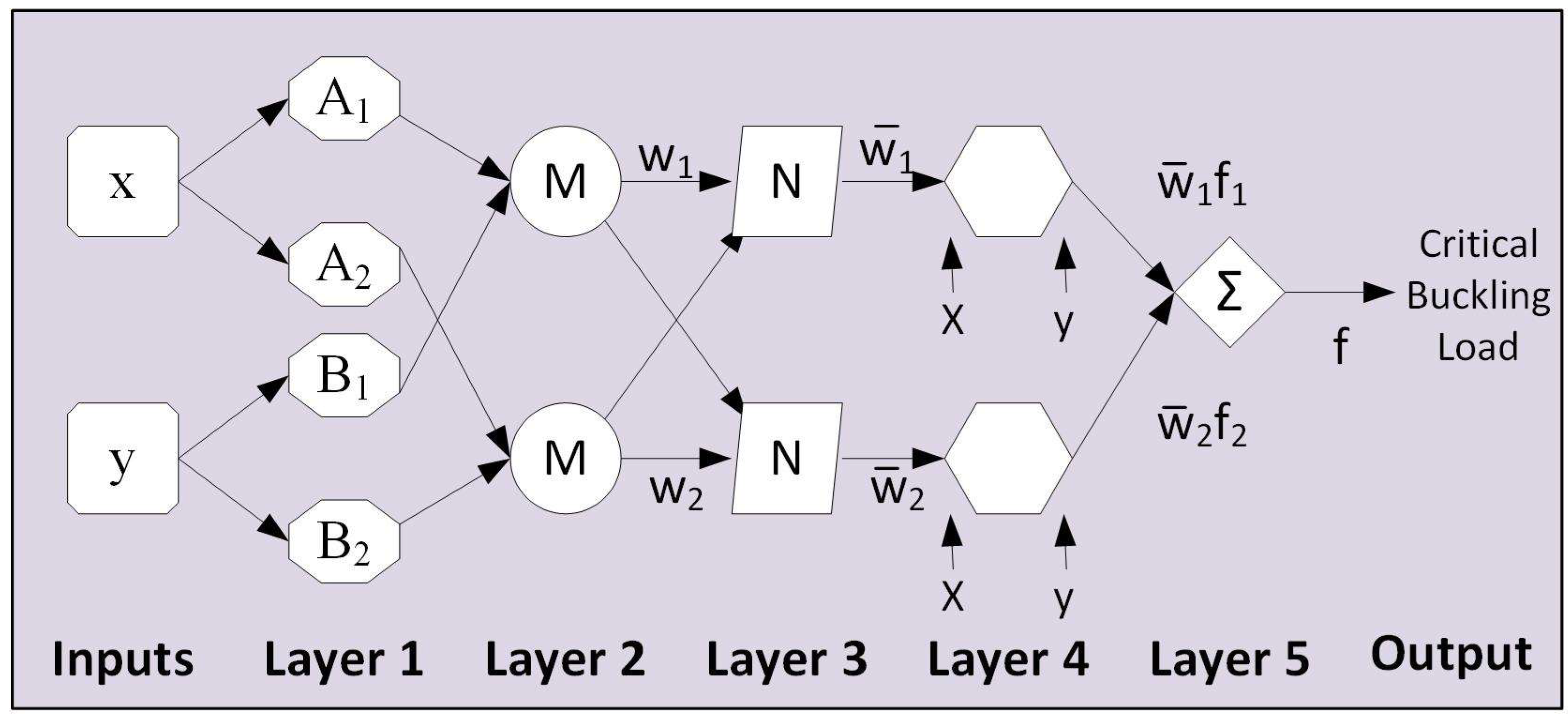
3.1.1. Adaptive Networks-Based Fuzzy Inference System

The adaptive neuro-fuzzy inference system (ANFIS) is an artificial intelligence-based algorithm developed by Jang [56] in the early 1990s. By combining features of artificial neural networks (ANN) [57,58,59] along with fuzzy logic (FL) principles, the method has a powerful potential for predicting complex non-linear processes [60,61]. The ANFIS hybrid learning algorithm could apply neural networks to optimize its algorithm, so it has a higher learning capability to adapt to its environment [62]. In the ANFIS, the number of nodes is connected by directional links in the ANN, and the fuzzy parameters of fuzzy logic algorithm can be estimated [63]. The main principle of ANFIS is to construct a set of fuzzy “if–then” rules with suitable membership functions to create the stipulated input and output variables [55]. In a specific manner, it is supposed that there are two input parameters (x and y) and one output (f). The FL-based “if–then” rules used in ANFIS can be expressed as follows [64]:

If x and y are A₁ and B₁, respectively, then f₁ = p₁x + q₁y + r₁ (Rule 1),

(1)

If x and y are A₂ and B₂, respectively, then f₂ = p₂x + q₂y + r₂ (Rule 2).

(2)

where p₁, q₁, and r₁ and p₂, q₂, and r₂ are the linear variables of Rule 1 and Rule 2, respectively, while A₁, A₂, B₁, B₂ are the functions of x and y.

Such typical ANFIS model with one output (f) and two inputs (x and y) can be visualized in Figure 1, including five main layers [56,65]:

• Layer 1: In this layer, every node is a squared node with a function as follows:

  $$O_{1,i}={\mu }_A{}_{{}_i}\left(x\right)$$

  (3)

  $$O_{1,i}={\mu }_B{}_{{}_i}\left(y\right)$$

  (4)

  where ${\mu }_A{}_{{}_i}\left(x\right)$ and ${\mu }_B{}_{{}_i}\left(y\right)$ are the membership functions of linguistic labels $A_{i\left(x\right)}$ and $B_{i\left(y\right)}$ of the inputs x and y, respectively.
• Layer 2: In this layer, every node, which is fixed, multiplies the incoming signals and sends the output:

  $$O_{2,i}={\mu }_A{}_{{}_i}\left(x\right)\times {\mu }_B{}_{{}_i}\left(y\right).$$

  (5)
• Layer 3: In this layer, every node is also fixed, and outputs of this layer are normalized as follows:

  $$O_{3,i}=\frac{w_i}{{\displaystyle {\sum }_{i=1}^2{w}_i}}.$$

  (6)
• Layer 4: Every node of this layer is an adaptive node, with the node function indicated as

  $$O_{4,i}{=\overline{\mathrm{w}}}_i\left(p_{i}x+q_{i}y+r_i\right)$$

  (7)

  where ${\mathrm{w}}_i$ infers the outputs of Layer 3, while f_i is defined by Equations (1) and (2) (I = 1, 2).
• Layer 5: In this layer, every node is a single fixed node; it sums up all incoming signals to compute the overall output as follows:

  $$O_{5,i}=\frac{{\displaystyle {\sum }_{i=1}^2{\mathrm{w}}_i{f}_i}}{{\displaystyle {\sum }_{i=1}^2{w}_i}}.$$

  (8)

3.1.2. Simulated Annealing

Simulated annealing (SA), an optimization algorithm based on the similarity between metallurgical annealing and search, is a well-known iterative metaheuristic technique for solving nonlinear and non-convex optimization problems [66]. In the SA, the annealing algorithm simulates the cooling process, which is implemented by decreasing gradually the temperature of the system, whereas the search algorithm looks for promising solutions [67]. The main advantage of the SA is that it is able to deal with arbitrary and cost functions to find an optimal solution. However, it has a disadvantage as its process is quite slow; thus, SA is a time-consuming algorithm [68]. In this study, the SA was used as a discrete technique to optimize ANFIS parameters for numerically quantifying the influence of initial geometric imperfections on the critical buckling load of structural compression members. Considering that the solution at an $i^{th}$ iteration is $x\left(i\right)$, and $f\left(x\left(i\right)\right)$ infers the relatively objective function, the subsequent solution is then expressed as follows [69]:

$$x\left(i+1\right)=\{\begin{array}{l}{x}_{new}\mathrm{if}\exp \left(\frac{-\Delta F}{T}\right)>r\\ x\left(i\right)\mathrm{otherwise}\end{array}$$

(9)

where $T$ is the temperature, $\Delta F=f\left(x_{new}\right)-f\left(x\left(i\right)\right)$ is the difference between the relevant fitness values, and $r$ is a uniform random number ranging from 0 to 1.

3.1.3. Biogeography-Based Optimization

Biogeography-based optimization (BBO) is based on the science of biogeography to study, timely and spatially, the distribution of animals and plants. This is a popular optimization technique with many important real-world applications, such as the detection of Alzheimer’s disease [70], flood susceptibility assessments [71], and predicting the consolidation coefficient of soil [72]. The main purpose of this technique is to explain the allocation of all species changing in different habitats over time [73]. Thus, it describes the evolution of new species and the migration of species between islands and the extinction of species [74]. The implementation procedure of BBO can be carried out through two main steps, namely migration and mutation [75]:

Migration is considered a probabilistic operation that uses the migration rates of an individual solution to share probabilistically the features between the solutions. The immigration rate of the ${\beta }_k$ solution of each feature $f_k$ is utilized to select whether or not to immigrate. In the case where immigration is selected, the emigrating solution, $f_j$, is selected on the base of the emigration rate:

$$f_k\left(s\right)\underset{}{\leftarrow }{f}_j\left(s\right)$$

(10)

where s is the solution feature.

Mutation is the second probabilistic operation that can modify a solution feature, where the final aim is to increase the diversification of the population.

3.1.4. Validation Criteria

In this paper, three quality assessment criteria namely the correlation coefficient (R), the root mean squared error (RMSE), and the mean absolute error (MAE) were used for validating the developed AI models. The criterion R is widely used in regression analysis [76] to estimate the linear statistical correlation between target and predicted data [41], while RMSE and MAE measure the average magnitude of the error [77,78]. The R, RMSE, and MAE calculations are expressed as [79,80,81,82]

$$R=\sqrt{\frac{{\displaystyle \sum _{j=1}^N\left(p_{0,j}-\overline{p_0}\right)\left(p_{t,j}-\overline{p_t}\right)}}{\sqrt{{{\displaystyle \sum _{j=1}^N\left(p_{0,j}-\overline{p_0}\right)}}^2{{\displaystyle \sum _{j=1}^N\left(p_{t,j}-\overline{p_t}\right)}}^2}}}$$

(11)

$$RMSE=\sqrt{\frac{1}{N}{\displaystyle \sum _{j=1}^N{(p_{0,j}-p_{t,j})}^2}}$$

(12)

$$MAE=\frac{1}{N}{\displaystyle \sum _{j=1}^N\left|p_{0,j}-p_{t,j}\right|}$$

(13)

where N is the number of the observations, $p_0$ and $\overline{p_0}$ are the measured and mean measured values of the critical buckling load, and $p_t$ and $\overline{p_t}$ are the predicted and mean predicted values of the critical buckling load, respectively.

3.2. Data Preparation

In this work, axial compression tests resulted from 57 Y-section columns, with steel with a yield strength of 420 MPa, collected by Yu et al. [83], and these tests are briefly summarized in

Table 1. Inputs and output of the present study.

N°	SLDx	SLDy	I1	I2	I3	I4	I5	I6	I7	I8	I9	Nu	φ
1	25.8	30.2	−0.28	0.32	−3.7	0.03	1.67	2.89	0.42	3.46	2.47	1523	0.906
2	26	30.2	0.42	0.49	4.02	0.05	2.15	2.73	0.64	5.43	2.14	1483	0.882
3	25.8	30.4	−0.39	0.57	2.35	0.12	−3.44	4.25	0.68	−3	5.36	1631	0.97
.	.	.	.	.	.	.	.	.	.	.	.	.	.
.	.	.	.	.	.	.	.	.	.	.	.	.	.
.	.	.	.	.	.	.	.	.	.	.	.	.	.
55	78.5	62.6	1.61	1.44	−0.96	−0.12	1	1.21	2.15	−2.09	5.92	760	0.604
56	78.9	63.6	−1.4	1.45	3.37	0.04	7.03	−6.06	2.02	−0.68	−9.69	842	0.669
57	78.1	62.6	1.09	1.52	1.97	0.31	6.1	2.53	1.85	−0.75	4.6	735	0.584
Min	25.80	23.80	−1.40	−1.34	−4.40	−0.75	−10.78	−8.25	0.42	−9.24	−9.69	735.00	0.58
Average	48.56	48.07	0.27	0.45	0.24	0.05	−0.67	1.67	1.14	−0.69	1.72	1247.51	0.86
Max	79.50	80.90	1.79	1.78	5.14	0.67	9.17	9.81	2.15	8.34	10.62	1631.00	1.02
SD*	16.28	14.83	0.84	0.84	3.16	0.29	4.33	4.54	0.53	4.76	5.23	221.01	0.09

* Standard deviation.

. In the data, all measurements of initial geometric imperfections are included. The Y-section columns were made by welding equal-leg steel angles and steel plates (Figure 2), which were manufactured from high-strength steel of 210 MPa Young’s modulus. Fifty-seven columns were fabricated with slenderness ratios (SLDs) uniformly ranging from 30 to 80 and with different width-to-thickness ratios of steel angles and plates. The columns were tested under pinned–pinned boundary condition (Figure 2). More details on the fabrication process, the geometry of the columns, and the compression test setup can be found in the original work of Yu et al. [83].

Initial imperfections of columns, such as fluctuations in mechanical properties of materials, residual stress, and initial geometric imperfections (out-of-straightness and loading eccentricity), were measured. First, the mechanical properties of steels were investigated. Tensile tests were conducted to show that the Young’s modulus varied from 210 to 211 GPa for equal angle steels and from 209 to 214 GPa for plates, whereas the yield strength ranged from 450 to 455 MPa for equal angle steels and from 485 to 496 MPa for plates. From the obtained results, it could be concluded that the fluctuations in mechanical properties are small. Second, as regards the residual stress imperfection, the results from experimental measurements showed about zero resultant force and residual stresses moments over the measured cross sections. Last but not least, initial geometric imperfections, i.e., out-of-straightness at mid-length and loading eccentricities at both ends, exhibited a significant variation with respect to the effective length of columns. From these remarks, two hypotheses could be formulated: (i) the material constituting 57 columns was assumed to be homogeneous in terms of mechanical properties and (ii) residual stress had a negligible effect on the behavior of columns under compression. The advantage of high-strength steel over normal-strength steel in decreasing the impact of residual stress over yield strength can also be found in the literature [3,11,14].

Based on the mentioned hypotheses above, input parameters for AI algorithms for predicting the buckling capacity of columns were divided into two main groups: slenderness ratios and initial geometric imperfections. Slenderness ratios (SLD) of columns containing two inputs around the x (out-of-plane) and y (in-plane) axes of the Y-section were denoted as SLD_x and SLD_y, respectively (Table 1). The out-of-plane slenderness ratio (SLD_x) varied from 25.8 to 79.50, whereas the in-plane slenderness ratio (SLD_y) varied from 23.80 to 80.90. The corresponding mean values and standard deviations were calculated and are summarized in Table 1. On the other hand, the initial geometric imperfections consisted of nine inputs. The deviation in the u-direction (Figure 2d) of the mid-length cross section (denoted by I₁ where I stands for imperfections) ranged from −1.40 to 1.79 mm. The deviation in the v-direction (Figure 2d) of the mid-length cross section (I₂) ranged from −1.34 to 1.78 mm. The rotation angle of the mid-length cross section (I₃) varied from -0.0044 to 0.00514 rad. The initial out-of-plane bending (I₄) ranged from −0.75 to 0.67 mm. The initial out-of-plane loading eccentricity at the top end (I₅) ranged from −10.78 to 9.17 mm. The initial out-of-plane loading eccentricity at the bottom end (I₆) ranged from −8.25 to 9.81 mm. The initial in-plane bending (I₇) varied from 0.42 to 2.15 mm. The initial in-plane loading eccentricity at the top end (I₈) ranged from −9.24 to 8.34 mm. The initial in-plane loading eccentricity at the bottom end (I₉) ranged from −9.69 to 10.62 mm. It is noteworthy that the initial out-of-straightness imperfections were estimated by measuring the deflections and rotation of the mid-length cross section, while assuming that the latter exposed maximum displacement for pinned–pinned columns under compression. By making these measurements, initial in-plane and out-of-plane bendings were deduced. Initial in-plane and out-of-plane loading eccentricities at the columns’ top and bottom ends were also found. The output of the prediction tools, the critical buckling load (denoted by N_u), ranged from 735 to 1631 kN with a mean value of 1247.51 kN and a standard deviation of 221.01 kN. It can be observed that the critical buckling load factor (denoted as φ), ranging from 0.58 to 1.02, exhibited an average value of 0.86 and a standard deviation of 0.09. Complete values of the dataset could be found in the work of Yu et al. [83].

In this work, the collected dataset was divided into two sets: training and testing. Training data (approximately 70% of the total data) were used to train the AI models, whereas testing data (approximately 30% of the remaining dataset) were used to quantify the performance of the AI models. Different from the original work, the training dataset (including 11 inputs and 1 output) was normalized in the [−1; 1] range. By considering all variables in a uniform range, bias within the dataset between inputs could be minimized. In this study, the range [−1; 1] was selected to better capture the non-Gaussian probability density of variables. A normalization process of parameters, such as the minimum and maximum values of the training data were performed to scale the testing dataset, as indicated in

Table 2. Normalization parameters of training data.

	SLDx	SLDy	I1	I2	I3	I3	I4	I5	I6	I7	I8	I9
Min	25.80	23.80	−1.40	−1.34	−4.31	−0.71	−10.78	−8.23	0.42	−8.46	−9.69	842.00
Max	79.50	80.70	1.75	1.78	5.14	0.67	7.03	9.81	2.05	8.34	10.62	1631.00

. The latter aims at preventing statistical correlation between training and testing dataset when normalizing. After the simulation process, a reverse transformation was applied to convert data from the normalization space to the real one.

3.3. Methodology

Figure 3 presents the methodology of the present study, in four main steps:

Step 1: Data preparation. In this step, the initial collected dataset is used for training and testing AI models such as ANFIS and ANFIS optimized with simulated annealing (ANFIS-SA) and with biogeography-based optimization (ANFIS-BBO). The training process was performed using the first 70% values of the dataset, while the testing process was done using the remaining 30% of the initial dataset. The ANFIS model was trained with the Gaussian membership function and the C-means clustering algorithm.

Step 2: Training models. In this step, the training dataset is used for training AI models, such as ANFIS, ANFIS-SA, and ANFIS-BBO.

Step 3: Validating models. In this step, the trained AI models was tested and validated using the testing dataset. For this purpose, several error criteria were employed: RMSE, MAE, and R.

Step 4: Sensitivity analysis. In this step, sensitivity analysis of inputs that affect the critical buckling load of columns was carried out. Statistical results were summarized and plotted for more quantitative and qualitative visualizations.

4. Results and Discussion

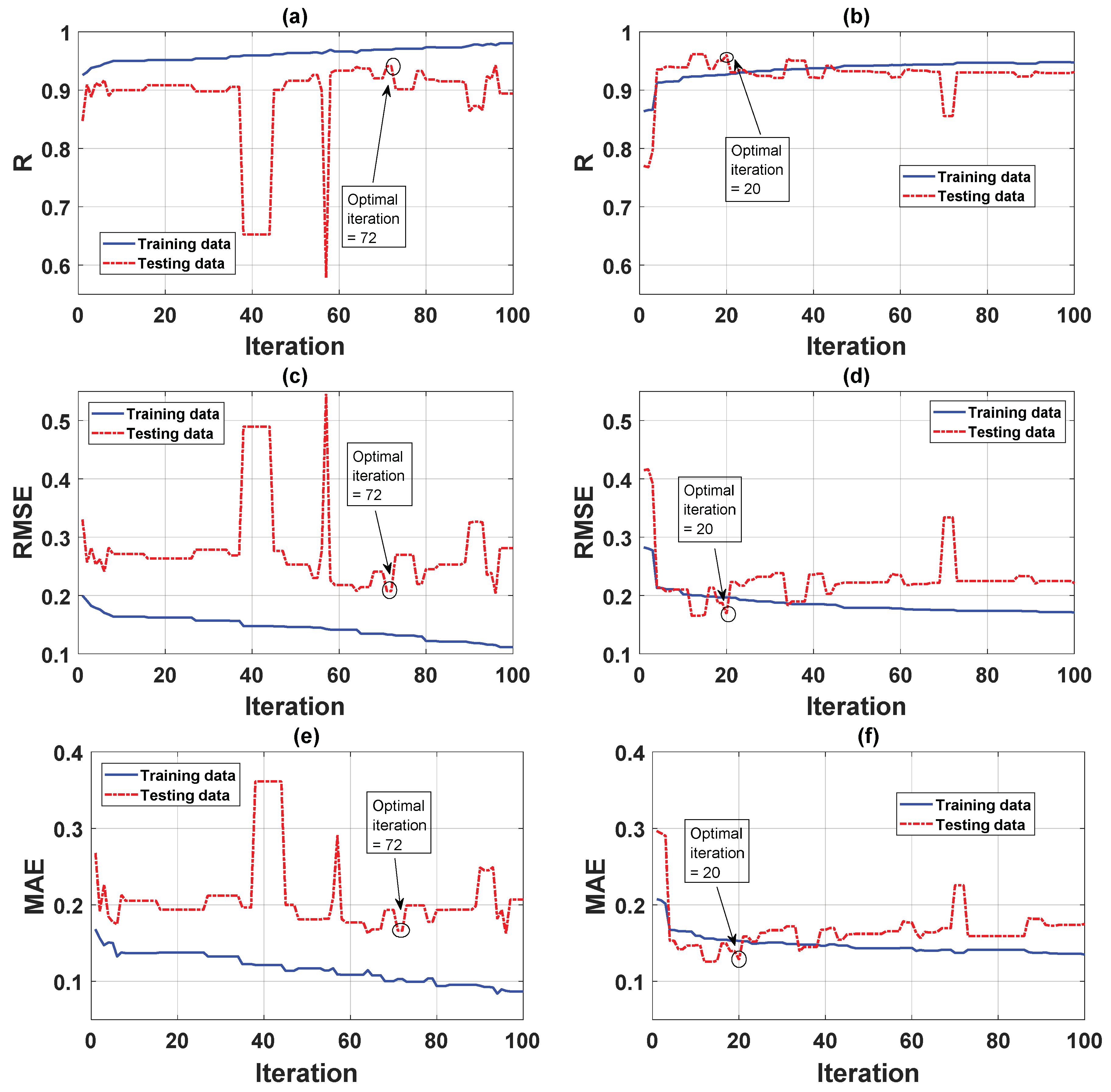
4.1. Optimization of ANFIS Parameters

The optimization procedure of consequent and antecedent ANFIS parameters using the SA and BBO techniques is presented in this section. The development of ANFIS, ANFIS-SA, and ANFIS-BBO codes were done using Matlab [84]. The population size of the SA algorithm was chosen as 25, while the number of habitats of the BBO technique was set as 50. These values were the optimal choices, deduced from trial-and-error tests. Performing with normalized data in the [−1; 1] range, the optimization procedure was investigated for 100 iterations with ANFIS-SA and ANFIS-BBO models. Figure 4 presents the optimization results in terms of R, RMSE, and MAE, showing the optimal iterations giving the highest accuracy of predicted results (i.e., the iteration when errors of the testing data started to increase). It was found that the optimal iterations were 72 and 20 using ANFIS-SA and ANFIS-BBO, respectively.

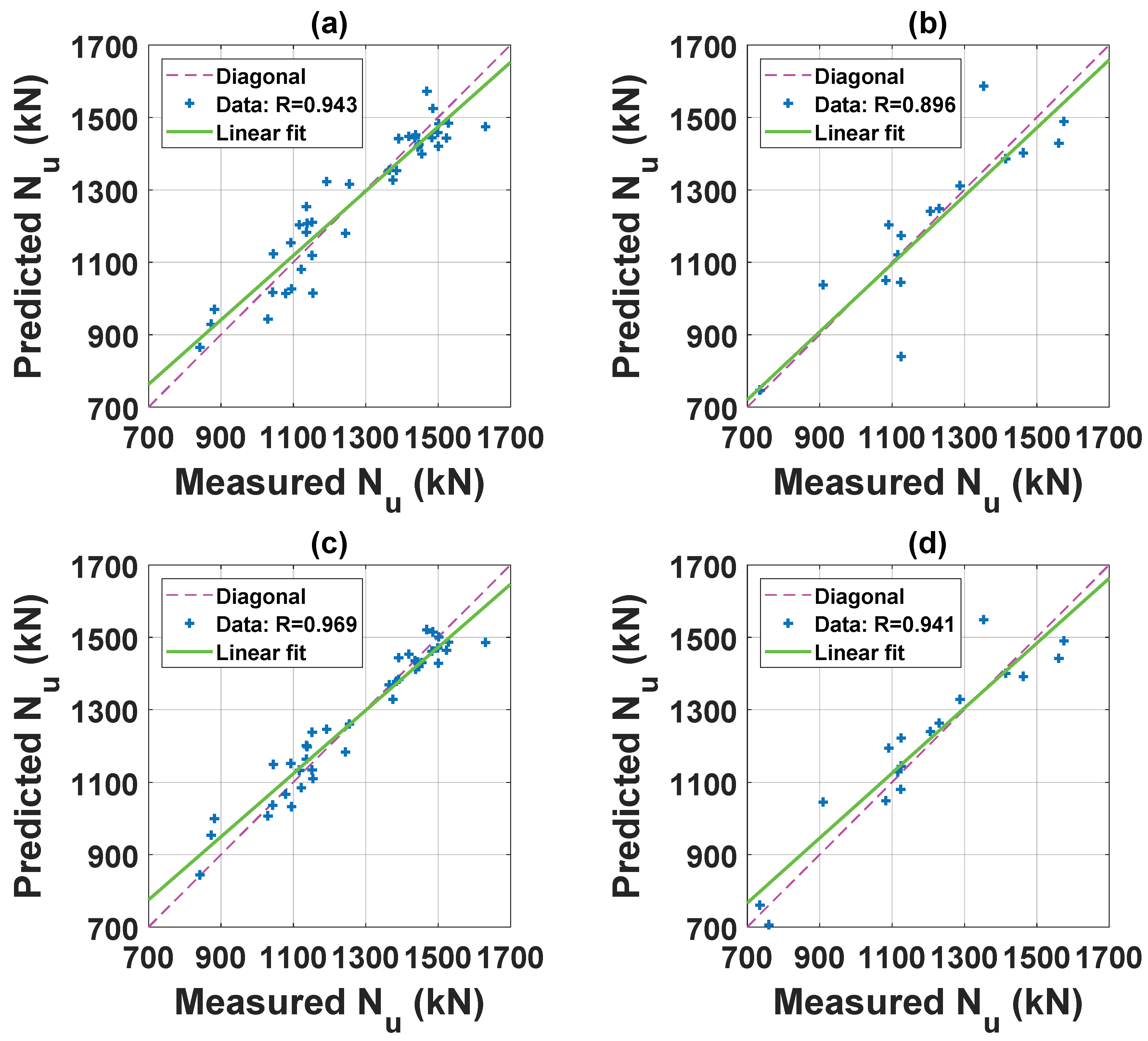
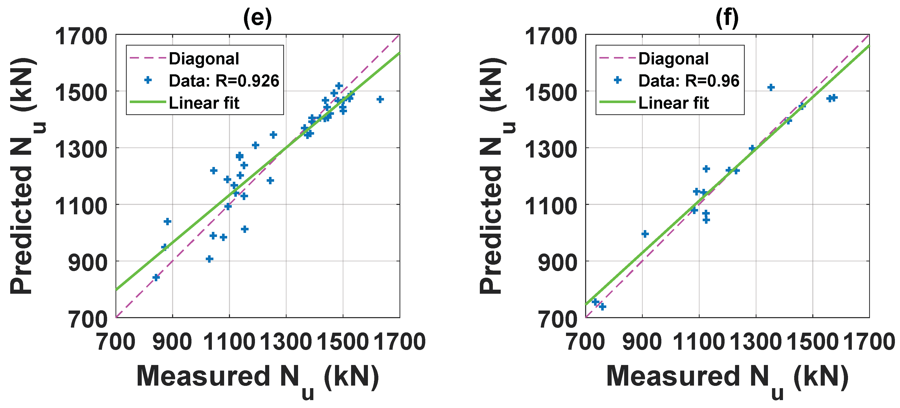
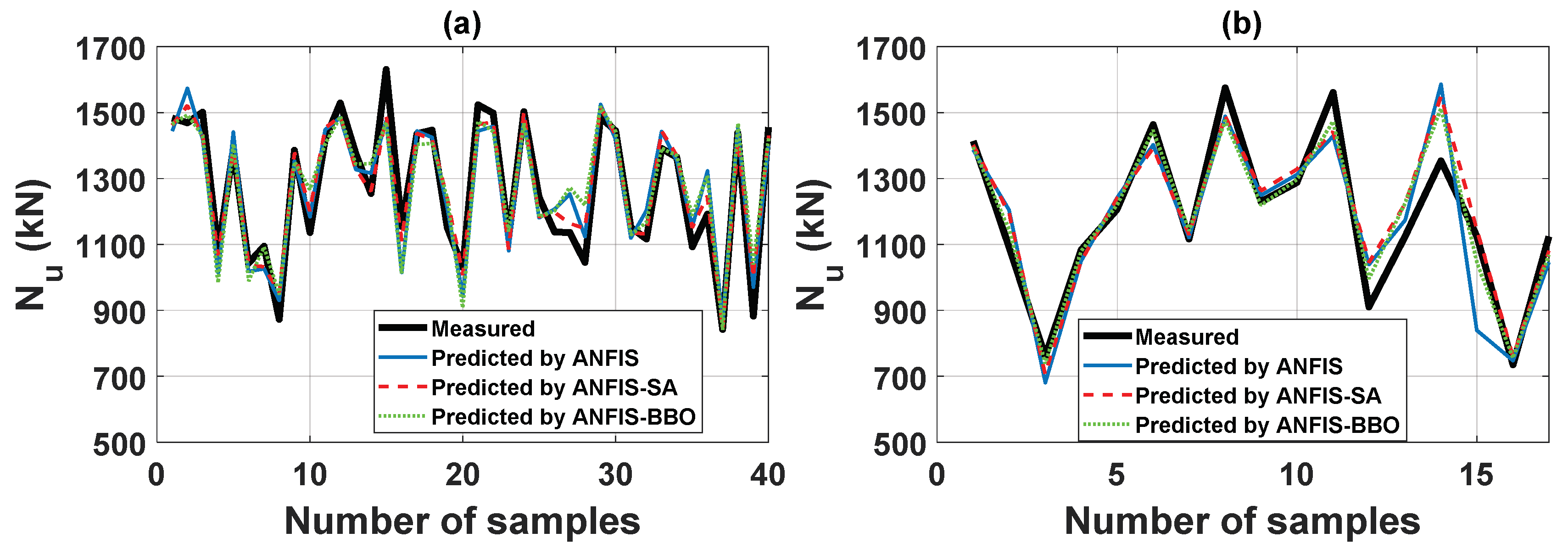
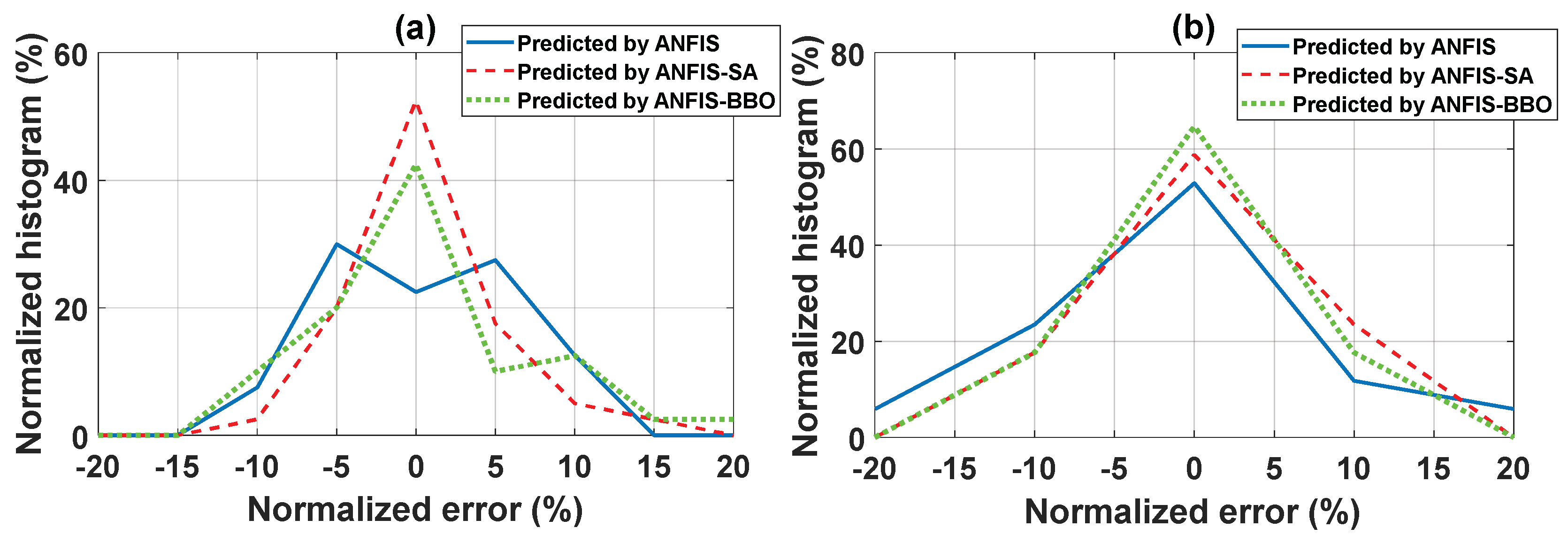
4.2. Prediction Capability

The effectiveness of ANFIS, ANFIS-SA, and ANFIS-BBO models is evaluated in this section. The results shown herein correspond to those obtained with ANFIS-SA at optimized iteration 72 and ANFIS-BBO at iteration 20. The prediction performance in a regression form is shown in Figure 5, whereas the corresponding summarized information is indicated in

Table 3. Summary of prediction capability.

Part	Method	R	RMSE (kN)	MAE (kN)	merror (kN)	StDerror (kN)	Slope	Slope Angle (°)	Intercept
Training	ANFIS	0.943	68.235	58.722	0.000	69.105	0.889	41.652	140.790
	ANFIS-SA	0.969	52.552	40.793	1.819	53.190	0.872	41.086	164.965
	ANFIS-BBO	0.926	77.692	60.437	4.441	78.553	0.837	39.944	211.516
Testing	ANFIS	0.896	111.830	82.407	−9.651	114.842	0.939	43.202	62.530
	ANFIS-SA	0.941	81.990	65.594	16.445	82.796	0.897	41.883	138.937
	ANFIS-BBO	0.960	66.558	50.723	4.363	68.459	0.916	42.482	104.257

. It is noteworthy that a reverse transformation was previously applied to obtain the final critical buckling load from the predicted normalization space. As regards the training dataset, Figure 5a,c,e present outputs N_u of ANFIS, ANFIS-SA, and ANFIS-BBO in function of the corresponding measured N_u (in kN). Figure 5b,d,f present outputs N_u of ANFIS, ANFIS-SA, and ANFIS-BBO in function of the corresponding testing data, associated with the testing part. Linear equations in the form “predicted N_u = slope * (measured N_u) + intercept” were also calculated in each case to estimate the goodness of fit between predicted and measured N_u (slope and intercept values are indicated in Table 3).

With respect to the training ANFIS, ANFIS-SA, and ANFIS-BBO parts, the slopes of 0.889, 0.872, and 0.837 were extracted, respectively. The obtained values of statistical criteria were R = 0.943, 0.969, and 0.926, RMSE = 68.235, 52.552, and 77.692, MAE = 58.722, 40.793, and 60.437, respectively. It could be deduced that ANFIS-SA is the best model for the training data. This was also confirmed by the values of the standard deviation of error StD_error (Table 3). For the training part, ANFIS-SA yielded the lowest value of StD_error compared to ANFIS and ANFIS-BBO (i.e., StD_error = 69.105, 53.190, and 78.553 for ANFIS, ANFIS-SA, and ANFIS-BBO, respectively).

Let us now consider the testing dataset. It was observed that the ANFIS-BBO model yielded the best prediction results with respect to R, RMSE, MAE, the mean of error m_error, and StD_error (i.e., R = 0.896, 0.941, 0.960; RMSE = 111.830, 81.990, 66.558; MAE = 82.407, 65.594, 50.723; m_error = −9.651, 16.445, 4.363; StD_error = 114.842, 82.796, 68.459 using ANFIS, ANFIS-SA and ANFIS-BBO, respectively). Nonetheless, the slope of the fit linear equation using ANFIS-BBO was not the smallest deviation from the diagonal line. As indicated in Table 3, the slopes were 0.939, 0.897, and 0.916 (the corresponding slope angles were 43.202°, 41.883°, and 42.482°) using ANFIS, ANFIS-SA, and ANFIS-BBO, respectively. This indicates that ANFIS gave the best result in terms of linear slope. However, ANFIS-BBO was not far, with a slope angle value only 0.7° smaller.

As observed (Figure 6a,b) for N_u values in the function of sample index, the ANFIS-BBO model might be not best for the training dataset, but its prediction performance was highest for the testing dataset. This remark was confirmed by the histograms of the normalized errors for the training dataset (Figure 7a) and for the testing dataset (Figure 7b). The normalized errors (in %) were calculated by dividing the relative errors to the measured values of N_u.

For comparison purposes, the performance of the ANFIS-SA and ANFIS-BBO models compared with the initial ANFIS is also reported.

Table 4. Increase of performance index Inc (in %) using hybrid models.

Technique	R	RMSE	MAE	StDerror
SA	5.03	26.68	20.40	27.90
BBO	7.15	40.48	38.45	40.39

indicates the comparison of prediction models with respect to R, RMSE, MAE, and StD_error, respectively. The increase of performance index, denoted as Inc, was calculated as

$$Inc=\frac{\left|W^{Hybrid}-W^{ANFIS}\right|}{W^{ANFIS}}\times 100,$$

(14)

where $W^{Hybrid}$ and $W^{ANFIS}$ were the considered criterions using hybrid and ANFIS models, respectively. It was shown that the prediction capability was increased: by 5.03% and 7.15% in terms of R; by 26.68% and 40.48% in terms of RMSE; by 20.40% and 38.45% in terms of MAE; and by 27.90% and 40.39% in terms of StD_error when using the SA and BBO optimization techniques, respectively. The SA and BBO algorithms were thus potential for improving the prediction performance of the initial ANFIS model. However, the BBO technique yielded better results. As a conclusion, from the statistical and error analysis of the prediction capability, ANFIS-BBO was the best model for the prediction of the critical buckling load of Y-section columns under compression when accounting for initial geometric imperfections.

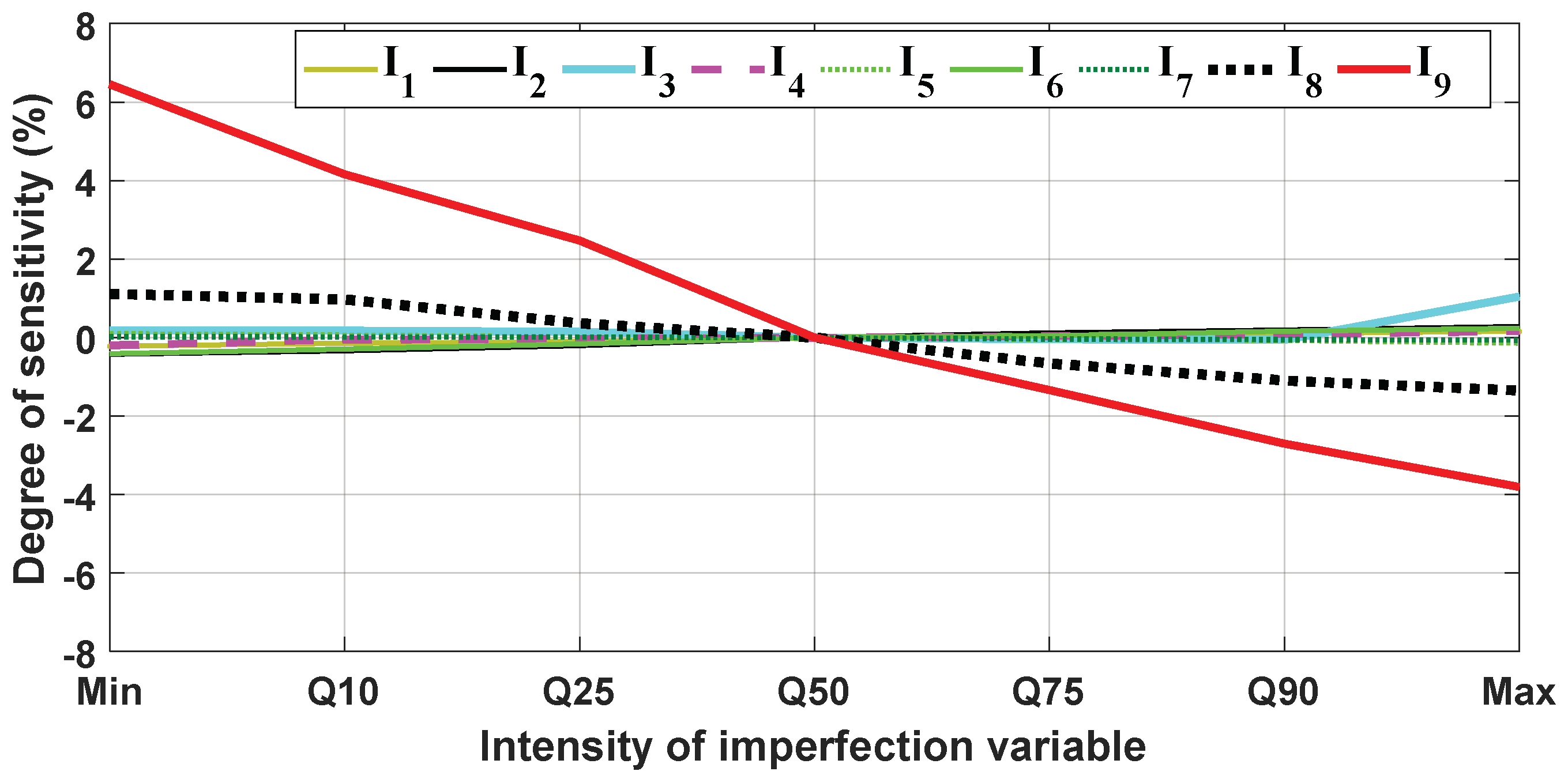
4.3. Influence of Initial Geometric Imperfections

The influence of initial geometric imperfections on the prediction of critical buckling load was studied. The selected model for the investigation was the ANFIS-BBO algorithm, as its prediction capability was proven in the previous section. In order to explore the sensitivity of each imperfection parameter, all inputs (i.e., SLD_x, SLD_y and I₁ to I₉, as indicated in Section 3.2) were used to deduce the intensity of variables, such as min, max, and quantiles Q10, Q25, Q50, Q75, Q90. The values of these parameters in the normalized space are presented in

Table 5. Intensity of input variables for sensitivity analysis in the normalized space.

Variables	Min	Q10	Q20	Q50	Q75	Q90	Max
SLDx	−1.00	−0.86	−0.76	−0.36	0.23	0.63	1.00
SLDy	−1.00	−0.78	−0.66	−0.20	0.15	0.64	1.00
I1	−1.00	−0.61	−0.37	0.16	0.37	0.70	1.00
I2	−1.00	−0.75	−0.37	0.19	0.52	0.75	1.00
I3	−1.00	−0.94	−0.71	0.35	0.59	0.74	1.00
I4	−1.00	−0.20	−0.07	0.07	0.31	0.59	1.00
I5	−1.00	−0.64	−0.17	0.05	0.42	0.70	1.00
I6	−1.00	−0.64	−0.22	0.25	0.40	0.79	1.00
I7	−1.00	−0.85	−0.75	−0.34	0.36	0.69	1.00
I8	−1.00	−0.89	−0.39	−0.09	0.44	0.79	1.00
I9	−1.00	−0.55	−0.22	0.26	0.52	0.79	1.00

.

In the sensitivity analysis, each input was varied from its lowest to highest intensity values, while the median Q50 values were applied to all other variables. Thereby, the degree of sensitivity, denoted as DoS (in %), of the considered input variable could be calculated as follows:

$$Do{S}_i^j=\frac{N_i^j-N_{Q50}^{all}}{N_{Q50}^{all}}\times 100,$$

(15)

where $N_{Q50}^{all}$ was the output critical buckling load when all input variables remained at their median values. $N_i^j$ was the output critical buckling load when applying input number j at its intensity i, and $Do{S}_i^j$ was the associated degree of sensitivity of the input j (I = 1, …, 7 and j = 1, …, 9). Figure 8 presents the calculated degrees of sensitivity of all imperfection parameters. It can be clearly seen that the initial in-plane loading eccentricity at the bottom end (I₉) had the highest impact on the prediction of critical buckling load. The degree of sensitivity of I₉ ranged from 4 to 6.5%, when varying I₉ from the highest to lowest level of values. The second input that exhibited a significant effect on the critical buckling load prediction was the initial in-plane loading eccentricity at the top end (I₈). Its degree of sensitivity varied from −1.5 to 1%, when ranging I₈ from its highest to lowest values. All other imperfections had a similar effect and varied in ranges so small that the influences could be neglected. A summary of sensitivity analysis is indicated in

Table 6. Summary of the degree of sensitivity (in %) of input variables at different intensity values.

Variables	Min	Q10	Q25	Q50	Q75	Q90	Max
I1	−0.219	−0.145	−0.100	0	0.041	0.102	0.159
I2	−0.416	−0.329	−0.195	0	0.116	0.195	0.284
I3	0.185	0.177	0.146	0	−0.032	−0.053	1.054
I4	−0.194	−0.049	−0.025	0	0.043	0.093	0.168
I5	0.103	0.067	0.021	0	−0.036	−0.064	−0.133
I6	−0.401	−0.285	−0.151	0	0.048	0.172	0.240
I7	0.029	0.022	0.018	0	−0.031	−0.046	−0.059
I8	1.118	0.976	0.368	0	−0.655	−1.093	−1.348
I9	6.467	4.160	2.468	0	−1.329	−2.706	−3.798
SLDx	32.501	25.259	20.112	0	−25.692	−50.995	−69.868
SLDy	−32.845	−23.565	−18.997	0	−8.743	34.658	49.667

. From the original data, it was observed that the critical buckling load factor (φ) ranged from 0.58 to 1.02, exhibited an average value of 0.86, and a standard deviation of 0.09 (Table 1). This indicated that the instability was almost predicted when applying compression loading to columns. The actual buckling capacity of columns was reduced with an average value of 14%. It was also noticed that, when the slenderness of columns increases, the values of the critical buckling load factor decrease (e.g., for specimens from N°55 to 57). This meant that initial imperfections, by largely changing the capacity of columns under compression, played an important role. They needed to be taken into account in the modeling as their influence became relevant. The next section is dedicated to an analysis of the influence of slenderness ratios on the predicted results.

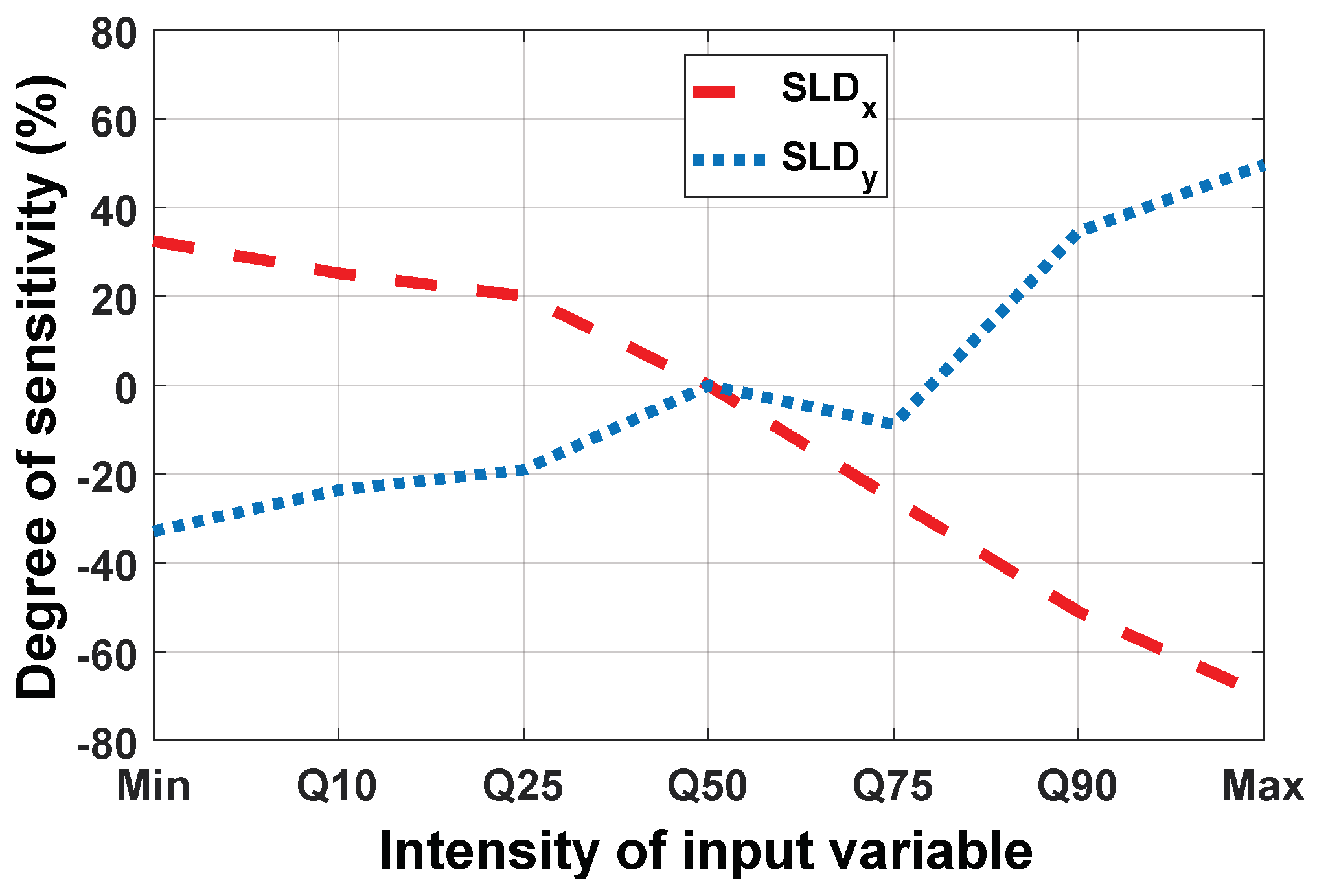
4.4. Influence of Slenderness

Similar sensitivity analysis was performed for slenderness ratios SLD_x and SLD_y. Figure 9 presents the degree of sensitivity of SLD_x and SLD_y, whereas summary information is indicated in Table 6. The degree of sensitivity of SLD_x varied from −70 to 32% when applying the highest to lowest values. As regards SLD_y, the degree of sensitivity varied from −32 to 49% when applying the lowest to highest values. It can be deduced that both slenderness ratios exhibited important effects on the prediction of the critical buckling load, and the effects were more important than those of the initial imperfections, as calculated in the previous section. This fact is relevant, as shown in Euler’s formula for estimating the critical buckling load [85,86,87] under zero imperfections.

As a conclusion, the developed ANFIS-BBO model in this study exhibited a strong capability for the prediction of the critical buckling load of Y-section columns under compression. Quantitative influence of initial geometric imperfections in both out-of-plane and in-plane directions was also deduced using such an ANFIS-BBO model. The ANFIS-BBO model could thus be a robust and useful numerical tool for analyzing the problem of column instability.

5. Conclusions

In this work, a methodology modeling for numerically quantifying the influence of initial geometric imperfections on the critical buckling load of structural compression members based on the use of hybrid AI models was proposed. The methodology was based on the improvement of the ANFIS by different metaheuristic optimization techniques such as SA and BBO, for the prediction problem of column instability. The developed hybrid AI models were trained and validated based on experimental tests available in the literature. Results showed that the BBO optimization algorithm yielded the best results with respect to all commonly used statistical criteria, such as R, RMSE, and MAE, respectively. After sensitivity analysis, geometric imperfections that exhibited a major impact on column compression capacity were deduced, such as the initial in-plane loading eccentricity at both top and bottom ends. However, in further investigations, other initial imperfections, such as fluctuations in mechanical properties of materials as well as residual stresses, should be taken into account in order to quantify the influence of these parameters. The methodology could also be applied to investigate other structural elements of different cross sections in order to generalize the influence of initial in-plane and out-of-plane geometric imperfections. An empirical equation accounting for initial imperfections should also be derived based on the developed numerical prediction model in order to facilitate the use in engineering applications. Finally, AI approaches coupled with finite element analysis could be a potential candidate for studying a nonlinear post-buckling regime of columns in further researches.

References

1. Abramovich, H. Stability and Vibrations of Thin-Walled Composite Structures, 1st ed.; Woodhead Publishing: Cambridge, UK, 2017. [Google Scholar]
2. Quach, W.M.; Teng, J.G.; Chung, K.F. Effect of the manufacturing process on the behaviour of press-braked thin-walled steel columns. Eng. Struct. 2010, 32, 3501–3515. [Google Scholar] [CrossRef]
3. Shi, G.; Zhou, W.J.; Bai, Y.; Lin, C.C. Local buckling of 460 MPa high strength steel welded section stub columns under axial compression. J. Constr. Steel Res. 2014, 100, 60–70. [Google Scholar] [CrossRef]
4. Šmak, M.; Straka, B. Geometrical and Structural Imperfections of Steel Member Systems. Procedia Eng. 2012, 40, 434–439. [Google Scholar] [CrossRef] [Green Version]
5. Pastor, M.M.; Bonada, J.; Roure, F.; Casafont, M. Residual stresses and initial imperfections in non-linear analysis. Eng. Struct. 2013, 46, 493–507. [Google Scholar] [CrossRef]
6. Ma, T.-Y.; Liu, X.; Hu, Y.-F.; Chung, K.-F.; Li, G.-Q. Structural behaviour of slender columns of high strength S690 steel welded H-sections under compression. Eng. Struct. 2018, 157, 75–85. [Google Scholar] [CrossRef]
7. Shi, G.; Jiang, X.; Zhou, W.J.; Chan, T.M.; Zhang, Y. Experimental study on column buckling of 420 MPa high strength steel welded circular tubes. J. Constr. Steel Res. 2014, 100, 71–81. [Google Scholar] [CrossRef]
8. Ban, H.; Shi, G.; Shi, Y.; Wang, Y. Overall buckling behavior of 460MPa high strength steel columns: Experimental investigation and design method. J. Constr. Steel Res. 2012, 74, 140–150. [Google Scholar] [CrossRef]
9. Kim, D.-K.; Lee, C.-H.; Han, K.-H.; Kim, J.-H.; Lee, S.-E.; Sim, H.-B. Strength and residual stress evaluation of stub columns fabricated from 800MPa high-strength steel. J. Constr. Steel Res. 2014, 102, 111–120. [Google Scholar] [CrossRef]
10. Shi, G.; Xu, K.; Ban, H.; Lin, C. Local buckling behavior of welded stub columns with normal and high strength steels. J. Constr. Steel Res. 2016, 119, 144–153. [Google Scholar] [CrossRef]
11. Ban, H.; Shi, G.; Shi, Y.; Wang, Y. Residual Stress Tests of High-Strength Steel Equal Angles. J. Struct. Eng. 2012, 138, 1446–1454. [Google Scholar] [CrossRef]
12. Ban, H.Y.; Shi, G.; Shi, Y.J.; Wang, Y.Q. Column buckling tests of 420 MPa high strength steel single equal angles. Int. J. Str. Stab. Dyn. 2013, 13, 1250069. [Google Scholar] [CrossRef]
13. Cao, K.; Guo, Y.-J.; Zeng, D.-W. Buckling behavior of large-section and 420 MPa high-strength angle steel columns. J. Constr. Steel Res. 2015, 111, 11–20. [Google Scholar] [CrossRef]
14. Cao, X.; Xu, Y.; Kong, Z.; Shen, H.; Zhong, W. Residual stress of 800 MPa high strength steel welded T section: Experimental study. J. Constr. Steel Res. 2017, 131, 30–37. [Google Scholar] [CrossRef]
15. Khot, N.S. On the Influence of Initial Geometric Imperfections on the Buckling and Postbuckling Behavior of Fiber-Reinforced Cylindrical Shells under Uniform Axial Compression; Air Force Flight Dynamics Lab: Wright-Patterson AFB, OH, USA, 1968. [Google Scholar]
16. Zhao, C.; Niu, J.; Zhang, Q.; Zhao, C.; Xie, J. Buckling behavior of a thin-walled cylinder shell with the cutout imperfections. Mech. Adv. Mater. Struct. 2018, 1–7. [Google Scholar] [CrossRef]
17. Sadovský, Z.; Kriváček, J.; Ivančo, V.; Ďuricová, A. Computational modelling of geometric imperfections and buckling strength of cold-formed steel. J. Constr. Steel Res. 2012, 78, 1–7. [Google Scholar] [CrossRef]
18. Bonada, J.; Casafont, M.; Roure, F.; Pastor, M.M. Selection of the initial geometrical imperfection in nonlinear FE analysis of cold-formed steel rack columns. Thin-Walled Struct. 2012, 51, 99–111. [Google Scholar] [CrossRef]
19. Gendy, B.L.; Hanna, M.T. Effect of geometric imperfections on the ultimate moment capacity of cold-formed sigma-shape sections. HBRC J. 2017, 13, 163–170. [Google Scholar] [CrossRef] [Green Version]
20. Tomás, A.; Tovar, J.P. The influence of initial geometric imperfections on the buckling load of single and double curvature concrete shells. Comput. Struct. 2012, 96–97, 34–45. [Google Scholar] [CrossRef]
21. Vu, L.H.; Duc, N.C.; Dong, L.V.; Truong, D.L.; Anh, N.M.T.; Hung, H.Q.; Hue, P.V. Load Rating and Buckling of Circular Concrete-Filled Steel Tube (CFST): Simulation and Experiment. IOP Conf. Ser. Mater. Sci. Eng. 2018, 371, 012032. [Google Scholar] [CrossRef]
22. Lai, B.; Richard Liew, J.Y.; Wang, T. Buckling behaviour of high strength concrete encased steel composite columns. J. Constr. Steel Res. 2019, 154, 27–42. [Google Scholar] [CrossRef]
23. Shahrjerdi, A.; Bahramibabamiri, B. The effect of different geometrical imperfection of buckling of composite cylindrical shells subjected to axial loading. Int. J. Mech. Mater. Eng. 2015, 10, 6. [Google Scholar] [CrossRef]
24. Niu, P.; Yang, G.; Jin, C.F.; Li, X. Influence of the Initial Imperfection on the Buckling of Steel Member Wrapped by Carbon Fibre. Appl. Mech. Mater. 2012, 166–169, 738–742. [Google Scholar] [CrossRef]
25. Wstawska, I. The influence of geometric imperfections on the stability of three-layer beams with foam core. Arch. Mech. Technol. Mater. 2017, 37, 65–69. [Google Scholar] [CrossRef] [Green Version]
26. Damanpack, A.R.; Bodaghi, M.; Liao, W.H. Snap buckling of NiTi tubes. Int. J. Solids Struct. 2018, 146, 29–42. [Google Scholar] [CrossRef]
27. Jiang, D.; Bechle, N.J.; Landis, C.M.; Kyriakides, S. Buckling and recovery of NiTi tubes under axial compression. Int. J. Solids Struct. 2016, 80, 52–63. [Google Scholar] [CrossRef]
28. Szymczak, C.; Kujawa, M. Flexural buckling and post-buckling of columns made of aluminium alloy. Eur. J. Mech. A/Solids 2019, 73, 420–429. [Google Scholar] [CrossRef]
29. Liu, M.; Zhang, L.; Wang, P.; Chang, Y. Buckling behaviors of section aluminum alloy columns under axial compression. Eng. Struct. 2015, 95, 127–137. [Google Scholar] [CrossRef]
30. Dao, H.B.; Dao, V.D.; Vu, H.N.; Nguyen, T.P. Nonlinear static and dynamic buckling analysis of imperfect eccentrically stiffened functionally graded circular cylindrical thin shells under axial compression. Int. J. Mech. Sci. 2013, 74, 190–200. [Google Scholar]
31. Vu, H.N.; Nguyen, T.P.; Dao, H.B. Buckling analysis of parallel eccentrically stiffened functionally graded annular spherical segments subjected to mechanic loads. Mech. Adv. Mater. Struct. 2018, 1–10. [Google Scholar] [CrossRef]
32. Tomar, S.S.; Talha, M. Thermo-Mechanical Buckling Analysis of Functionally Graded Skew Laminated Plates with Initial Geometric Imperfections. Int. J. Appl. Mech. 2018, 10, 1850014. [Google Scholar] [CrossRef]
33. Dou, C.; Pi, Y.L. Effects of Geometric Imperfections on Flexural Buckling Resistance of Laterally Braced Columns. J. Struct. Eng. 2016, 142, 04016048. [Google Scholar] [CrossRef]
34. Crisfield, M. A fast incremental/iterative solution procedure that handles “snap-through”. In Computational Methods in Nonlinear Structural and Solid Mechanics; Elsevier: Amsterdam, The Netherlands, 1981; pp. 55–62. [Google Scholar]
35. Crisfield, M.A. A faster modified newton-raphson iteration. Comput. Methods Appl. Mech. Eng. 1979, 20, 267–278. [Google Scholar] [CrossRef]
36. Saffari, H.; Fadaee, M.J.; Tabatabaei, R. Nonlinear analysis of space trusses using modified normal flow algorithm. J. Struct. Eng. 2008, 134, 998–1005. [Google Scholar] [CrossRef]
37. Valeš, J.; Kala, Z. Mesh convergence study of solid FE model for buckling analysis. AIP Conf. Proc. 2018, 1978, 150005. [Google Scholar]
38. Ellobody, E. Finite Element Analysis and Design of Steel and Steel–Concrete Composite Bridges; Butterworth-Heinemann: Amsterdam, The Netherlands; Boston, MA, USA, 2014; ISBN 978-0-12-417247-0. [Google Scholar]
39. Crisfield, M.A.; Remmers, J.J.; Verhoosel, C.V. Nonlinear Finite Element Analysis of Solids and Structures; John Wiley & Sons: Hoboken, NJ, USA, 1997. [Google Scholar]
40. Stoffel, M.; Bamer, F.; Markert, B. Artificial neural networks and intelligent finite elements in non-linear structural mechanics. Thin-Walled Struct. 2018, 131, 102–106. [Google Scholar] [CrossRef]
41. Le, L.M.; Ly, H.-B.; Pham, B.T.; Le, V.M.; Pham, T.A.; Nguyen, D.-H.; Tran, X.-T.; Le, T.-T. Hybrid Artificial Intelligence Approaches for Predicting Buckling Damage of Steel Columns Under Axial Compression. Materials 2019, 12, 1670. [Google Scholar] [CrossRef]
42. Chen, H.; Asteris, P.G.; Jahed Armaghani, D.; Gordan, B.; Pham, B.T. Assessing Dynamic Conditions of the Retaining Wall: Developing Two Hybrid Intelligent Models. Appl. Sci. 2019, 9, 1042. [Google Scholar] [CrossRef]
43. Asteris, P.G.; Tsaris, A.K.; Cavaleri, L.; Repapis, C.C.; Papalou, A.; Di Trapani, F.; Karypidis, D.F. Prediction of the Fundamental Period of Infilled RC Frame Structures Using Artificial Neural Networks. Intell. Neurosci. 2016, 2016, 20. [Google Scholar] [CrossRef]
44. Asteris, P.G.; Kolovos, K.G.; Douvika, M.G.; Roinos, K. Prediction of self-compacting concrete strength using artificial neural networks. Eur. J. Environ. Civ. Eng. 2016, 20, s102–s122. [Google Scholar] [CrossRef]
45. Asteris, P.G.; Plevris, V. Anisotropic masonry failure criterion using artificial neural networks. Neural Comput. Appl. 2017, 28, 2207–2229. [Google Scholar] [CrossRef]
46. Asteris, P.G.; Roussis, P.C.; Douvika, M.G. Feed-Forward Neural Network Prediction of the Mechanical Properties of Sandcrete Materials. Sensors 2017, 17, 1344. [Google Scholar] [CrossRef]
47. Asteris, P.G.; Kolovos, K.G. Self-compacting concrete strength prediction using surrogate models. Neural Comput. Appl. 2019, 31, 409–424. [Google Scholar] [CrossRef]
48. Jimenez-Martinez, M.; Alfaro-Ponce, M. Fatigue damage effect approach by artificial neural network. Int. J. Fatigue 2019, 124, 42–47. [Google Scholar] [CrossRef]
49. Didych, I.S.; Pastukh, O.; Pyndus, Y.; Yasniy, O. The evaluation of durability of structural elements using neural networks. Acta Met. Slovaca 2018, 24, 82–87. [Google Scholar] [CrossRef]
50. Ali, F.; McKinney, J. Artificial Neural Networks for the Spalling Classification & Failure Prediction Times of High Strength Concrete Columns. Fire Eng. 2014, 5, 203–214. [Google Scholar]
51. Kumar, M.; Yadav, N. Buckling analysis of a beam–column using multilayer perceptron neural network technique. J. Frankl. Inst. 2013, 350, 3188–3204. [Google Scholar] [CrossRef]
52. Mandal, P. Artificial neural network prediction of buckling load of thin cylindrical shells under axial compression. Eng. Struct. 2017, 152, 843–855. [Google Scholar]
53. Hasanzadehshooiili, H.; Lakirouhani, A.; Šapalas, A. Neural network prediction of buckling load of steel arch-shells. Arch. Civ. Mech. Eng. 2012, 12, 477–484. [Google Scholar] [CrossRef]
54. Mallela, U.K.; Upadhyay, A. Buckling load prediction of laminated composite stiffened panels subjected to in-plane shear using artificial neural networks. Thin-Walled Struct. 2016, 102, 158–164. [Google Scholar] [CrossRef]
55. Bilgehan, M. Comparison of ANFIS and NN models—With a study in critical buckling load estimation. Appl. Soft Comput. 2011, 11, 3779–3791. [Google Scholar] [CrossRef]
56. Jang, J.-R. ANFIS: Adaptive-network-based fuzzy inference system. IEEE Trans. Syst. Man Cybern. 1993, 23, 665–685. [Google Scholar] [CrossRef]
57. Asteris, P.G.; Nozhati, S.; Nikoo, M.; Cavaleri, L.; Nikoo, M. Krill herd algorithm-based neural network in structural seismic reliability evaluation. Mech. Adv. Mater. Struct. 2018, 1–8. [Google Scholar] [CrossRef]
58. Asteris, P.G.; Nikoo, M. Artificial bee colony-based neural network for the prediction of the fundamental period of infilled frame structures. Neural Comput. Appl. 2019. [Google Scholar] [CrossRef]
59. Plevris, V.; Asteris, P.G. Modeling of masonry failure surface under biaxial compressive stress using Neural Networks. Constr. Build. Mater. 2014, 55, 447–461. [Google Scholar] [CrossRef]
60. Mekanik, F.; Imteaz, M.A.; Talei, A. Seasonal rainfall forecasting by adaptive network-based fuzzy inference system (ANFIS) using large scale climate signals. Clim. Dyn. 2016, 46, 3097–3111. [Google Scholar] [CrossRef]
61. Nguyen, V.V.; Pham, B.T.; Vu, B.T.; Prakash, I.; Jha, S.; Shahabi, H.; Shirzadi, A.; Ba, D.N.; Kumar, R.; Chatterjee, J.M.; et al. Hybrid Machine Learning Approaches for Landslide Susceptibility Modeling. Forests 2019, 10, 157. [Google Scholar] [CrossRef]
62. Jang, J.-S.R. Neuro-Fuzzy and Soft Computing: A Computational Approach to Learning and Machine Intelligence; Prentice Hall: Englewool Cliffs, NJ, USA, 1997; ISBN 978-0-13-261066-7. [Google Scholar]
63. Azadeh, A.; Asadzadeh, S.M.; Ghanbari, A. An adaptive network-based fuzzy inference system for short-term natural gas demand estimation: Uncertain and complex environments. Energy Policy 2010, 38, 1529–1536. [Google Scholar] [CrossRef]
64. Güler, İ.; Übeyli, E.D. Adaptive neuro-fuzzy inference system for classification of EEG signals using wavelet coefficients. J. Neurosci. Methods 2005, 148, 113–121. [Google Scholar] [CrossRef]
65. Chen, W.; Panahi, M.; Tsangaratos, P.; Shahabi, H.; Ilia, I.; Panahi, S.; Li, S.; Jaafari, A.; Ahmad, B.B. Applying population-based evolutionary algorithms and a neuro-fuzzy system for modeling landslide susceptibility. Catena 2019, 172, 212–231. [Google Scholar] [CrossRef]
66. Wei, L.; Zhang, Z.; Zhang, D.; Leung, S.C.H. A simulated annealing algorithm for the capacitated vehicle routing problem with two-dimensional loading constraints. Eur. J. Oper. Res. 2018, 265, 843–859. [Google Scholar] [CrossRef]
67. Florios, K. A hyperplanes intersection simulated annealing algorithm for maximum score estimation. Econ. Stat. 2018, 8, 37–55. [Google Scholar] [CrossRef]
68. Krishnaraj, J.; Pugazhendhi, S.; Rajendran, C.; Thiagarajan, S. Simulated annealing algorithms to minimise the completion time variance of jobs in permutation flowshops. Int. J. Ind. Syst. Eng. 2019, 31, 425–451. [Google Scholar] [CrossRef]
69. Zhang, W.; Maleki, A.; Rosen, M.A.; Liu, J. Optimization with a simulated annealing algorithm of a hybrid system for renewable energy including battery and hydrogen storage. Energy 2018, 163, 191–207. [Google Scholar] [CrossRef]
70. Wang, S.-H.; Zhang, Y.; Li, Y.-J.; Jia, W.-J.; Liu, F.-Y.; Yang, M.-M.; Zhang, Y.-D. Single slice based detection for Alzheimer’s disease via wavelet entropy and multilayer perceptron trained by biogeography-based optimization. Multimedia Tools Appl. 2018, 77, 10393–10417. [Google Scholar] [CrossRef]
71. Ahmadlou, M.; Karimi, M.; Alizadeh, S.; Shirzadi, A.; Parvinnejhad, D.; Shahabi, H.; Panahi, M. Flood susceptibility assessment using integration of adaptive network-based fuzzy inference system (ANFIS) and biogeography-based optimization (BBO) and BAT algorithms (BA). Geocarto Int. 2018, 1–21. [Google Scholar] [CrossRef]
72. Pham, B.T.; Nguyen, M.D.; Bui, K.-T.T.; Prakash, I.; Chapi, K.; Bui, D.T. A novel artificial intelligence approach based on Multi-layer Perceptron Neural Network and Biogeography-based Optimization for predicting coefficient of consolidation of soil. Catena 2019, 173, 302–311. [Google Scholar] [CrossRef]
73. Li, L.-L.; Yang, Y.-F.; Wang, C.-H.; Lin, K.-P. Biogeography-based optimization based on population competition strategy for solving the substation location problem. Expert Syst. Appl. 2018, 97, 290–302. [Google Scholar] [CrossRef]
74. Jaafari, A.; Panahi, M.; Pham, B.T.; Shahabi, H.; Bui, D.T.; Rezaie, F.; Lee, S. Meta optimization of an adaptive neuro-fuzzy inference system with grey wolf optimizer and biogeography-based optimization algorithms for spatial prediction of landslide susceptibility. Catena 2019, 175, 430–445. [Google Scholar] [CrossRef]
75. Mirjalili, S. Biogeography-Based Optimisation. In Evolutionary Algorithms and Neural Networks; Springer: Berlin, Germany, 2019; pp. 57–72. [Google Scholar]
76. Menard, S. Coefficients of Determination for Multiple Logistic Regression Analysis. Am. Stat. 2000, 54, 17–24. [Google Scholar]
77. Chai, T.; Draxler, R.R. Root mean square error (RMSE) or mean absolute error (MAE)?—Arguments against avoiding RMSE in the literature. Geosci. Model Dev. 2014, 7, 1247–1250. [Google Scholar] [CrossRef]
78. Dao, D.V.; Trinh, S.H.; Ly, H.-B.; Pham, B.T. Prediction of Compressive Strength of Geopolymer Concrete Using Entirely Steel Slag Aggregates: Novel Hybrid Artificial Intelligence Approaches. Appl. Sci. 2019, 9, 1113. [Google Scholar] [CrossRef]
79. Dao, D.V.; Ly, H.-B.; Trinh, S.H.; Le, T.-T.; Pham, B.T. Artificial Intelligence Approaches for Prediction of Compressive Strength of Geopolymer Concrete. Materials 2019, 12, 983. [Google Scholar] [CrossRef]
80. Willmott, C.J.; Matsuura, K. Advantages of the mean absolute error (MAE) over the root mean square error (RMSE) in assessing average model performance. Clim. Res. 2005, 30, 79–82. [Google Scholar] [CrossRef]
81. Ly, H.-B.; Monteiro, E.; Le, T.-T.; Le, V.M.; Dal, M.; Regnier, G.; Pham, B.T. Prediction and Sensitivity Analysis of Bubble Dissolution Time in 3D Selective Laser Sintering Using Ensemble Decision Trees. Materials 2019, 12, 1544. [Google Scholar] [CrossRef]
82. Pham, B.T.; Nguyen, M.D.; Dao, D.V.; Prakash, I.; Ly, H.-B.; Le, T.-T.; Ho, L.S.; Nguyen, K.T.; Ngo, T.Q.; Hoang, V.; et al. Development of artificial intelligence models for the prediction of Compression Coefficient of soil: An application of Monte Carlo sensitivity analysis. Sci. Total Environ. 2019, 679, 172–184. [Google Scholar] [CrossRef]
83. Yu, X.; Deng, H.; Zhang, D.; Cui, L. Buckling behavior of 420MPa HSSY columns: Test investigation and design approach. Eng. Struct. 2017, 148, 793–812. [Google Scholar] [CrossRef]
84. The MathWorks. MATLAB; The MathWorks: Natick, MA, USA, 2018. [Google Scholar]
85. Timoshenko, S.P.; Gere, J.M. Theory of Elastic Stability; McGraw-Hill: New York, NY, USA, 1961. [Google Scholar]
86. Jones, R.M. Buckling of Bars, Plates, and Shells; Bull Ridge Publishing: Blacksburg, VA, USA, 2007. [Google Scholar]
87. Ericksen, J.L. Equilibrium of bars. J. Elast. 1975, 5, 191–201. [Google Scholar] [CrossRef]
Figure 1. Architecture of the ANFIS technique with two inputs (x and y) and one output (f).
Applsci 09 02258 g001
Figure 2. Description of column: (a) schematization of pinned–pinned column under axial loading; (b) 3D view of the initial Y-section column; (c) deformed column under compression; (d) geometry of the Y-form cross section.
Applsci 09 02258 g002
Figure 3. Methodology flow chart of this study.
Applsci 09 02258 g003
Figure 4. Optimization of ANFIS parameters using the SA technique for (a) R, (c) RMSE, and (e) MAE using the BBO technique for (b) R, (d) RMSE, and (f) MAE.
Applsci 09 02258 g004
Figure 5. Graphs of regression results between measured Nu versus predicted Nu for the training part using (a) ANFIS, (c) ANFIS-SA, and (e) ANFIS-BBO; for the testing part using (b) ANFIS, (d) ANFIS-SA, and (f) ANFIS-BBO.
Applsci 09 02258 g005aApplsci 09 02258 g005b
Figure 6. Graphs of Nu in function of sample index for (a) the training part and (b) the testing part.
Applsci 09 02258 g006
Figure 7. Graphs of normalized error histograms for (a) the training part and (b) the testing part.
Applsci 09 02258 g007
Figure 8. Degree of sensitivity (in %) of nine initial geometric imperfections on the prediction of critical buckling load through the ANFIS-BBO model.
Applsci 09 02258 g008
Figure 9. Degree of sensitivity (in %) of SLDx and SLDy on the prediction of critical buckling load through the ANFIS-BBO model.
Applsci 09 02258 g009