Automatic Metallic Surface Defect Detection and Recognition with Convolutional Neural Networks

Abstract

Automatic metallic surface defect inspection has received increased attention in relation to the quality control of industrial products. Metallic defect detection is usually performed against complex industrial scenarios, presenting an interesting but challenging problem. Traditional methods are based on image processing or shallow machine learning techniques, but these can only detect defects under specific detection conditions, such as obvious defect contours with strong contrast and low noise, at certain scales, or under specific illumination conditions. This paper discusses the automatic detection of metallic defects with a twofold procedure that accurately localizes and classifies defects appearing in input images captured from real industrial environments. A novel cascaded autoencoder (CASAE) architecture is designed for segmenting and localizing defects. The cascading network transforms the input defect image into a pixel-wise prediction mask based on semantic segmentation. The defect regions of segmented results are classified into their specific classes via a compact convolutional neural network (CNN). Metallic defects under various conditions can be successfully detected using an industrial dataset. The experimental results demonstrate that this method meets the robustness and accuracy requirements for metallic defect detection. Meanwhile, it can also be extended to other detection applications.

1. Introduction

Surface defects have an adverse effect on the quality and performance of industrial products. As for manufacturers, a lot of efforts have been made to inspect surface defects and the quality control of products [1]. In recent years, machine vision-based methods have gradually become a trend in the surface defect detection, because they can overcome many of the shortcomings of manual detection, including low accuracy, poor real-time performance, subjectivity, and high labor intensity. These machine vision-based inspection systems occur in many industrial applications, such as steel strip inspection [2,3], liquid crystal display (LCD) inspection [4], fabric inspection [5,6], aluminum profiles [7], railway track inspection [8], food inspection [9], and optical components inspection [10].

Metallic surfaces have received significant attention as they are widely used in industrial applications. Compared with smooth surfaces (such as LCD and optical components), photographs of a metallic surface may easily have some problems such as uneven illumination, strong reflection, and background noise, which increase the difficulty of detection. A captured image of a metallic component in the automotive industry is shown in Figure 1. As can be seen from Figure 1a, the existence of defects is very complex, and there are multiple types such as damage spots, glue marks (spots) and scratches. In Figure 1(b1), there are some defects (glue spots) with ambiguous edges and low contrast due to the strong reflection. Meanwhile, Figure 1(b2) shows that the same batch of components differs in background color, owing to the different surface film. Since there are pollutants in the industrial environment, non-defective materials such as dust and fibers [Figure 1(b3,4)] may also appear on the inspected surface. In addition, advanced defect assessment standards not only need to judge whether there are defects in the surface, they also need to obtain the exact size and type of defect. These scenarios are widely present in the actual industrial environment and pose great challenges to the inspection of metallic surface defects.

In the last decade, many studies have investigated the machine vision technique in surface defect detection, which was not limited to the metallic surface. These methods can be mainly divided into two categories, namely: the traditional image processing method, and the machine learning method, which is based on handcrafted features or shallow learning techniques. The traditional image processing method uses the primitive attributes reflected by local anomalies to detect and segment defects, which can be further divided into the structural method, threshold method, spectral method, and model-based method [11]. The structural method includes edge [12], skeleton [13], template match [14], and morphological operations [15]. The threshold methods include the iterative optimal threshold [16], Otsu method [17], contrast adjustment threshold method [18], Kittler method [19], and watershed method [20], etc. The spectral methods commonly include Fourier transform [21], wavelet transform [22], and Gabor transform [23]. Model-based methods include the Gaussian mixture entropy model [24] and low-rank matrix model [4]. Machine learning-based methods generally include two stages of feature extraction and pattern classification. By analyzing the characteristics of the input image, the feature vector describing the defect information is designed, and then the feature vector is put into a classifier model that is trained in advance to determine whether the input image has a defect or not. These features include the local binary patterns (LBP) feature [2], a gray level co-occurrence matrix (GLCM) [7], a histogram of oriented gradient (HOG) features [25], and other grayscale statistical features [8,10]. Although those detection algorithms have achieved better detection results in various surface defect detection, these cannot be directly applied to the aforementioned metallic surface. Traditional image processing methods often need multiple thresholds aiming at various defects in the algorithms, which are very sensitive to lighting conditions and background colors. When a new problem arises, those thresholds need to be adjusted, or it may even be necessary to redesign the algorithms. Moreover, features identified via handcrafted or shallow learning techniques are not sufficiently discriminative for a complex condition. These methods are generally aiming at a specific scenario, lacking adaptability and robustness to the above detection environment.

In recent years, neural network methods have achieved excellent results in many computer vision applications, such as natural scene classification, face recognition, fault diagnosis and target tracking, etc. [26,27,28,29]. Several defect detection methods based on convolutional neural networks (CNN) have also been proposed. Masci et al. [30] used a multi-scale pyramidal pooling network for the classification of steel defects, which can adapt to the input images of different size. Natarajan et al. [31] proposed a flexible multi-layered deep feature extraction framework based on CNN via transfer learning to detect anomalies in anomaly datasets. A majority voting mechanism is also designed to overcome the problems of overfitting by combining deep features with linear support vector machine (SVM) classifiers. The deep network structures designed by the above two methods are primarily aimed at the classification task of the defect image, and the position of the defect is not localized. Wang et al. [32] proposed a fast and robust automated quality visual inspection method that utilized traditional CNN with a sliding window to localize the product damage. Cha et al. [33] developed a structural damage detection method based on Faster R-CNN to detect five types of surface damages: concrete cracks, steel corrosion (medium and high levels), bolt corrosion, and steel delamination. Lin et al. [34] built a convolutional neural network (CNN) for light emitting diode (LED) chip defect inspection. The defect regions are localized by using a class activation mapping technique without region-level human annotations. Liu et al. [35] proposed a detection system that has three deep convolutional neural network (DCNN) based detection stages, including two detectors to localize key components and a classifier to diagnose their status. Those above-mentioned methods convert the surface defect detection task into an object detection problem in computer vision. The localization of defects is often within a bounding box that does not actually representing a defect’s borders and cannot describe its shape. In [11], Ren et al. proposed a deep learning-based approach that used a pre-trained deep learning network to classify defect image patches. The pixel-wise prediction of defect is obtained by Felzenswalb’s segmentation method based on the heatmap. This pixel-wise prediction method is a graph-based method that is susceptible to various thresholds and does not obtain the defect category. Xiao et al. [36] used a fully convolutional network (FCN) for the inspection of galvanized stamping parts.

In this paper, automated metallic surface defect inspection architecture is presented in a twofold procedure to overcome these challenges, which consists detection and classification modules. The detection module, which we called a cascaded autoencoder (CASAE), segments and localizes defects. In classification modules, the accurate defect category is obtained by a compact CNN network. The main contributions of this paper are as follows:

(1) We propose a novel CASAE network to deal with the defect inspection task. To the best of our knowledge, we are the first to use a CASAE in surface defect detection applications. Due to the cascaded architecture, more accurate and consistent defect detection results are obtained compared with other methods under complex lighting condition and ambiguous defects. Moreover, only one threshold parameter needs to be adjusted after the CASAE is trained.

(2) The entire defect detection and recognition task is formulated as a segment and classification problem via the proposed architecture. This two-staged architecture joins two sub-tasks together, which can not only obtain accurate defect outlines, but also obtain defect categories.

(3) Successful metallic surface defect detection and classification using the proposed approach is evaluated using a real-world industrial dataset. Moreover, the proposed approach is a generic methodology that can be directly applied to the detection of other materials, such as the spot detection of nanofibrous material.

The remainder of this paper is organized as follows. Section 2 introduces the system framework. The proposed detection module is illustrated in Section 3. In Section 4, we explain the classification methods in detail. Section 5 presents the experimental results conducted to evaluate the proposed method. Other applications of this method and a summary of results are also discussed in Section 5. Finally, conclusions are presented in Section 6.

2. System Overview

The inspection system consists of two major stages in a coarse-to-fine manner: defects detection and classification. The pipeline of the metallic surface defect inspection architecture is shown in Figure 2. The original images are obtained by industrial microscope under bright field imaging. The size of the capturing image is 2720 × 2040 × 3 pixels. Since this paper focuses on the defect inspection algorithms, the detailed image acquisition process will not be mentioned.

For detail, the goal of the detection module is to segment and localize accurate defects. The input original image is firstly transformed to a prediction mask based on CASAE. Secondly, the threshold module is used to binarize the prediction result to obtain an accurate defect contour. Thirdly, defect regions that are considered as the input of the next module are extracted and cropped by a defect region detector. In the classification module, these defect regions are classified into their specific classes via a compact CNN. This compact CNN is intended to speed up the whole process of defect inspection. The entire inspection process consists of online detection in an actual industrial environment.

3. Detection Module

In this section, the proposed CASAE architecture is described, which consists of two levels of autoencoder (AE) network. Details of the AE network and the loss function are described. In the following subsections, the threshold module is presented, followed by the methods of defect region detection.

3.1. CASAE Architecture

AE networks are widely used for information coding and reconstruction [37]. In general, an AE network includes an encoder network and a decoder network, which consists of one or many blocks of decoder layers. The encoder network is a transformation unit, through which the input image is converted into a multi-dimensional feature image for feature extraction and representation. Rich semantic information exists in the acquired feature maps. On the contrary, the decoder network fine-tunes the pixel-level labels by merging the context information from the feature maps learned in all of the middle layers. Moreover, the decoder network can use an up-sampling operation to restore the final output to the same size as the input image.

Since metallic surface defects are the local anomalies in the homogeneous texture, defects and background textures have different feature representations. We utilize the AE network to learn the representation of defect data and find the common features of metallic surface defects. Therefore, the problem of metallic surface defect detection is turned into an object segmentation problem. The input defect image is transformed to a pixel-wise prediction mask with the encoder–decoder architecture.

In our CASAE, new image segmentation architecture is based on a cascade of two AE networks. These two AE networks share the same structure. As can be seen from Figure 2, the prediction mask of the first network serves as the input of the second network, and the further fine-tunes of the pixel labels are performed in the second network. In this way, the latter network can enhance the prediction results of the previous one. The single AE architecture is illustrated in Figure 3. The same defects, such as damage spots, have different colors because of the different metal surface films. This ambiguous color can affect the training of the AE network. Therefore, the original color image is normalized to a 512 × 512 grayscale image, and then inputted it into the AE network for reducing color interference and faster defect segmentation. The architecture consists of an encoder section (to the right) and a decoder section (to the left). The decoder network has a similar structure to the encoder network. The encoder section includes 10 convolution layers, with each containing 3 × 3 convolution operations and subsequent rectified linear unit (RELU) non-linear operations. Each of the two convolutional layers is followed by a 2 × 2 max pooling operation with stride 2. We double the number of features after each max pooling layer in order to reduce the loss of semantic information [38,39]. After each of the two convolutional layers, a 2 × 2 up-sampling operation is applied in the decoder section. The result of the up-sampling operation is concatenated to the corresponding feature map from the encoder section to obtain the final feature maps. At the final layer, a 1 × 1 convolution with a softmax layer is attached to the AE network to transform the output to a probability map. The final prediction mask is the defect probability map, which is resized to the same size of the input image.

There are stable convolution ranges in the above AE network. It is difficult for this network to “see” the entire defect and integrate a global context in producing the prediction mask. In a real industrial inspection environment, the size and shape of the defects are various. The above network would have no understanding that there are larger detection objects on the metallic surface, such as dust and fibers. Therefore, receptive fields of different sizes must be designed to accommodate this situation. In this paper, atrous convolution [40] is unitized to increase the receptive fields of the network for detecting large defects. In Figure 4, the convolutions in the left are regular 3 × 3 convolutions. The atrous convolution by a factor of two is on the right. Atrous convolutions space out the pixels that are summed over in the convolution, but the summation pixels are the same as regular convolutions. The weights of the atrous convolutions in the blank are zero, and do not participate in the convolutional operation. So, their effective receptive field is 7 × 7. The regular convolutions in the encoder section of the AE network are replaced by atrous convolutions with padding 1 and stride 1. The detailed parameters of the atrous convolutions in the AE network are shown in

Table 1. Parameters of atrous convolution in the AE network.

Index of Convolutional Layers	3	5	7	9
Atrous Factor	2	2	4	4
Receptive Field Size	7 × 7	7 × 7	15 × 15	15 × 15

. There are four convolutional layers replaced by atrous convolutions in the encoder section.

To train the AE network, an improved pixel-wise cross-entropy loss with weight w_k is designed. In general, a captured image of the metallic surface has more background pixels than defective pixels. To re-weight the imbalanced classes, w_defects = 0.8 and w_background = 0.2 are set in the loss function, which is defined as:

$$L_{seg}={\displaystyle \sum _{i=1}^M{\displaystyle \sum _{j=1}^N{\displaystyle \sum _{k=1}^K-w_{k}1(y_i{}^j=k)}}}\log p_k(x_i{}^j)$$

(1)

where w_k is the weight, K = 2 represents the number of classes (background and defects), M represents the mini-batch size of the training samples, N is the number of pixels in each image patch, 1(y = k) is an indicator function, which takes 1 when y = k, and 0 otherwise, x_i ^j is the j-th pixel in the i-th image patch, y_i ^j is the ground-truth label of x_i^j, and p_k(x_i^j) is the probability of pixel x_i ^j being the k-th class, which is the output of the softmax layer.

3.2. Threshold Module

The threshold module is added as an independent module at the end of the CASAE network, and is mainly used to further refine the result of the prediction mask. It can also apply a pixel-wise threshold operation to the probability map. In this paper, a given threshold G_s is assigned to the final prediction mask:

$$I_f=\{\begin{array}{c}0,\hspace{1em}if\hspace{1em}{I}_{pm}(x,y)\le G_s\\ 1,\hspace{1em}if\hspace{1em}{I}_{pm}(x,y)>G_s\end{array}$$

(2)

where I_f and I_pm indicate the finial image after binarization and the prediction mask image, respectively, and G_s is the refine threshold. When the CASAE is trained, G_s is the only threshold that needs to be adjusted in the inspection architecture. In I_f, pixels whose gray value is 0 represent the defect region, and pixels whose gray value is 1 represent the non-defective area. To facilitate the display of detected defects, we mark the pixels of the defective area with a green color on the original color image. As shown in Figure 2b, green pixels represent the fine semantic segmentation of defects after binarization.

3.3. Defect Region Detector

As the semantic segmentation results of all of the possible defects are obtained, we further employ blob analysis to find accurate defect contours. We extract the minimum enclosing rectangle (MER) regions based on the defect contours from the finial image I_f. This is because MER accurately reflects the defect envelope region, which could result in a more accurate and easier input for the classification module.

Since the MER has random direction, we convert the oblique MER to a positive one based on the affine transformation. A positive MER is set as a region of interest (ROI), and the final defect regions are these ROIs, which are cropped from the original image. As shown in Figure 2c, red rectangles in the original image are the MERs. In Figure 2d, those image patches of possible defects are defect regions, which are input to the next module for classification.

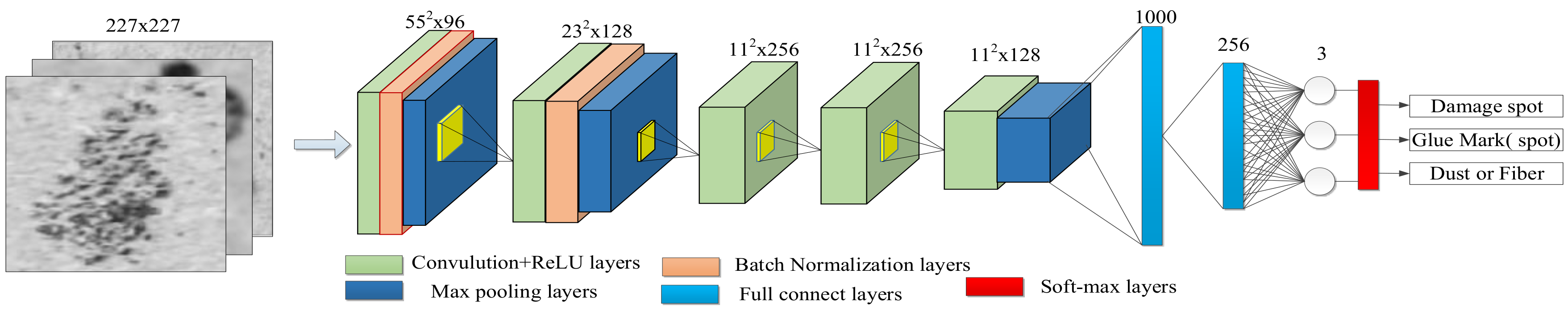
4. Classification Module

In the classification module, the defects’ regions are classified into their specific categories. When the surface film of a metallic component is different, the same defect (damage spot) may have a different color by imaging. So, the color information does not help in the classification of defects. The image’s patch of defect regions is firstly converted to gray images in order to reduce the influence of different background colors and lighting. Figure 5 shows the overall architecture of the proposed CNN. All of the grayscale images of the defect regions are resized to 227 × 227 for unified input. The proposed CNN contains five convolutional layers and three max pooling layers. The kernel size, the number of kernels, the stride, and the padding for each layer are specified in

Table 2. Structural configuration of the compact CNN.

Layers	Kernel Size	Stride	Padding	Output Size
Input	-	-	-	227 × 227
Cov1	11 × 11	4	0	55 × 55 × 96
Pool1	3 × 3	2	0	27 × 27 × 96
Cov2	5 × 5	1	0	23 × 23 × 128
Pool2	3 × 3	2	0	11 × 11 × 128
Cov3-1	3 × 3	1	1	11 × 11 × 256
Cov3-2	3 × 3	1	1	11 × 11 × 256
Cov3-3	3 × 3	1	1	11 × 11 × 128
Pool3	3 × 3	2	0	5 × 5 × 128
FC1	1000	-	-	-
FC2	256	-	-	-

. Each convolution layer is followed by a rectified linear unit (ReLU). Moreover, a batch normalization layer is added after the first two convolutional layers for speeding up the training process. It can trim the data in each channel with zero mean and unit variance. In the last layers, all of the units are fully connected to output probabilities for three classes using the softmax function.

Our proposed CNN is a compact network that is smaller than the classic classification networks such as GoogleNet [41] and ResNet [42]. This network is more suitable for the metal surface defect inspection tasks for the following two reasons. One the one hand, classical classification networks usually aim at natural images in public datasets, and their training samples far exceed the defect data in industrial inspection. Therefore, our network should be trained from scratch based on industrial defect data, instead of using the classical classification network as a pre-training model. On the other hand, the compact structure of this network reduces the classification time, and is suitable for industrial online inspection.

5. Experiments

In this section, we evaluate our method using real defect images of a metallic component. A brief description of the dataset and the experimental configuration is first provided. Then, the segmentation results as well as the classification results with comparing methods are presented in both visual and quantitative comparisons. Finally, extensive experiments for other application are reported.

5.1. Experimental Setup

Dataset Description: The dataset of metallic defect images is provided from a production line of a flat metal component using an industrial microscope. All of the components are inspected by an expert examiner in advance, and labeled with the defective region and its category. In an actual industrial production line, the number of defect images is extremely small. Moreover, a large amount of cost and manual work is required to acquire and label defect images. Finally, we collected a total of 50 images as the defect dataset, 30 of which were randomly selected as training sets, and the remaining images were used as test sets. For the segmentation task, all of the samples had their own label image. The label image was a binary image that has the same size as the original image. As shown in Figure 3, the gray value of the black pixel in the label image was 0, which represented the defect region, and the gray value of the white pixel was 255, which represented the background. However, the small size of the dataset was not enough to train a deep learning network. In order to train a suitable network, some data augmentation strategies were introduced, mainly including random rotation, translation, zoom, shear, and elastic transformation [43]. The above operations significantly increased the size of training sets, bringing the number of training sets up to 3000. For the classification task, all of the defect images were cropped out of the original images. The classification dataset contained 432 images, which included damage spots, glue marks, dust, and fibers. In the classification task, 70% of these images were used for training and 30% were used for testing.

Implementation Details: The inspection experiment system was developed using Python 3.6.2, and its deep learning computing platforms used TensorFlow [44]. The following results were obtained by a server whose CPU was Intel Core i7 and graphic processing unit (GPU) was NVIDIA GTX-1080ti with 11 GB of video memory. Aiming at training CASAE, the first AE network was trained for 30 epochs with a learning rate of 0.0001. The second network was trained for 20 epochs with the same learning rate. The batch size for both AE networks was 2. For the training of the compact CNN, we initialized the weight of each layer using a Gaussian distribution with a zero mean and a standard deviation of 0.001. The batch size was set to eight for a total of 30,000 iterations. The initial learning rate was set to 0.001. The momentum was 0.9 and the weight decay was 5 × 10⁻⁵. In the threshold module, we used 100 as the threshold G_s to refine the defects in our experiment.

In order to evaluate the inspection result and enable comparison with other methods, we adopted the intersection-over-union (IoU) and accuracy in order to quantitatively evaluate the performance of the two sub-tasks, respectively. For the segmentation task, IoU was defined as:

$$IoU(G_T,P_M)=\frac{Area(G_T\cap P_M)}{Area(G_T\cup P_M)}$$

(3)

where G_T is the ground truth mask and P_M is the predicted mask. Accuracy was used to quantitatively evaluate the performance of the classification task, which was calculated as follows:

$$Accuracy=\frac{T_P}{T_P+F_P}$$

(4)

where T_P (True Positive) and F_P (False Positive) indicate the number of defect regions correctly and incorrectly classified into their own categories.

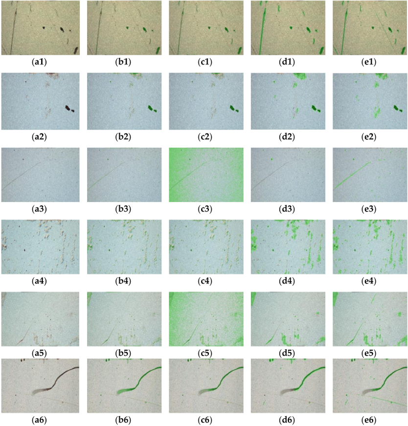
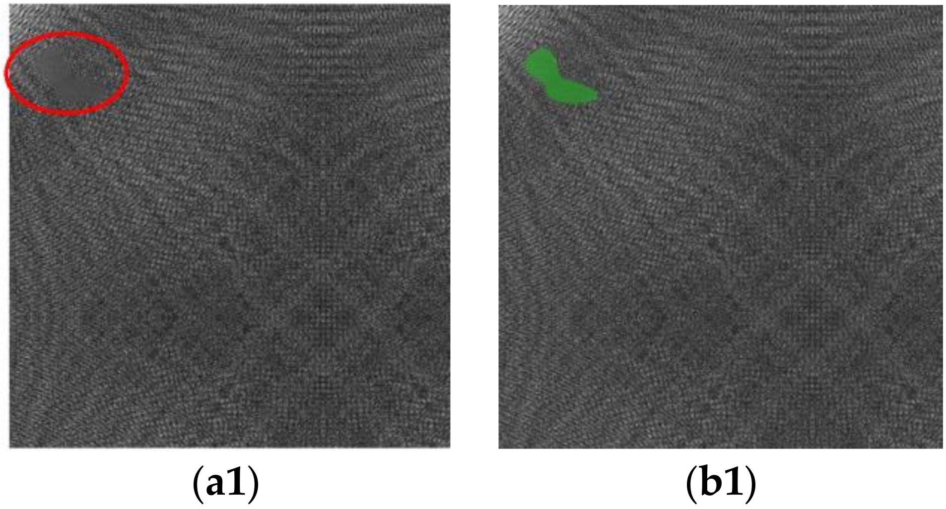
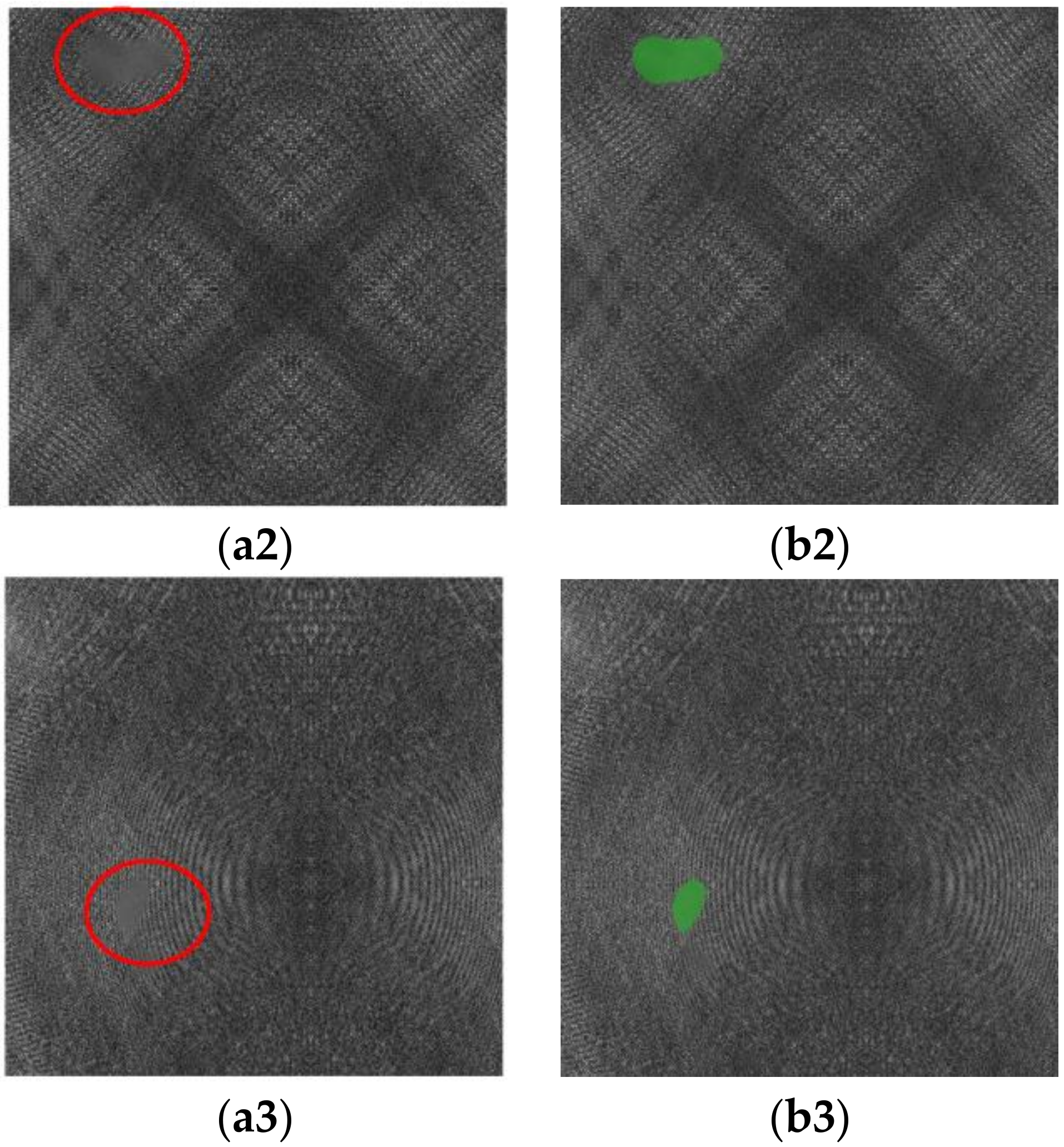
5.2. Performance of CASAE

To evaluate the performance of the CASAE on metallic defects detection, in this section, we compared the inspection performance with three detection algorithms, including the representative thresholding method [17,19] and FCN method [36]. Figure 6 shows the detection results, which are marked as a green color under various complex samples. These defective samples consist of defects with ambiguous edges (Figure 6(a2,a4,a5)), different background colors (Figure 6(a1,a6)] and low-contrast scratches (Figure 6(a3,a6)].

As can be seen from Figure 6, the thresholding methods work well only for obvious defects, e.g., the damage spots in Figure 6(a1), dust in Figure 6(a2), and fibers in Figure 6(a6). They perform poorly on ambiguous defects and low-contrast scratches, e.g., the glue spots in Figure 6(a4), scratches in Figure 6(a6). The Kittler [19] method tends to miss the detection of defects, while the Otsu [17] method easily over-detects, resulting in a large amount of background noise also being segmented, e.g., in Figure 6(c3,c5). For the FCN method [32], it can achieve good detection effects for most of the defects. However, it may be easy to ignore scratches and cannot obtain a fine defect region. In contrast to these phenomena, the proposed CASAE method provides a concise way to distinguish between defects and backgrounds. It shows powerful capabilities in various complex scenarios. The quantitative performance of defects detection results are shown in

Table 3. The quantitative performance of segmentation results with different methods.

Method	IoU
FCN [36]	81.58%
Single AE without atrous convolution	83.40%
Single AE	84.68%
CASAE without atrous convolution	87.30%
CASAE	89.60%

. As a typical segmentation network, FCN [36] is directly employed to predict the image for a starting point. As can be seen from Table 3, the AE model outperforms the FCN, which proves that the encoder–decoder structure can learn more semantic information about the defects than repeat convolution operations. Since atrous convolution is very important to produce a robust model that accommodates to the different scales of the defects, we tested its effect on the results by running the same model of a single AE and CASAE with the addition of the atrous convolution. The changes in the atrous convolution and cascaded architecture lead to an enhancement in the IoU of the testing data, as shown in the results.

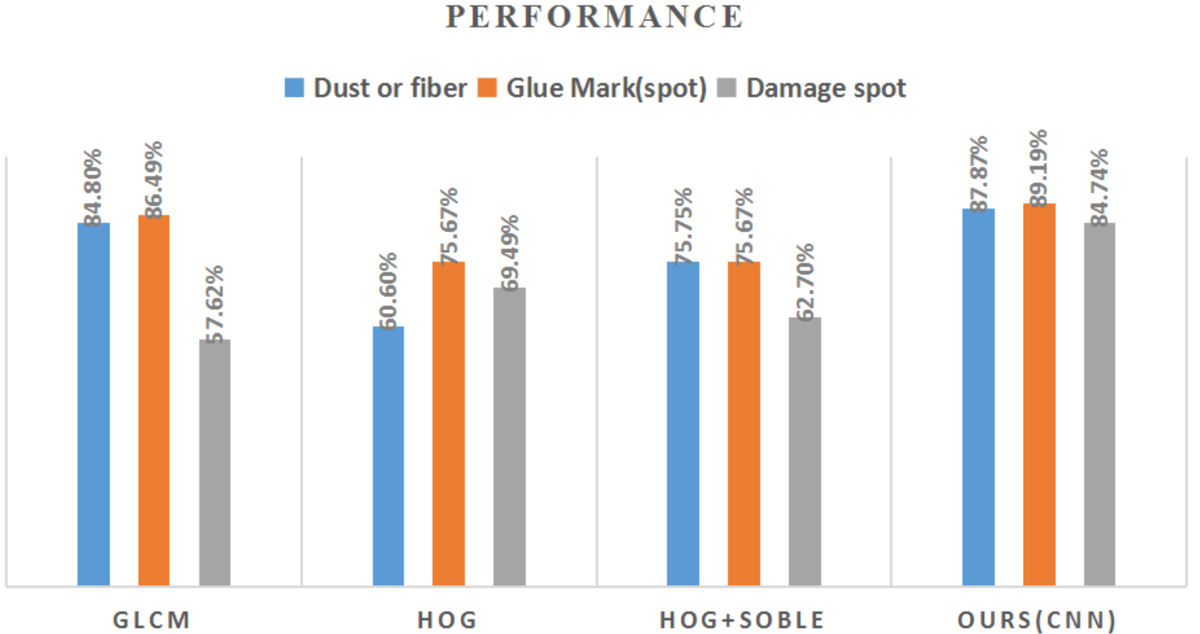
5.3. Performance of Classification Module

To evaluate the classification performance of the compact CNN quantitatively, we compared it with traditional machine learning methods with three features whose codes are publicly available. (1) GLCM [7]: this feature is the classical texture feature, which includes four typical descriptions: energy, contrast, entropy, and correlation. (2) HOG [25]: This is a directional histogram feature that is usually obtained from the following steps. Firstly, cell units are obtained by dividing the image into small, connected areas. A gradient or edge direction histogram of each pixel in the cell unit is then acquired. Finally, the complete feature descriptors are constituted by combining these histograms. (3) HOG + SOBEL: We calculate the gradient amplitude based on the SOBEL operation as a feature and combine the above HOG feature to form a new feature.

Depending on the above-mentioned features, three defect classification experiments are performed using the multi-layer perceptron (MLP). The MLP consists of 15 units in a hidden layer and an output layer with three output variables. The number of input layers is determined by the dimensions of the above features. The maximum number of iterations of the optimization algorithm in MLP is 1000. The GLCM feature consists of six gray levels to be distinguished and with a 90° direction to be calculated in the co-occurrence matrix. The quantization of the gray values in HOG is eight. The size of the filter mask in SOBEL is 3 × 3.

Table 4. The performance of classification results with different methods.

Method	Accuracy
GLCM + MLP [7]	72.86%
HOG + MLP [25]	68.99%
HOG + SOBEL + MLP	69.76%
Compact CNN	86.82%

shows the experiments results. It can be shown that the shallow feature methods based on machine learning can only achieve an accuracy of about 70%, while CNN surpasses these methods by more than 15% accuracy. The combined shallow features have a slight improvement over the single features.

Figure 7 shows the detailed classification results of the four methods. Conventional machine learning methods usually need to design features to train the model. However, CNN has achieved end-to-end training, from the feature learning to the direct output of the classification results. As shown in Figure 7, the traditional method is difficult to distinguish between the two types of dust and damage spots. This may be because both their texture and gradient information are so close that it is sometimes difficult to distinguish them from each other. However, our method can better distinguish between damage spots and dust, and the classification accuracy of the damage spots can reach more than 84%. This is explained by the existence of defects being very complex in the industrial scenarios. It is difficult to fully represent the features of actual defects only by texture and gradient features.

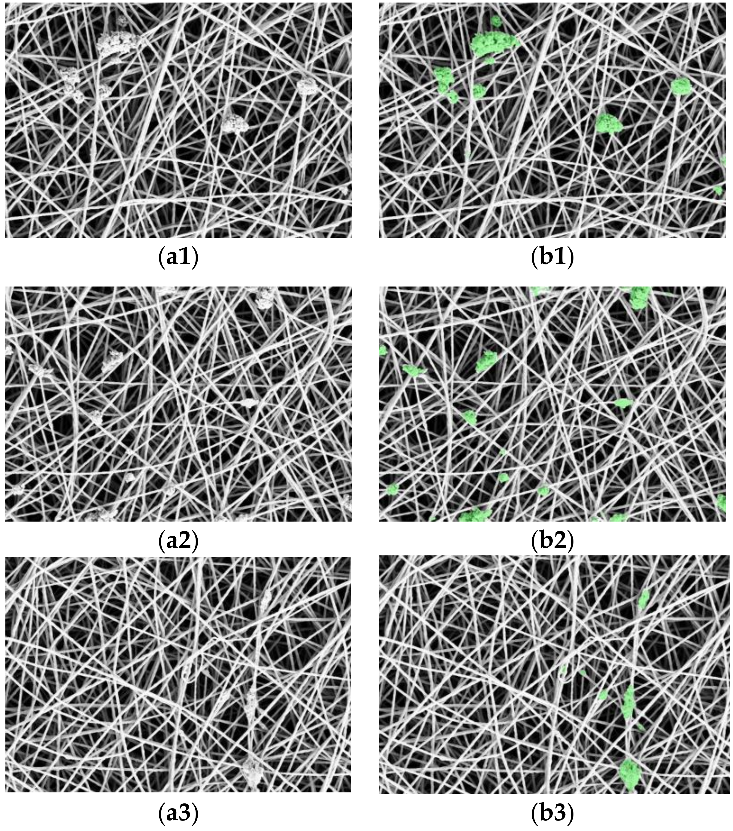
5.4. Effect of Other Application

As shown in Figure 6 and Table 3, the CASAE network can be used for metallic surface defect detection with simple training. It helps prevent the clumsy and time-consuming selection of feature and threshold parameters, and reduces the influence of different lighting and surface colours on defect detection. This detection method can also be extended to the defect inspection application that is shown in Figure 8. These images come from a public defect detection dataset [45], which consists of scanning electron microscopes (SEM) images depicting nanofibrous material produced by electrospinning.

As can be seen from Figure 8, these defects are hidden in more complex backgrounds, and the general detection methods are very difficult to detect. We use only 10 original images with data augmentation to train the CASAE model to avoid the process of extracting features from the defective block in Carrera et al. [46]. Spot defects under a random background are successfully detected using our proposed structure. It can prove that our generic algorithm can implement the production of nanofibers in order to ensure its quality.

We also test our CASAE framework on the dataset of DAGM 2007 [47], which representing defects under a textured background. The examples in Figure 9(b1–b3) show the results of the detected defects, which are marked in green on the original images. Figure 9(a1–a3) show the original images, where the defect regions are marked in red. The detailed results proved that our AE network also has a strong detection capability on defective images with textured backgrounds.

6. Conclusions

In this paper, a novel CNN-based architecture is presented to accurately perform both defect detection and classification tasks for a metallic surface against complex industrial scenarios. Defect inspection is converted to the segmentation and classification problem based on the proposed method. The proposed CASAE module can transform a defect image to a pixel-wise prediction mask that contains only defective pixels and background pixels. To quickly obtain the defect category in real inspection environments, a compact CNN is presented. The IoU score of the inspection result of our method is 89.60% using the industrial dataset. The visual and quantitative experimental results have shown that our detection algorithm is sufficient to meet the requirements of the complex industrial environment. Moreover, this generic method can be directly applied to the defect detection of other materials in industrial applications without much modification.

One limitation of the proposed method is that the training of a deep network requires manually labeled data, which takes a lot of time and expense. In the future, our ongoing work will include reducing the labeling of data with semi-supervised learning, and the application of the proposed method to more real-world inspection problems such as the inspection of mobile phone screens.

References

1. Kim, S.; Kim, W.; Noh, Y.K.; Park, F.C. Transfer learning for automated optical inspection. In Proceedings of the International Joint Conference on Neural Networks, Anchorage, AK, USA, 14–19 May 2017. [Google Scholar]
2. Song, K.; Yan, Y. A noise robust method based on completed local binary patterns for hot-rolled steel strip surface defects. Appl. Surf. Sci. 2013, 285, 858–864. [Google Scholar] [CrossRef]
3. Wu, Y.; Qin, Y.; Wang, Z.; Jia, L. A UAV-based visual inspection method for rail surface defects. Appl. Sci. 2018, 8, 1028. [Google Scholar] [CrossRef]
4. Cen, Y.G.; Zhao, R.Z.; Cen, L.H.; Cui, L.H.; Miao, Z.J.; Wei, Z. Defect inspection for TFT-LCD images based on the low-rank matrix reconstruction. Neurocomputing 2015, 149, 1206–1215. [Google Scholar] [CrossRef]
5. Lei, J.; Gao, X.; Feng, Z.; Qiu, H.; Song, M. Scale insensitive and focus driven mobile screen defect detection in industry. Neurocomputing 2018, 294, 72–81. [Google Scholar] [CrossRef]
6. Li, Y.; Zhao, W.; Pan, J. Deformable patterned fabric defect detection with Fisher criterion-based deep learning. IEEE Trans. Autom. Sci. Eng. 2017, 14, 1256–1264. [Google Scholar] [CrossRef]
7. Chondronasios, A.; Popov, I.; Jordanov, I. Feature selection for surface defect classification of extruded aluminum profiles. Int. J. Adv. Manuf. Technol. 2016, 83, 33–41. [Google Scholar] [CrossRef]
8. Gibert, X.; Patel, V.M.; Chellappa, R. Deep multitask learning for railway track inspection. IEEE Trans. Intell. Transp. Syst. 2017, 18, 153–164. [Google Scholar] [CrossRef]
9. De Araújo, S.A.; Pessota, J.H.; Kim, H.Y. Beans quality inspection using correlation-based granulometry. Eng. Appl. Artif. Intell. 2015, 40, 84–94. [Google Scholar] [CrossRef]
10. Tao, X.; Xu, D.; Zhang, Z.T.; Zhang, F.; Liu, X.L.; Zhang, D.P. Weak scratch detection and defect classification methods for a large-aperture optical element. Opt. Commun. 2017, 387, 390–400. [Google Scholar] [CrossRef]
11. Ren, R.; Hung, T.; Tan, K.C. A generic deep-learning-based approach for automated surface inspection. IEEE Trans. Cybern. 2018, 48, 929–940. [Google Scholar] [PubMed]
12. Tsanakas, J.A.; Chrysostomou, D.; Botsaris, P.N.; Gasteratos, A. Fault diagnosis of photovoltaic modules through image processing and Canny edge detection on field thermographic measurements. Int. J. Sustain. Energy 2015, 34, 351–372. [Google Scholar] [CrossRef]
13. Tastimur, C.; Yetis, H.; Karaköse, M.; Akin, E. Rail defect detection and classification with real time image processing technique. Int. J. Comput. Sci. Softw. Eng. 2016, 5, 283. [Google Scholar]
14. Jian, C.; Gao, J.; Ao, Y. Automatic surface defect detection for mobile phone screen glass based on machine vision. Appl. Soft Comput. 2017, 52, 348–358. [Google Scholar] [CrossRef]
15. Mak, K.L.; Peng, P.; Yiu, K.F. Fabric defect detection using morphological filters. Image Vis. Comput. 2009, 27, 1585–1592. [Google Scholar] [CrossRef]
16. Li, X.; Gao, B.; Woo, W.L.; Tian, G.Y.; Qiu, X.; Gu, L. Quantitative surface crack evaluation based on eddy current pulsed thermography. IEEE Sens. J. 2017, 17, 412–421. [Google Scholar] [CrossRef]
17. Yuan, X.; Wu, L.; Peng, Q. An improved Otsu method using the weighted object variance for defect detection. Appl. Surf. Sci. 2015, 349, 472–484. [Google Scholar] [CrossRef] [Green Version]
18. Win, M.; Bushroa, A.R.; Hassan, M.A.; Hilman, N.M.; Ide-Ektessabi, A. A contrast adjustment thresholding method for surface defect detection based on mesoscopy. IEEE Trans. Ind. Inform. 2015, 11, 642–649. [Google Scholar] [CrossRef]
19. Kalaiselvi, T.; Nagaraja, P. A rapid automatic brain tumor detection method for MRI images using modified minimum error thresholding technique. Int. J. Imaging Syst. Technol. 2015, 1, 77–85. [Google Scholar]
20. Wang, L.; Zhao, Y.; Zhou, Y.; Hao, J. Calculation of flexible printed circuit boards (FPC) global and local defect detection based on computer vision. Circ. World 2016, 42, 49–54. [Google Scholar] [CrossRef]
21. Bai, X.; Fang, Y.; Lin, W.; Wang, L.; Ju, B.F. Saliency-based defect detection in industrial images by using phase spectrum. IEEE Trans. Ind. Inform. 2014, 10, 2135–2145. [Google Scholar] [CrossRef]
22. Borwankar, R.; Ludwig, R. An Optical Surface Inspection and Automatic Classification Technique Using the Rotated Wavelet Transform. IEEE Trans. Instrum. Meas. 2018, 67, 690–697. [Google Scholar] [CrossRef]
23. Hu, G.H. Automated defect detection in textured surfaces using optimal elliptical Gabor filters. Optik 2015, 126, 1331–1340. [Google Scholar] [CrossRef]
24. Susan, S.; Sharma, M. Automatic texture defect detection using Gaussian mixture entropy modeling. Neurocomputing 2017, 239, 232–237. [Google Scholar] [CrossRef]
25. Shumin, D.; Zhoufeng, L.; Chunlei, L. Adaboost learning for fabric defect detection based on hog and SVM. In Proceedings of the International Conference on Multimedia Technology, Hangzhou, China, 26–28 July 2011. [Google Scholar]
26. Jia, F.; Lei, Y.; Lu, N.; Xing, S. Deep normalized convolutional neural network for imbalanced fault classification of machinery and its understanding via visualization. Mech. Syst. Signal Process. 2018, 110, 349–367. [Google Scholar] [CrossRef]
27. Glowacz, A. Acoustic based fault diagnosis of three-phase induction motor. Appl. Acoust. 2018, 137, 82–89. [Google Scholar] [CrossRef]
28. Tadeusiewicz, R. Neural networks in mining sciences—General overview and some representative examples. Arch. Min. Sci. 2015, 60, 971–984. [Google Scholar] [CrossRef]
29. Ganovska, B.; Molitoris, M.; Hosovsky, A.; Pitel, J.; Krolczyk, J.B.; Ruggierio, A.; Krolczyk, G.M.; Hloch, S. Design of the model for the on-line control of the AWJ technology based on neural networks. Indian J. Eng. Mater. Sci. 2016, 23, 279–287. [Google Scholar]
30. Masci, J.; Meier, U.; Fricout, G.; Schmidhuber, J. Multi-scale pyramidal pooling network for generic steel defect classification. In Proceedings of the International Joint Conference on Neural Networks, Dallas, TX, USA, 4–9 August 2013. [Google Scholar]
31. Natarajan, V.; Hung, T.Y.; Vaikundam, S.; Chia, L.T. Convolutional networks for voting-based anomaly classification in metal surface inspection. In Proceedings of the IEEE International Conference on Industrial Technology, Toronto, ON, Canada, 22–25 March 2017. [Google Scholar]
32. Wang, T.; Chen, Y.; Qiao, M.; Snoussi, H. A fast and robust convolutional neural network-based defect detection model in product quality control. Int. J. Adv. Manuf. Technol. 2018, 94, 3465–3471. [Google Scholar] [CrossRef]
33. Cha, Y.J.; Choi, W.; Suh, G.; Mahmoudkhani, S.; Büyüköztürk, O. Autonomous structural visual inspection using region—Based deep learning for detecting multiple damage types. Comput.-Aided Civ. Infrastruct. Eng. 2018, 33, 731–747. [Google Scholar] [CrossRef]
34. Lin, H.; Li, B.; Wang, X.; Shu, Y.; Niu, S. Automated defect inspection of LED chip using deep convolutional neural network. J. Intell. Manuf. 2018, 29, 1–10. [Google Scholar] [CrossRef]
35. Chen, J.; Liu, Z.; Wang, H.; Núñez, A.; Han, Z. Automatic defect detection of fasteners on the catenary support device using deep convolutional neural network. IEEE Trans. Instrum. Meas. 2018, 67, 257–269. [Google Scholar] [CrossRef]
36. Xiao, Z.; Leng, Y.; Geng, L.; Xi, J. Defect detection and classification of galvanized stamping parts based on fully convolution neural network. In Proceedings of the Ninth International Conference on Graphic and Image Processing (ICGIP 2017), Qingdao, China, 14–16 October 2017. [Google Scholar]
37. Liu, W.; Wang, Z.; Liu, X.; Zeng, N.; Liu, Y.; Alsaadi, F.E. A survey of deep neural network architectures and their applications. Neurocomputing 2017, 234, 11–26. [Google Scholar] [CrossRef]
38. Karen, S.; Andrew, Z. Very deep convolutional networks for large-scale image recognition. In Proceedings of the International Conference On Representation Learning (ICRL 2015), San Diego, CA, USA, 7–9 May 2015. [Google Scholar]
39. Islam, M.A.; Rochan, M.; Bruce, N.D.; Wang, Y. Gated feedback refinement network for dense image labeling. In Proceedings of the IEEE Conference on Computer Vision and Pattern Recognition (CVPR), Honolulu, HI, USA, 21–26 July 2017. [Google Scholar]
40. Chen, L.C.; Papandreou, G.; Schroff, F.; Adam, H. Rethinking Atrous Convolution for Semantic Image Segmentation. Available online: https://pdfs.semanticscholar.org/efb3/fec61a1433609635f2bd21a18f8b6ef47541.pdf (accessed on 20 August 2018).
41. Szegedy, C.; Liu, W.; Jia, Y.; Sermanet, P.; Reed, S.; Anguelov, D.; Erhan, D.; Vanhoucke, V.; Rabinovich, A. Going deeper with convolutions. In Proceedings of the IEEE Conference on Computer Vision and Pattern Recognition, Boston, MA, USA, 8–10 June 2015. [Google Scholar]
42. He, K.; Zhang, X.; Ren, S.; Sun, J. Deep residual learning for image recognition. In Proceedings of the IEEE Conference on Computer Vision and Pattern Recognition, Las Vegas, NV, USA, 26 June–1 July 2016. [Google Scholar]
43. Schaefer, S.; McPhail, T.; Warren, J. Image deformation using moving least squares. ACM Trans. Gr. (TOG) 2006, 25, 533–540. [Google Scholar] [CrossRef]
44. Abadi, M.; Barham, P.; Chen, J.; Chen, Z.; Davis, A.; Dean, J.; Devin, M.; Ghemawat, S.; Irving, G.; Isard, M.; et al. TensorFlow: A system for large-scale machine learning. OSDI 2016, 16, 265–283. [Google Scholar]
45. Consiglio Nazionale Delle Ricerche. Matlab Tool for Analyzing SEM Images of Electrospun Material. Available online: http://www.mi.imati.cnr.it/ettore/NanoTWICE/ (accessed on 3 December 2017).
46. Carrera, D.; Manganini, F.; Boracchi, G.; Lanzarone, E. Defect detection in SEM images of nanofibrous materials. IEEE Trans. Ind. Inform. 2017, 13, 551–561. [Google Scholar] [CrossRef]
47. DAGM 2007 Datasets. Available online: https://hci.iwr.uni-heidelberg.de/node/3616 (accessed on 27 February 2018).
Figure 1. Challenges of detecting surface defects of metallic components. (a) Defects with various shapes and sizes, (b1) defects with ambiguous edges and low contrast, (b2) defects with different background, (b3) fiber, (b4) dust, (b5,b6) scratches.
Applsci 08 01575 g001
Figure 2. The pipeline of the proposed metallic surface defect inspection architecture. (a) Original image, (b) defect segment, (c) defect location, (d) cropped results, and (e) classification.
Applsci 08 01575 g002
Figure 3. The architecture of the autoencoder (AE) network.
Applsci 08 01575 g003
Figure 4. Illustration of atrous convolution.
Applsci 08 01575 g004
Figure 5. The architecture of a compact convolutional neural network (CNN).
Applsci 08 01575 g005
Figure 6. Segmentation results. The six rows are examples of defective images. (a1a6) raw images, (b1b6) results of Kittler [19], (c1c6) results of Otsu [17], (d1d6) results of a fully convolutional network (FCN) [36], (e1e6) results of the cascaded autoencoder (CASAE) (proposed).
Applsci 08 01575 g006
Figure 7. Detail classification results of four methods.
Applsci 08 01575 g007
Figure 8. Examples of CASAE-processed images for different applications. The first columns are examples of (a1a3) SEM images, and (b1b3) result images of spot defects are marked in green.
Applsci 08 01575 g008
Figure 9. Examples of CASAE-processed images with textured backgrounds. The first columns are examples of (a1a3) defects images and (b1b3) result images of defects marked in green.
Applsci 08 01575 g009aApplsci 08 01575 g009b