Article

Global Dynamics of Modeling Flocculation of Microorganism

1
Department of Applied Mathematics, School of Mathematics and Physics, University of Science and Technology Beijing, Beijing 100083, China
2
Department of Biological Science and Technology, School of Chemical and Biological Engineering, University of Science and Technology Beijing, Beijing 100083, China
*
Author to whom correspondence should be addressed.
Appl. Sci. 2016, 6(8), 221; https://doi.org/10.3390/app6080221
Submission received: 31 May 2016 / Accepted: 26 July 2016 / Published: 5 August 2016
(This article belongs to the Special Issue Dynamical Models of Biology and Medicine)

Abstract

:
From a biological perspective, a dynamic model describing the cultivation and flocculation of a microorganism that uses two different kinds of nutrients (carbon source and nitrogen source) is proposed. For the proposed model, there always exists a boundary equilibrium, i.e., R h o d o p s e u d o m o n a s p a l u s t r i s -free equilibrium. Furthermore, under additional conditions, the model also has five positive equilibria at most, i.e., the equilibria for which carbon source, nitrogen source, R h o d o p s e u d o m o n a s p a l u s t r i s and flocculants are coexistent. The phenomena of backward and forward bifurcations are extensively discussed by using center manifold theory. The global stability of the boundary equilibrium of the proposed model is deeply investigated. Moreover, the local stability of the positive equilibrium and the uniform persistence of the proposed model are discussed. Under additional conditions, the global stability of the positive equilibrium is studied. Some control strategies are given by the theoretical analysis. Finally, some numerical simulations are performed to confirm the correctness of the theoretical results.

Graphical Abstract

1. Introduction

Photosynthetic bacteria, which are common microorganisms in the natural environment, have been applied in the field of environmental protection, such as in the treatment of sewage, domestic wastewater and the bioremediation of sediment mud polluted with organic matter (see, for example, [1,2,3,4]). On the other hand, photosynthetic bacteria can produce relatively large amounts of physiologically-active substances, such as vitamin B 12 , ubiquinone (coenzyme Q 10 ), 5-aminolevulinic acid (ALA) and RNA (see, for example [5]). In particular, vitamin B 12 has been used in treating anemia and as an eye lotion. Recently, applications as health food supplements have received considerable attention. Coenzyme Q 10 has been used in treating heart diseases for many years. Further, coenzyme Q 10 has been used not only as a medicine, but also as some food supplements, because of its physiological activities. One of the developments of ALA applications is in the area of photodynamic diagnosis. RNA is an attractive source of 5 -ribonucleotides for use as a flavor enhancer in the food industry. In recent years, the production of RNA has been used as a dietary source of pyrimidine for human immune functions (see, for example [6,7]).
Some photosynthetic bacteria, such as R h o d o p s e u d o m o n a s p a l u s t r i s , are extensively used in the production of lycopene, aquaculture, and so on [8]. It can use sunlight, inorganic and organic compounds for energy. Further, R h o d o p s e u d o m o n a s p a l u s t r i s can have practical value for removing microcystin from the water body during algal blooms [9]. It can also degrade 2,4,6-trinitrotoluene (TNT), which has negative effects on the human body and aquatic life, resulting in a major threat to drinking and irrigation water supplies, as well as the recreational use of surface waters worldwide. Moreover, R h o d o p s e u d o m o n a s p a l u s t r i s is regarded as the most promising microbial system for the biological production of hydrogen, which has been extensively developed because of its high-energy content and clean product after combustion [10]. However, the concentration of R h o d o p s e u d o m o n a s p a l u s t r i s is very low under anaerobic light culture conditions (see, for example, [11,12]). Therefore, cost-efficient harvesting of R h o d o p s e u d o m o n a s p a l u s t r i s is a new challenge. In order to harvest R h o d o p s e u d o m o n a s p a l u s t r i s from the liquid, it is necessary to flocculate the single cells into large cell aggregates. Flocculation is a chemically-based separation process that requires less energy than centrifugation and ultrafiltration and, thus, is regarded as the most promising means for degrading microorganisms. Since algal toxins of blooms have happened occasionally in recent years, the problems of degrading microorganisms have received wide attentions (see, for example, [13,14,15,16]).
Flocculants are a kind of important water treatment reagent, which can be divided into organic flocculants and inorganic flocculants according to the chemical compositions [17]. Although organic flocculants, such as polyacrylamide, are frequently used in wastewater treatment and industrial downstream processes because of their high efficiency, some of them are not easily degraded in nature [18,19], and some of the monomers derived from synthetic polymers are harmful to the human body (see, for example, [20,21]). To solve these environmental problems, inorganic flocculants are increasingly being seen as an alternative in the settlement of microorganisms, more specifically in wastewater treatment owing to their inexpensive and nontoxic characteristics. Thus, inorganic flocculants may be used as nontoxic, cost-effective and widely-available flocculants for harvesting R h o d o p s e u d o m o n a s p a l u s t r i s (see, for example, [22,23,24,25,26,27] and the references therein).
Mathematical models have played an important role in better understanding microbiology and population biology (see, for example, [28,29]). In recent years, the dynamics of the chemostat models has received considerable attentions (see, for example, [29]). The article of Smith and Waltman has played an important role in the development of the chemostat models [30]. From then on, much research on the chemostat models has been extensively studied by many authors. A model describing two populations of microorganisms competing for one single limiting nutrients was proposed in [31]. Later, the model was extended to an arbitrary number of populations in [32,33]. These models, which were studied in articles [31,32,33], have proven that they all include a competitive exclusion effect. In the articles [34,35,36,37,38,39], some further developments have been performed on the chemostat models to place the relevant models in a naturally more sensible manner.
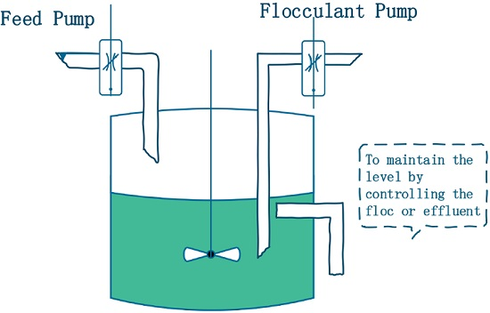
Let S ( t ) and X ( t ) denote the concentration of the nutrients and R h o d o p s e u d o m o n a s p a l u s t r i s , respectively, in the culture vessel at time t. P ( t ) denotes the concentration of inorganic flocculants, which are used for harvesting R h o d o p s e u d o m o n a s p a l u s t r i s (see Figure 1). The constants S 0 > 0 and P 0 > 0 denote the input concentration of the nutrients and flocculants, respectively. For simplicity, it is assumed that the input of the nutrients and flocculants is continuous. The constant D > 0 is the dilution rate of the chemostat.
The constant τ 0 denotes the time delay involved in the conversion of nutrients to R h o d o p s e u d o m o n a s p a l u s t r i s . The flocculation rate of microorganisms is assumed to be a bilinear mass-action function response m 1 X ( t ) P ( t ) , where m 1 0 is the per capita contact rate. At the same time, flocculants produce loss or consumption [17], and the loss rate of flocculants is also assumed to be a bilinear mass-action function response m 2 X ( t ) P ( t ) , where m 2 0 is constant. Thus, in [40], the following dynamic model has been proposed:
d S ( t ) d t = ( S 0 - S ( t ) ) D - r 1 S ( t ) X ( t ) , d X ( t ) d t = r S ( t - τ ) X ( t - τ ) - D X ( t ) - m 1 X ( t ) P ( t ) , d P ( t ) d t = ( P 0 - P ( t ) ) D - m 2 X ( t ) P ( t ) .
In Model (1), r 0 and r 1 0 are constants, and the bilinear mass-action uptake function S ( t ) X ( t ) has been used.
It should be mentioned here that, the analysis reveals that Model (1) proposed in [40] exhibits the phenomenon of backward bifurcation for the existence of positive equilibria. Moreover, the local stability properties of the equilibria have been dealt with in detail.
People found that the influence of different nutrients has played an important role in the culture of microorganisms. In order to take this into consideration, appropriate combinations of nutrients are considered in chemostat models. Models with two competitors and two perfectly-complemented growth-limiting nutrients are studied in [41,42]. Local asymptotic conditions for the equilibria are derived.
When there is a microorganism to compete for two or more resources, it may become necessary to consider how the resources, once consumed, interact to promote growth. In [41], the authors employ consumer needs to provide a criterion to classify resources and classify resources as perfectly complementary, perfectly substitutable or imperfectly substitutable. Perfectly-complementary resources are different essential substances that must be taken together. In this case, each substance fulfills different functions with respect to the growth of microorganisms. For example, carbon source and nitrogen source may be complementary for the growth of bacterium.
Motivated by the papers mentioned above, in this paper, we further consider a dynamic model describing the cultivation and flocculation of R h o d o p s e u d o m o n a s p a l u s t r i s , and the nutrients presented in [40] will be divided into carbon source and nitrogen source, which are perfectly complementary in the culture of R h o d o p s e u d o m o n a s p a l u s t r i s (see, for example, [5,41,42,43,44]). We assume that the growth of R h o d o p s e u d o m o n a s p a l u s t r i s is always co-limited by carbon and nitrogen for all possible nutrient conditions. We do not consider the case where only one of these nutrients limits growth, for example, in environmental scenarios of high carbon, but very low nitrogen loads, the growth of bacteria may be purely nitrogen limited.
Let C ( t ) and N ( t ) denote the concentration of carbon source and nitrogen source, respectively, in the culture vessel at time t. The constants C 0 > 0 and N 0 > 0 denote the input concentration of carbon source and nitrogen source, respectively. We assume that the conversion of nutrients to microorganism biomass occurs instantly. That is, the time delay τ in Model (1) equals zero. Hence, we have the following dynamic model describing the cultivation and flocculation of a microorganism:
d C ( t ) d t = ( C 0 - C ( t ) ) D - X ( t ) δ 1 r 1 μ 1 ( C ( t ) ) μ 2 ( N ( t ) ) , d N ( t ) d t = ( N 0 - N ( t ) ) D - X ( t ) δ 2 r 2 μ 1 ( C ( t ) ) μ 2 ( N ( t ) ) , d X ( t ) d t = r μ 1 ( C ( t ) ) μ 2 ( N ( t ) ) X ( t ) - D X ( t ) - m 1 X ( t ) P ( t ) , d P ( t ) d t = ( P 0 - P ( t ) ) D - m 2 X ( t ) P ( t ) .
In Model (2), the parameters D, r, m 1 , m 2 and P 0 are the same as Model (1). The term r μ 1 ( C ( t ) ) μ 2 ( N ( t ) ) is the growth rate of R h o d o p s e u d o m o n a s p a l u s t r i s , and the terms r 1 μ 1 ( C ( t ) ) μ 2 ( N ( t ) ) and r 2 μ 1 ( C ( t ) ) μ 2 ( N ( t ) ) represent the quantity of the decreasing of the carbon source and nitrogen source, respectively, where r 1 and r 2 are non-negative constants; the functions μ 1 ( C ( t ) ) and μ 2 ( N ( t ) ) are nonnegative and continuous for C ( t ) 0 , N ( t ) 0 . For the simplicity of the theoretical analysis, in this paper, the functions μ 1 ( C ( t ) ) and μ 2 ( N ( t ) ) are chosen as Monod-type functions, i.e.,
μ 1 ( C ( t ) ) = C ( t ) K 1 + C ( t ) , μ 2 ( N ( t ) ) = N ( t ) K 2 + N ( t ) ,
where K 1 > 0 and K 2 > 0 are the half-saturation constants with respect to the carbon source and nitrogen source, respectively. δ i ( i = 1 , 2 ) are yield coefficients (see, for example, [29]), which are defined as:
δ i = m a s s o f o r g a n i s m f o r m e d m a s s o f s u b s t r a t e c o n s u m e d , ( i = 1 , 2 ) .
Therefore, the dynamic Model (2) can be rewritten in the following form:
d C ( t ) d t = ( C 0 - C ( t ) ) D - r 1 C ( t ) N ( t ) X ( t ) δ 1 ( K 1 + C ( t ) ) ( K 2 + N ( t ) ) , d N ( t ) d t = ( N 0 - N ( t ) ) D - r 2 C ( t ) N ( t ) X ( t ) δ 2 ( K 1 + C ( t ) ) ( K 2 + N ( t ) ) , d X ( t ) d t = r C ( t ) N ( t ) X ( t ) ( K 1 + C ( t ) ) ( K 2 + N ( t ) ) - D X ( t ) - m 1 X ( t ) P ( t ) , d P ( t ) d t = ( P 0 - P ( t ) ) D - m 2 X ( t ) P ( t ) .
It is convenient to introduce dimensionless variables. In particular, we define:
C ¯ = C C 0 , N ¯ = N N 0 , X ¯ = X , P ¯ = P P 0 , K ¯ 1 = K 1 C 0 , K ¯ 2 = K 2 N 0 , t ¯ = t D ,
r ¯ 1 = r 1 δ 1 D C 0 , r ¯ 2 = r 2 δ 2 D N 0 , r ¯ = r D , m ¯ 1 = m 1 P 0 D , m ¯ 2 = m 2 D ,
and still denote C ¯ , N ¯ , X ¯ , P ¯ , K ¯ 1 , K ¯ 2 , t ¯ , r ¯ 1 , r ¯ 2 , r ¯ , m ¯ 1 and m ¯ 2 with C , N , X , P , K 1 , K 2 , t, r 1 , r 2 , r, m 1 and m 2 , then Model (3) becomes:
d C ( t ) d t = 1 - C ( t ) - r 1 C ( t ) N ( t ) X ( t ) ( K 1 + C ( t ) ) ( K 2 + N ( t ) ) , d N ( t ) d t = 1 - N ( t ) - r 2 C ( t ) N ( t ) X ( t ) ( K 1 + C ( t ) ) ( K 2 + N ( t ) ) , d X ( t ) d t = r C ( t ) N ( t ) X ( t ) ( K 1 + C ( t ) ) ( K 2 + N ( t ) ) - X ( t ) - m 1 X ( t ) P ( t ) , d P ( t ) d t = 1 - P ( t ) - m 2 X ( t ) P ( t ) .
According to the biological considerations, the initial condition of Model (4) is given as:
C ( 0 ) = C 0 0 , N ( 0 ) = N 0 0 , X ( 0 ) = X 0 0 , P ( 0 ) = P 0 0 ,
where the constants C 0 , N 0 , X 0 and P 0 represent the initial concentration of the carbon source, nitrogen source, R h o d o p s e u d o m o n a s p a l u s t r i s and flocculants respectively.
The purpose of this paper is to tackle the existence of backward and forward bifurcations by using center manifold theory and to investigate the global stability properties of the two classes of equilibria by constructing the suitable Lyapunov functions.
The organization of the paper is as follows. The global existence, nonnegativity and boundedness of the solutions of Model (4) are investigated in Section 2. In Section 3, the existence of the equilibria and the phenomena of backward and forward bifurcations are extensively discussed. In Section 4, the global stability of the boundary equilibrium of Model (4) is discussed by the stability theory of ordinary differential equations. Furthermore, we consider the local stability of positive equilibrium, the uniform persistence of Model (4) and the global asymptotic stability of the positive equilibrium in Section 5. In Section 6, some control strategies are given by the theoretical analysis. Some discussions are given in Section 7.

2. The Global Existence, Nonnegativity and Boundedness of Solutions

From the biological considerations, it is necessary to show that all of the solutions of Model (4) are nonnegative and bounded for all t 0 . By using the basic theory of ordinary differential equations [45] and some simple calculations, it is not difficult to show the following result.
Theorem 1. 
The solution ( C ( t ) , N ( t ) , X ( t ) , P ( t ) ) of Model (4) with the initial Condition (5) is existent, unique and nonnegative for all t 0 and satisfies:
lim sup t C ( t ) 1 , lim sup t N ( t ) 1 , lim sup t M ( t ) α ,
lim sup t P ( t ) 1 , lim inf t C ( t ) C ̲ , lim inf t N ( t ) N ̲ , lim inf t P ( t ) P ̲ ,
where M ( t ) = r 2 r 1 C ( t ) + r 2 r 2 N ( t ) + X ( t ) , α = r 2 r 1 + r 2 r 2 , C ̲ = K 1 ( K 2 + 1 ) K 1 ( K 2 + 1 ) + r 1 α , N ̲ = K 2 ( K 1 + 1 ) K 2 ( K 1 + 1 ) + r 2 α , P ̲ = 1 1 + m 2 α .
Proof. 
From the theory of the local existence of solutions for ordinary differential equations, it can be obtained that the solution ( C ( t ) , N ( t ) , X ( t ) , P ( t ) ) of Model (4) is existent and unique for t [ 0 , δ ) . Here, δ is some positive constant [29,45,46]. Furthermore, we also have that the solution ( C ( t ) , N ( t ) , X ( t ) , P ( t ) ) is nonnegative for t [ 0 , δ ) .
We can easily show that C ( t ) , N ( t ) and P ( t ) are bounded on t [ 0 , δ ) . Let us further show that X ( t ) is also bounded on t [ 0 , δ ) . For t 0 , define:
M ( t ) = r 2 r 1 C ( t ) + r 2 r 2 N ( t ) + X ( t ) .
From Model (4), we obtain that, for t 0 ,
M ˙ ( t ) r 2 r 1 + r 2 r 2 - M ( t ) .
From (6) and the well-known comparison principle, we have that M ( t ) is also bounded for t [ 0 , δ ) . Hence, by employing the continuation theorems of the solutions [29,45,46], the solution ( C ( t ) , N ( t ) , X ( t ) , P ( t ) ) is existent and unique for any t 0 . Similarly, the solution is nonnegative for any t 0 .
Thus, from the comparison principle, we have that:
lim sup t C ( t ) 1 , lim sup t N ( t ) 1 , lim sup t M ( t ) r 2 r 1 + r 2 r 2 = α , lim sup t P ( t ) 1 .
By the first equation of Model (4), we obtain that, for t 0 ,
C ˙ ( t ) = 1 - C ( t ) - r 1 C ( t ) N ( t ) X ( t ) ( K 1 + C ( t ) ) ( K 2 + N ( t ) ) 1 - 1 + r 1 α K 1 ( K 2 + 1 ) C ( t ) .
Again, we can conclude that lim inf t C ( t ) C ̲ . By using the technique similar above, we can show that lim inf t N ( t ) N ̲ , lim inf t P ( t ) P ̲ . We complete the proof of Theorem 1. □
Theorem 2. 
The compact set:
Ω = { ( C , N , X , P ) R + 4 | C ̲ C 1 , N ̲ N 1 , 0 M α , P ̲ P 1 }
attracts all of the solutions of Model (4) and is positively invariant with respect to Model (4).
Proof. 
According to Theorem 1, it only needs to be proven that Ω is positively invariant with respect to Model (4). That is, it needs to be shown that C ̲ C ( t ) 1 , N ̲ N ( t ) 1 , M ( t ) α , P ̲ P ( t ) 1 for any t 0 if ( C ( 0 ) , N ( 0 ) , X ( 0 ) , P ( 0 ) ) Ω . Let us show M ( t ) α for any t 0 .
In fact, if there exists some t 1 > 0 , such that M ( t 1 ) > α , then t 1 * = sup { t | M ( t ) = α , t [ 0 , t 1 ] } is existent and t 1 * 0 . Hence, we obtain that M ( t 1 * ) = α , M ( t 1 ) > α and M ( t ) > α for t ( t 1 * , t 1 ) . By the Lagrange mean-value theorem, there exists some t 2 ( t 1 * , t 1 ) , such that M ˙ ( t 2 ) = M ( t 1 ) - M ( t 1 * ) t 1 - t 1 * > 0 .
On the other hand, from (6), we have that M ˙ ( t 2 ) α - M ( t 2 ) < α - α = 0 , which is a contradiction. Thus, M ( t ) α for any t 0 . Therefore, from Model (4), we have that for any t 0 , C ˙ ( t ) 1 - C ( t ) , N ˙ ( t ) 1 - N ( t ) , P ˙ ( t ) 1 - P ( t ) , from which we easily have that C ( t ) 1 , N ( t ) 1 , P ( t ) 1 for any t 0 .
Next, we prove that C C ̲ for any t 0 if ( C ( 0 ) , N ( 0 ) , X ( 0 ) , P ( 0 ) ) Ω .
In fact, if there exists some t 3 > 0 , such that C ( t 3 ) < C ̲ , then t 2 * = sup { t | C ( t ) = C ̲ , t [ 0 , t 3 ] } is existent and t 2 * 0 . Hence, we have that C ( t 2 * ) = C ̲ , C ( t 3 ) < C ̲ and C ( t ) < C ̲ for t ( t 2 * , t 3 ) . By the Lagrange mean-value theorem, there exists some t 4 ( t 2 * , t 3 ) , such that C ˙ ( t 4 ) = C ( t 3 ) - C ( t 2 * ) t 3 - t 2 * < 0 .
On the other hand, from Model (4), we obtain that:
C ˙ ( t 4 ) 1 - C ( t 4 ) - r 1 C ( t 4 ) α K 1 ( K 2 + 1 ) > 1 - 1 + r 1 α K 1 ( K 2 + 1 ) C ̲ = 0 ,
which is a contradiction. Thus, C ( t ) C ̲ for any t 0 . Therefore, from Model (4), we obtain that, for any t 0 ,
N ˙ ( t ) 1 - 1 + r 2 α K 2 ( K 1 + 1 ) N ( t ) , P ˙ ( t ) 1 - ( 1 + m 2 α ) P ( t ) ,
from which we easily obtain that N ̲ N ( t ) , P ̲ P ( t ) , for any t 0 . This completes the proof of Theorem 2. □

3. The Existence of the Equilibria and Its Classification

Let ( C , N , X , P ) be any equilibrium of Model (4). Then, ( C , N , X , P ) satisfies the following nonlinear algebraic equations,
1 - C - r 1 C N X ( K 1 + C ) ( K 2 + N ) = 0 , 1 - N - r 2 C N X ( K 1 + C ) ( K 2 + N ) = 0 , r C N X ( K 1 + C ) ( K 2 + N ) - X - m 1 X P = 0 , 1 - P - m 2 X P = 0 .
Model (4) always has the boundary equilibrium E 0 ( 1 , 1 , 0 , 1 ) . The existence of E 0 indicates that, if there is no R h o d o p s e u d o m o n a s p a l u s t r i s to be added into the culture vessel at the beginning of the culture, the concentrations of the carbon source, nitrogen source and flocculants always maintain the constant values 1, 1 and 1, respectively. The equilibrium E 0 ( 1 , 1 , 0 , 1 ) is also called R h o d o p s e u d o m o n a s p a l u s t r i s -free equilibrium.
Define the basic bifurcation parameter as:
R 0 = r ( K 1 + 1 ) ( K 2 + 1 ) ( m 1 + 1 ) .
Let ( C * , N * , X * , P * ) be any positive equilibrium of Model (4). From (7), we have that:
( K 1 + C * ) ( K 2 + N * ) ( 1 + m 1 1 + m 2 X * ) - r C * N * = 0 , P * = 1 1 + m 2 X * , C * = - r 1 m 2 ( X * ) 2 + ( m 2 r - r 1 ( m 1 + 1 ) ) X * + r r ( 1 + m 2 X * ) , N * = - r 2 m 2 ( X * ) 2 + ( m 2 r - r 2 ( m 1 + 1 ) ) X * + r r ( 1 + m 2 X * ) .
Clearly, X * should satisfy the following conditions:
- r 1 m 2 ( X * ) 2 + m 2 r - r 1 ( m 1 + 1 ) X * + r > 0 , - r 2 m 2 ( X * ) 2 + m 2 r - r 2 ( m 1 + 1 ) X * + r > 0 .
Substituting the second, third and forth equations of (8) into the first equation gives a fifth order algebraic equation,
f ( X * ) = a ( X * ) 5 + b ( X * ) 4 + c ( X * ) 3 + d ( X * ) 2 + e X * + f = 0 ,
where:
a = r 1 r 2 m 2 3 ( 1 - r ) , b = r 1 m 2 3 r r - ( K 2 + 1 ) - r 2 ( m 1 + 2 ) m 2 + 3 r 1 r 2 m 2 2 ( m 1 + 1 ) + r 2 m 2 3 r r - ( K 1 + 1 ) - r 1 ( m 1 + 1 ) m 2 , c = m 2 3 r 2 ( K 1 + 1 ) ( K 2 + 1 ) + ( r 1 + r 2 ) ( m 1 + 3 ) m 2 - r + q , d = m 2 2 r R 0 ( K 1 + 1 ) 2 ( K 2 + 1 ) 2 ( m 1 + 1 ) 2 ( 1 - R 0 ) + d 1 , e = r 1 r ( m 1 + 1 ) r - ( K 2 + 1 ) ( m 1 + 1 ) + r 2 r ( m 1 + 1 ) r - ( K 1 + 1 ) ( m 1 + 1 ) + m 2 r 2 ( K 1 + 1 ) ( K 2 + 1 ) ( 2 m 1 + 3 ) - 3 r , f = r R 0 ( K 1 + 1 ) 2 ( K 2 + 1 ) 2 ( m 1 + 1 ) 2 ( 1 - R 0 ) , q = r 1 r 2 m 2 ( 3 - r ) ( 1 + m 1 ) 2 - 2 q 1 r ( 1 + m 1 ) - r m 2 2 ( K 1 r 2 + K 2 r 1 ) , q 1 = r 1 m 2 2 + r 1 r 2 m 2 + r 2 m 2 2 + K 1 r 2 m 2 2 + K 2 r 1 m 2 2 , d 1 = m 2 2 r 2 2 ( K 1 + 1 ) ( K 2 + 1 ) + ( r 1 + r 2 ) ( 2 m 1 + 3 ) m 2 - 2 r + h , h = - m 2 2 r 2 ( m 1 + 1 ) + 1 ( r 2 K 1 + r 1 K 2 ) + 2 r 1 r 2 m 2 ( 1 + m 1 ) 2 - r 1 m 2 2 r - r 2 m 2 2 r - h 1 r ( 1 + m 1 ) , h 1 = 2 r 1 m 2 2 + 3 r 1 r 2 m 2 + r 2 m 2 2 + r 2 m 2 2 + K 2 m 2 2 .
Let us consider the necessary condition for the existence of the positive equilibria of Model (4).
From the first equation in (8), we obtain the following function:
F ( X * ) = m 1 ( K 1 + C * ) ( K 2 + N * ) 1 + m 2 X * + K 1 K 2 + K 1 N * + K 2 C * + ( 1 - r ) C * N * ,
which implies that r > 1 is a necessary condition for a positive equilibrium to exist.
Using the methods similar to [47], we can give the sufficient conditions of the existence of the positive equilibria of Model (4). The following results (Theorem 3) follow from the various possibilities enumerated in Table A1 (see Appendix A):
Theorem 3. 
(i)
Model (4) has a unique positive equilibrium if R 0 < 1 and Conditions (9) hold and whenever Cases 1, 9, 13, 15 and 16 in Table A1 are satisfied;
(ii)
Model (4) could have more than one positive equilibrium if R 0 < 1 and Conditions (9) hold and whenever Cases 2–8, 10–12 and 14 in Table A1 are satisfied;
(iii)
Model (4) could have five positive equilibria at most if R 0 > 1 and Conditions (9) hold and whenever Cases 1–16 in Table A1 are satisfied.
Hence, under suitable conditions, there may be at most five different positive roots for the fifth order algebraic equation. Let X = X * be any such positive root, which also satisfies Conditions ( 9 ) . Thus, from (8), C = C * > 0 , N = N * > 0 and P = P * > 0 can be obtained. Therefore, Model (4) at most has five positive equilibria of the type of E * ( C * , N * , X * , P * ) . The equilibrium E * ( C * , N * , X * , P * ) indicates that the carbon source, nitrogen source, R h o d o p s e u d o m o n a s p a l u s t r i s and flocculants may be coexistent for any time t 0 .
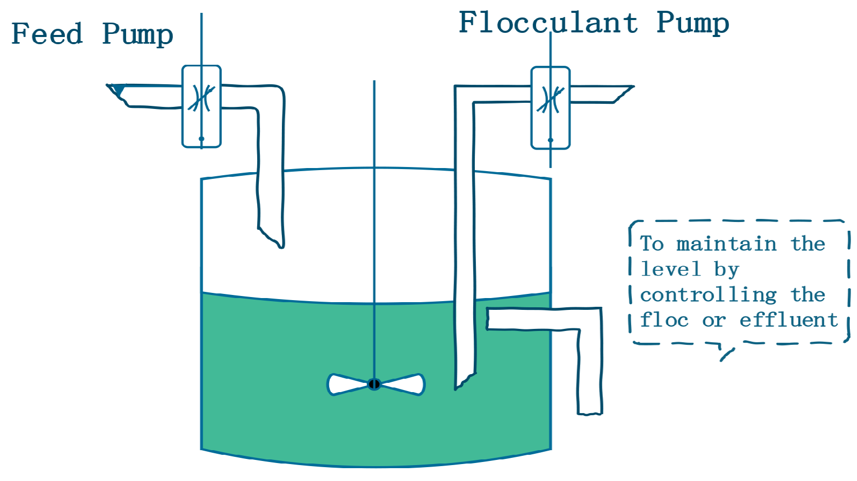
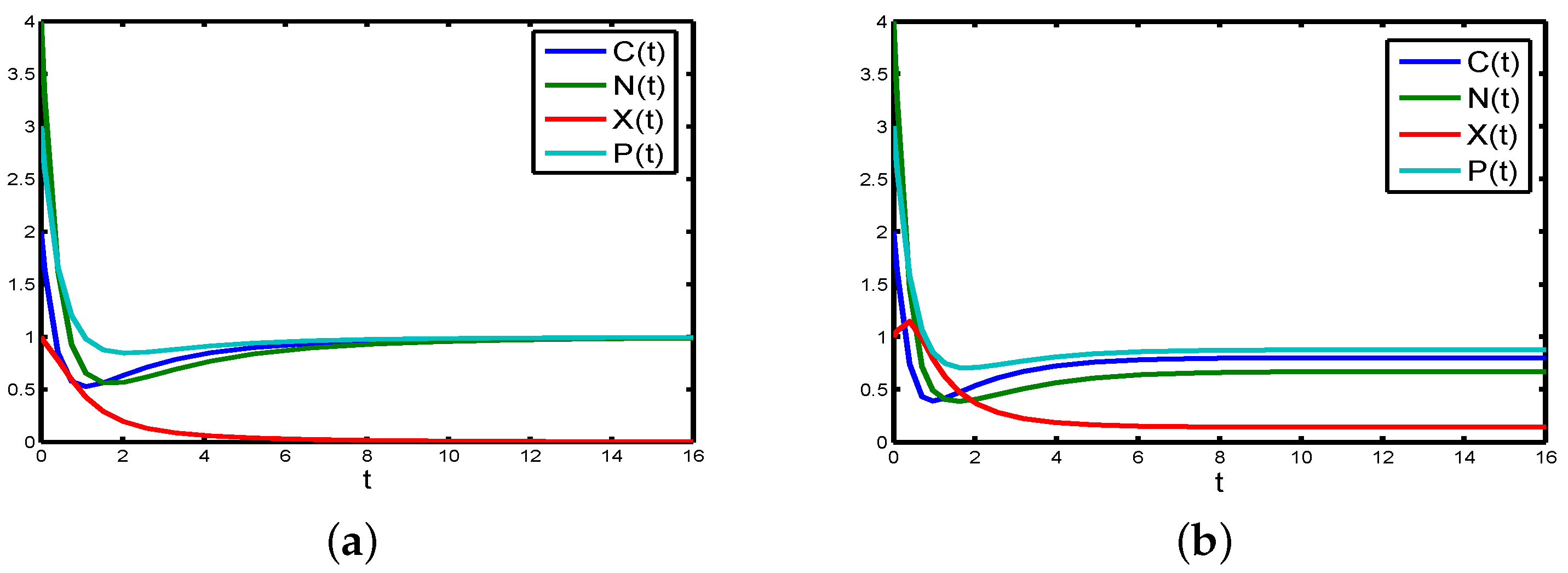
Remark 1. 
The existence of multiple positive equilibria of Model (4) when R 0 < 1 (shown in Table A1; see Appendix A) indicates the possibility of the existence of backward bifurcation (see, for example, [40,47,48]), where the stable boundary equilibrium co-exists with a stable positive equilibrium. This can be explored below via numerical simulations (see Figure 2a,b). A rigorous result can be obtained using center manifold theory [49]. The detailed proof is given in Appendix B.
From the analysis given in Appendix B, we have established the following result.
Theorem 4. 
(i)
If:
m 1 m 2 > r r 1 K 1 ( K 1 + 1 ) 3 ( K 2 + 1 ) 2 + r r 2 K 2 ( K 1 + 1 ) 2 ( K 2 + 1 ) 3 ,
then Model (4) undergoes a backward bifurcation at R 0 = 1 .
(ii)
If:
m 1 m 2 < r r 1 K 1 ( K 1 + 1 ) 3 ( K 2 + 1 ) 2 + r r 2 K 2 ( K 1 + 1 ) 2 ( K 2 + 1 ) 3 ,
then Model (4) undergoes a forward bifurcation at R 0 = 1 .
The existence of backward bifurcation implies that stable boundary equilibrium and stable positive equilibrium may be coexistent. In biology, this means that the basic bifurcation parameter R 0 is not the threshold value, which is used to determine whether R h o d o p s e u d o m o n a s p a l u s t r i s can be harvested successfully or not. In this case, more complicated dynamic properties may occur. There may exist a new threshold value, which is less than R 0 and used to determine whether R h o d o p s e u d o m o n a s p a l u s t r i s can be harvested successfully or not.

4. The Global Stability of the Boundary Equilibrium

Global stability properties of the equilibria E 0 or E * imply that the asymptotic properties of the carbon source, nitrogen source, R h o d o p s e u d o m o n a s p a l u s t r i s and flocculants in the culture vessel are not dependent on the initial values C 0 , N 0 , X 0 and P 0 . For the global stability property of the boundary equilibrium E 0 of Model (4), we have the following result.
Theorem 5. 
If R 0 < 1 , then the boundary equilibrium E 0 ( 1 , 1 , 0 , 1 ) of Model (4) is locally asymptotically stable. Further, if:
R 0 m 1 P ̲ + 1 m 1 + 1 < 1 ,
then the boundary equilibrium E 0 of Model (4) is globally asymptotically stable.
Proof. 
It is easy to show that the boundary equilibrium E 0 ( 1 , 1 , 0 , 1 ) of Model (4) is locally asymptotically stable by the characteristic equation of the linearization of Model (4). Next, we prove the global asymptotic stability of the boundary equilibrium E 0 of Model (4).
Since Ω is attractive and positively forward invariant for Model (4), hence it just considers Model (4) in Ω. Define:
V 1 = X .
Apparently, V 1 ( 1 , 1 , 0 , 1 ) = 0 and V 1 is continuous on Ω. If R 0 m 1 P ̲ + 1 m 1 + 1 < 1 , then the derivative of V 1 along the solutions of Model (4) is:
V ˙ 1 = r C ( t ) N ( t ) X ( t ) ( K 1 + C ( t ) ) ( K 2 + N ( t ) ) - X ( t ) - m 1 X ( t ) P ( t ) ( r C ( t ) N ( t ) ( K 1 + C ( t ) ) ( K 2 + N ( t ) ) - 1 - m 1 P ̲ ) X ( t ) ( m 1 + 1 ) ( r C ( t ) N ( t ) ( K 1 + C ( t ) ) ( K 2 + N ( t ) ) 1 m 1 + 1 - R 0 ) X ( t ) ( m 1 + 1 ) ( r ( K 1 + 1 ) ( K 2 + 1 ) 1 m 1 + 1 - R 0 ) X ( t ) = 0
for any t 0 . Hence, V 1 is a Lyapunov function of Model (4) on Ω.
Define E = { ( C , N , X , P ) | ( C , N , X , P ) Ω , V ˙ 1 = 0 } . We have that:
E { ( C , N , X , P ) | ( C , N , X , P ) Ω , X = 0 , or C = 1 and N = 1 } .
Let M ^ be the largest set in E, which is invariant with respect to Model (4). Clearly, M ^ is not empty, since ( 1 , 1 , 0 , 1 ) M ^ . For any ( C 0 , N 0 , X 0 , P 0 ) M ^ , let ( C ( t ) , N ( t ) , X ( t ) , P ( t ) ) be the solution of Model (4) with the initial Condition (5). From the invariance of M ^ , we get ( C ( t ) , N ( t ) , X ( t ) , P ( t ) ) M ^ E for any t R . Thus, we get, for each t, X ( t ) = 0 , or C ( t ) = 1 , and N ( t ) = 1 .
If for some t ˜ , C ( t ˜ ) = 1 and N ( t ˜ ) = 1 , then we have that C ˙ ( t ˜ ) = N ˙ ( t ˜ ) = 0 . Hence, from the first or second equation of Model (4), we obtain that X ( t ˜ ) = 0 . Thus, for any t R , we have that X ( t ) 0 .
Subsequently, from the first, second and forth equations of Model (4), we have that, for any t R ,
C ˙ ( t ) = 1 - C ( t ) , N ˙ ( t ) = 1 - N ( t ) , P ˙ ( t ) = 1 - P ( t ) .
Furthermore, for any t R , we have that:
C ( t ) = 1 - ( 1 - C ( 0 ) ) e - t , N ( t ) = 1 - ( 1 - N ( 0 ) ) e - t , P ( t ) = 1 - ( 1 - P ( 0 ) ) e - t .
If C ( 0 ) < 1 or N ( 0 ) < 1 or P ( 0 ) < 1 , then C ( t ) , N ( t ) and P ( t ) become negative values ( t - ) . Then, we obtain that C ( 0 ) = 1 , N ( 0 ) = 1 and P ( 0 ) = 1 . Hence, we obtain that, for any t R , C ( t ) = N ( t ) = P ( t ) 1 . Therefore, we obtain M ^ = { ( 1 , 1 , 0 , 1 ) } . The classical Lyapunov–LaSalle invariance principle shows that E 0 is globally attractive. Since it has been shown that, if R 0 m 1 P ̲ + 1 m 1 + 1 < 1 , the boundary equilibrium E 0 of Model (4) is locally asymptotically stable. Hence, the boundary equilibrium E 0 of Model (4) is globally asymptotically stable. □
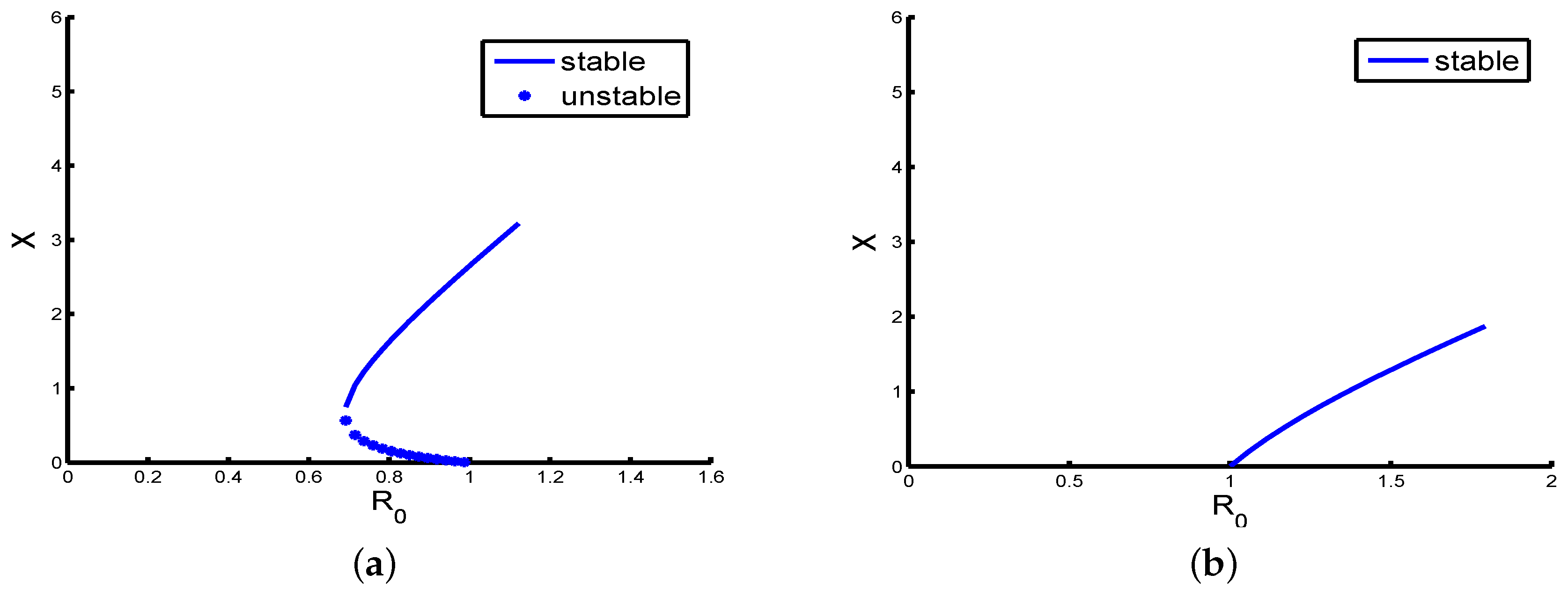
Remark 2. 
Let us use some numerical simulations to check the correctness of the theoretical analyses. We set
r = 1.5 , K 1 = 0.36 , K 2 = 0.3 , m 1 = 1.5 , m 2 = 4 , r 1 = 0.96 , r 2 = 1.0001 .
By the analysis of Theorem 5, we obtain that the boundary equilibrium E 0 of Model (4) is globally asymptotically stable (see Figure 3a).
Furthermore, if the parameters are chosen as follows, r = 3.5 , K 1 = 0.36 , K 2 = 0.3 , m 1 = 1.5 , m 2 = 4 , r 1 = 0.96 , r 2 = 1.0001 , it is easy to check that the condition R 0 < 1 holds, but there are two positive equilibria, E 1 * ( C * , N * , X * , P * ) ( 0.4783 , 0.4565 , 1.5782 , 0.1376 ) and E 2 * ( C * , N * , X * , P * ) ( 0.9100 , 0.9063 , 0.1741 , 0.5895 ) . Then, the backward bifurcation phenomenon is illustrated. Therefore, sufficient Condition (10) is reasonable.

5. Stability and Uniform Persistence

In this section, we give the local asymptotic stability of the positive equilibrium and uniform persistence of Model (4). Further, under additional conditions, the global asymptotic stability of the positive equilibrium is obtained by using some techniques of constructing Lyapunov functions.

5.1. The Local Asymptotic Stability of the Positive Equilibrium

For the local asymptotic stability of the positive equilibrium of Model (4), we have the following result.
Theorem 6. 
If the positive equilibrium E * ( C * , N * , X * , P * ) of Model (4) exists and the condition:
m 1 < K 1 ( 1 - C * ) P * C * ( K 1 + C * ) + K 2 ( 1 - N * ) P * N * ( K 2 + N * )
holds, then the positive equilibrium E * ( C * , N * , X * , P * ) of Model (4) is locally asymptotically stable.
Proof. 
For convenience, we assume that:
Δ = K 1 r 1 N * X * ( K 1 + C * ) 2 ( K 2 + N * ) + K 2 r 2 C * X * ( K 1 + C * ) ( K 2 + N * ) 2 .
For the linearized system, the corresponding characteristic equation of Model (4) can be expressed as follows:
λ 4 + A 1 λ 3 + A 2 λ 2 + A 3 λ + A 4 = 0 ,
where:
A 1 = 3 + m 2 X * + Δ , A 2 = Δ ( m 1 P * + 2 + m 2 X * ) + 1 + Δ + 2 ( 1 + m 2 X * ) - m 1 m 2 P * X * , A 3 = Δ ( 2 m 1 P * + 3 + 2 m 2 X * ) - 2 m 1 m 2 P * X * + 1 + m 2 X * , A 4 = m 2 X * ( Δ - m 1 P * ) + ( 1 + m 1 P * ) Δ .
According to the Routh-Hurwitz criterion, we need to show that:
A 1 A 2 - A 3 > 0 , A 3 ( A 1 A 2 - A 3 ) - A 1 2 A 4 > 0 , A 4 > 0 .
For the sake of simplicity, we define:
Δ 1 = A 1 , Δ 2 = A 1 A 2 - A 3 , Δ 3 = A 3 ( A 1 A 2 - A 3 ) - A 1 2 A 4 , Δ 4 = A 4 Δ 3 .
By computation, it can be obtained that:
Δ 1 = A 1 > 0 , Δ 2 = m 2 X * ( 1 + Δ + m 2 X * ) ( Δ - m 1 P * ) + ( 2 + 2 m 2 X * + Δ ) ( 3 + m 2 X * ) + Δ ( 6 + m 1 P * ) + Δ ( m 2 X * + Δ ) ( 3 + m 1 P * ) , Δ 3 = P 1 ( Δ - m 1 P * ) + Q , P 1 = 2 m 2 X * Δ ( 1 + Δ ) ( 3 + m 1 P * + m 2 X * ) + 4 m 2 X * 1 + Δ ( 1 + m 2 X * ) + 4 m 2 X * ( 1 + m 2 X * ) ( m 2 X * + 3 ) + 2 ( m 2 X * ) 2 Δ ( 1 + m 2 X * ) + m 2 X * Δ ( 1 + m 2 X * ) ( 2 m 1 P * + 3 + 2 m 2 X * ) , Q = a 1 ( 1 + m 1 P * ) + a 2 ( 3 + m 1 P * + m 2 X * ) + a 3 ( 1 + m 2 X * ) + a 4 m 1 P * m 2 X * Δ + 2 a 5 m 1 P * m 2 X * + a 6 m 2 X * Δ + Δ 2 ( 2 + 3 m 2 X * ) ( 3 + 2 m 2 X * ) + 14 Δ + 4 Δ 2 , a 1 = 2 Δ 3 + 8 Δ 2 + 7 Δ + m 2 X * Δ ( m 2 X * + 7 ) + m 1 P * Δ 2 ( Δ + 2 ) , a 2 = Δ ( 1 + Δ ) ( 1 + m 2 X * ) + Δ 3 ( 2 + m 1 P * ) + Δ 2 , a 3 = 2 1 + ( 1 + m 2 X * ) ( 3 + m 2 X * ) , a 4 = 2 ( m 2 X * ) 2 + ( 1 + Δ ) 2 , a 5 = 4 + ( m 2 X * ) 2 + m 1 P * m 2 X * + 2 m 2 X * , a 6 = 4 m 2 X * + 4 Δ + 13 , Δ 4 = A 4 Δ 3 .
If:
Δ = K 1 r 1 N * X * ( K 1 + C * ) 2 ( K 2 + N * ) + K 2 r 2 C * X * ( K 1 + C * ) ( K 2 + N * ) 2 > m 1 P * ,
that is,
m 1 < K 1 ( 1 - C * ) P * C * ( K 1 + C * ) + K 2 ( 1 - N * ) P * N * ( K 2 + N * ) ,
we obtain that Δ 1 > 0 , Δ 2 > 0 , Δ 3 > 0 , and Δ 4 > 0 . Hence, from the Routh-Hurwitz criterion, we obtain that the positive equilibrium E * ( C * , N * , X * , P * ) of Model (4) is locally asymptotically stable. This completes the proof of Theorem 6. □

5.2. Uniform Persistence

As pointed out in [29,45,50], uniform persistence is an important concept in the cultivation of microorganisms. From a biological perspective, one basic question about biological models involves the long-time survival of the species. To this end, we may want to know whether the constructed model is uniformly persistent with respect to one or more species. That is, the number of the species will keep positive and bounded away from zero for any positive time. In recent years, this kind of research has been particularly common in microorganisms (see, for example, [45]), especially in the simulation of harmful algae growth, where we usually want to predict if the harmful algae will go towards extinction or if blooms of the harmful algae will remain, which directly impacts human health and food webs in aquatic ecosystems. From a mathematical point of view, uniform persistence can give sufficient criteria for the existence of a positive equilibrium for the dissipative system [51].
Model (4) is said to be uniformly persistent if there are positive constants n 1 , n 2 , n 3 , n 4 , N 1 , N 2 , N 3 , N 4 , such that each positive solution ( C ( t ) , N ( t ) , X ( t ) , P ( t ) ) of Model (4) satisfies:
n 1 lim inf t C ( t ) lim sup t C ( t ) N 1 , n 2 lim inf t N ( t ) lim sup t N ( t ) N 2 , n 3 lim inf t X ( t ) lim sup t X ( t ) N 3 , n 4 lim inf t P ( t ) lim sup t P ( t ) N 4 .
Now, we give a result on the uniform persistence of Model (4). To proceed, we introduce the following notation and terminology. Denote by R ( t ) ( t 0 ) the family of solution operators corresponding to Model (4). The ω-limit set ω ( x ) of x consists of y , such that there exists a sequence t n as n with R ( t n ) x y as n . Define:
G = { ( C , N , X , P ) R + 4 C ̲ C 1 , N ̲ N 1 , X 0 , P ̲ P 1 } ,
G 0 = { ( C , N , X , P ) G C ̲ C 1 , N ̲ N 1 , X > 0 , P ̲ P 1 } ,
G 0 = G \ G 0 ,
M = { ( C , N , X , P ) G 0 R ( t ) ( C , N , X , P ) satisfies Model (4) and R ( t ) ( C , N , X , P ) G 0 , t 0 } ,
Ω ( M ) = x M ω ( x ) .
From Theorem 2, we obtain that G is positively invariant corresponding to R ( t ) . It is easy to see that G 0 is also positively invariant.
Clearly, G 0 is relatively compact in G. Now, we show that Ω ( M ) = { ( 1 , 1 , 0 , 1 ) } .
In fact, { ( 1 , 1 , 0 , 1 ) } Ω ( M ) . For any ( C ( 0 ) , N ( 0 ) , X ( 0 ) , P ( 0 ) ) M , it has that, for all t 0 , X ( t ) 0 and lim t + C ( t ) = lim t + N ( t ) = lim t + P ( t ) = 1 . Thus, Ω ( M ) = { ( 1 , 1 , 0 , 1 ) } .
Theorem 7. 
If R 0 > 1 , then Model (4) is uniformly persistent.
Proof. 
By Theorem 1, it can be obtained that nonnegative solutions of Model (4) are point dissipative. According to the definitions above, it suffices to show that G 0 repels uniformly nonnegative solutions of Model (4). It is obvious that there is only one equilibrium E 0 in M .
We now show that W s ( E 0 ) G 0 = . Assume W s ( E 0 ) G 0 , then there exists a positive solution of Model (4), such that lim t ( C ( t ) , N ( t ) , X ( t ) , P ( t ) ) = ( 1 , 1 , 0 , 1 ) . Assume:
U ( C ( t ) , N ( t ) , P ( t ) ) = r C ( t ) N ( t ) ( K 1 + C ( t ) ) ( K 2 + N ( t ) ) - 1 - m 1 P ( t ) ,
then:
U ( 1 , 1 , 1 ) = r ( K 1 + 1 ) ( K 2 + 1 ) - 1 - m 1 .
Then, r > ( K 1 + 1 ) ( K 2 + 1 ) ( 1 + m 1 ) is equivalent to U ( 1 , 1 , 1 ) > 0 .
Since lim t U ( C ( t ) , N ( t ) , P ( t ) ) = U ( 1 , 1 , 1 ) > 0 , there exists T > 0 , such that, for any t T ,
U ( C ( t ) , N ( t ) , P ( t ) ) > 1 2 U ( 1 , 1 , 1 ) > 0 .
By the third equation of Model (4), we obtain that, for any t T ,
X ˙ ( t ) = r C ( t ) N ( t ) X ( t ) ( K 1 + C ( t ) ) ( K 2 + N ( t ) ) - X ( t ) - m 1 P ( t ) X ( t ) = U ( C ( t ) , N ( t ) , P ( t ) ) X ( t ) > 1 2 U ( 1 , 1 , 1 ) X ( t ) .
This implies that X ( t ) + as t + , which leads to a contradiction. Thus, W s ( E 0 ) G 0 = .
In the following, let us show that E 0 is factually isolated. That is, there exists some neighborhood U of E 0 , such that E 0 is the largest invariant set in U. In fact, for sufficiently small positive constant ε, let us choose:
U = U ( E 0 ) = { ( C , N , X , P ) G | 1 - C < ε , 1 - N < ε , X < ε , 1 - P < ε } .
We show that E 0 is the largest invariant set of U for some ε .
If not, for any sufficiently small ε, there exists some invariant set W ( W U ) , such that W \ E 0 is not empty. Let ( C 0 , N 0 , X 0 , P 0 ) W \ E 0 and ( C ( t ) , N ( t ) , X ( t ) , P ( t ) ) be the solution of Model (4) with the initial function (5). Then, we have that ( C ( t ) , N ( t ) , X ( t ) , P ( t ) ) U , t ( - , + ) . From the third equation of Model (4), we obtain that, for t ( - , + ) ,
X ˙ ( t ) r ( 1 - ε ) ( 1 - ε ) X ( t ) ( K 1 + 1 - ε ) ( K 2 + 1 - ε ) - X ( t ) - m 1 X ( t ) .
Since r > ( K 1 + 1 ) ( K 2 + 1 ) ( m 1 + 1 ) , we can choose sufficiently small ε, such that:
r ( 1 - ε ) ( 1 - ε ) > ( K 1 + 1 - ε ) ( K 2 + 1 - ε ) ( 1 + m 1 ) .
If X 0 > 0 , then we have X ( t ) + ( t + ) , which contracts the boundedness of X ( t ) . Hence, we get X 0 = 0 . From the third equation of Model (4), we obtain that X ( t ) 0 . From the first, second and forth equations of Model (4), for t ( - , + ) , we obtain that C ˙ ( t ) = 1 - C ( t ) , N ˙ ( t ) = 1 - N ( t ) and P ˙ ( t ) = 1 - P ( t ) . Hence, we must have that C 0 = N 0 = P 0 = 1 . Therefore, ( C 0 , N 0 , X 0 , P 0 ) = ( 1 , 1 , 0 , 1 ) , which is a contradiction. Thus, we obtain that E 0 is factually isolated.
Clearly, E 0 is acyclic in M . By paper [52], G 0 repels uniformly nonnegative solutions of Model (4). It then follows that Model (4) is persistent.
Define p : X R + by p ( C , N , X , P ) = X , ( C , N , X , P ) G . Obviously, we obtain that G 0 = p - 1 ( 0 , + ) and G 0 = p - 1 ( 0 ) . Thus, by ([53], Theorem 3), we have lim inf t ( C ( t ) , N ( t ) , X ( t ) , P ( t ) ) ( η , η , η , η ) . It then follows that Model (4) is uniformly persistent. The proof of Theorem 7 is completed. □
According to [51,53], we easily obtain the following result.
Corollary 8. 
If R 0 > 1 , then Model (4) has one global attractor A 0 and also has at least one positive equilibrium E * ( C * , N * , X * , P * ) A 0 .

5.3. The Global Asymptotic Stability of the Positive Equilibrium

In this subsection, the global asymptotic stability of the positive equilibrium E * ( C * , N * , X * , P * ) of Model (4) is studied.
Theorem 9. 
Assume that R 0 > 1 and Model (4) has a unique positive equilibrium E * ( C * , N * , X * , P * ) . Let:
D 1 = r 1 ( 2 + m 1 P * ) ( K 1 + C * ) ( K 2 + N * ) - r 2 N * , D 2 = r 2 ( 2 + m 1 P * ) ( K 1 + C * ) ( K 2 + N * ) - r 2 , D 3 = b 13 2 + b 23 2 + 4 b 33 , D 4 = 4 b 33 b 44 + ( b 23 2 + b 13 2 ) b 44 + ( b 14 2 + b 24 2 ) b 33 - b 34 2 + b 23 b 24 b 34 + b 13 b 14 b 34 .
If D 1 0 , D 2 0 , D 3 < 0 and D 4 > 0 hold, then the positive equilibrium E * ( C * , N * , X * , P * ) of Model (4) is globally asymptotically stable. Here:
b 13 = 2 r 1 + r 1 m 1 P * r + r ( K 1 + 1 ) ( K 2 + 1 ) ( K 1 + C * ) - r N * ( K 1 + C * ) ( K 2 + N * ) , b 14 = r 1 m 1 α r , b 23 = 2 r 2 + r 2 m 1 P * r , b 24 = r 2 m 1 α r , b 33 = - ( r 1 2 + r 2 2 ) ( 1 + m 1 P * ) r 2 , b 34 = ( r 1 2 + r 2 2 ) m 1 α r 2 + m 1 + m 2 , b 44 = - ( 1 + m 2 X * ) .
Proof. 
Let us consider the following Lyapunov function on A 0 ,
V 2 = 1 2 C - C * + r 1 r ( X - X * ) 2 + 1 2 N - N * + r 2 r ( X - X * ) 2 + X - X * - X * ln X X * + P - P * - P * ln P P * .
Clearly, V 2 ( C * , N * , X * , P * ) = 0 , and V 2 is positive definite with respect to E * ( C * , N * , X * , P * ) . The derivative of V 2 along the solutions of Model (4) is:
V ˙ 2 = C ( t ) - C * + r 1 r ( X ( t ) - X * ) C ˙ ( t ) + r 1 r X ˙ ( t ) + N ( t ) - N * + r 2 r ( X ( t ) - X * ) N ˙ ( t ) + r 2 r X ˙ ( t ) + X ( t ) - X * X ( t ) X ˙ ( t ) + P ( t ) - P * P ( t ) P ˙ ( t ) = C ( t ) - C * + r 1 r ( X ( t ) - X * ) 1 - C ( t ) - r 1 r X ( t ) - r 1 m 1 X ( t ) P ( t ) r + N ( t ) - N * + r 2 r ( X ( t ) - X * ) 1 - N ( t ) - r 2 r X ( t ) - r 2 m 1 X ( t ) P ( t ) r + ( X ( t ) - X * ) r C ( t ) N ( t ) ( K 1 + C ( t ) ) ( K 2 + N ( t ) ) - 1 - m 1 P ( t ) + P ( t ) - P * P ( t ) ( 1 - P ( t ) - m 2 X ( t ) P ( t ) )
for any t 0 .
Noting that:
1 - C * - r 1 C * N * X * ( K 1 + C * ) ( K 2 + N * ) = 0 , 1 - N * - r 2 C * N * X * ( K 1 + C * ) ( K 2 + N * ) = 0 , r C * N * X * ( K 1 + C * ) ( K 2 + N * ) - X * - m 1 X * P * = 0 , 1 - P * - m 2 X * P * = 0 .
Thus, we have that:
V ˙ 2 = C ( t ) - C * + r 1 r ( X ( t ) - X * ) C * - C ( t ) + r 1 r ( X * - X ( t ) ) + r 1 m 1 r ( X * P * - X ( t ) P ( t ) ) + N ( t ) - N * + r 2 r ( X ( t ) - X * ) N * - N ( t ) + r 2 r ( X * - X ( t ) ) + r 2 m 1 r ( X * P * - X ( t ) P ( t ) ) + ( X ( t ) - X * ) r C ( t ) N ( t ) ( K 1 + C ( t ) ) ( K 2 + N ( t ) ) - r C * N * ( K 1 + C * ) ( K 2 + N * ) + m 1 ( X ( t ) - X * ) ( P * - P ( t ) ) + P ( t ) - P * P ( t ) P * - P ( t ) + m 2 ( X * P * - X ( t ) P ( t ) )
for any t 0 .
For any t 0 , we have that:
r C ( t ) N ( t ) ( K 1 + C ( t ) ) ( K 2 + N ( t ) ) - r C * N * ( K 1 + C * ) ( K 2 + N * ) = - r C * N * ( K 1 + C * ) ( K 2 + N * ) + r C ( t ) N * ( K 1 + C * ) ( K 2 + N * ) - r C ( t ) N * ( K 1 + C * ) ( K 2 + N * ) + r C ( t ) N ( t ) ( K 1 + C * ) ( K 2 + N * ) - r C ( t ) N ( t ) ( K 1 + C * ) ( K 2 + N * ) + r C ( t ) N ( t ) ( K 1 + C * ) ( K 2 + N ( t ) ) - r C ( t ) N ( t ) ( K 1 + C * ) ( K 2 + N ( t ) ) + r C ( t ) N ( t ) ( K 1 + C ( t ) ) ( K 2 + N ( t ) ) .
Hence, it can be obtained that, for any t 0 ,
V ˙ 2 = C ( t ) - C * + r 1 r ( X ( t ) - X * ) ( C * - C ( t ) + r 1 r ( X * - X ( t ) ) + r 1 m 1 P * r ( X * - X ( t ) ) + r 1 m 1 X ( t ) r ( P * - P ( t ) ) ) + N ( t ) - N * + r 2 r ( X ( t ) - X * ) ( N * - N ( t ) + r 2 r ( X * - X ( t ) ) + r 2 m 1 P * r ( X * - X ( t ) ) + r 2 m 1 X ( t ) r ( P * - P ( t ) ) ) + ( X ( t ) - X * ) ( - r C * N * ( K 1 + C * ) ( K 2 + N * ) + r C ( t ) N * ( K 1 + C * ) ( K 2 + N * ) - r C ( t ) N * ( K 1 + C * ) ( K 2 + N * ) + r C ( t ) N ( t ) ( K 1 + C * ) ( K 2 + N * ) - r C ( t ) N ( t ) ( K 1 + C * ) ( K 2 + N * ) + r C ( t ) N ( t ) ( K 1 + C * ) ( K 2 + N ( t ) ) - r C ( t ) N ( t ) ( K 1 + C * ) ( K 2 + N ( t ) ) + r C ( t ) N ( t ) ( K 1 + C ( t ) ) ( K 2 + N ( t ) ) ) - ( P ( t ) - P * ) 2 P ( t ) + m 2 ( P ( t ) - P * ) P ( t ) X * ( P * - P ( t ) ) + P ( t ) ( X * - X ( t ) ) + m 1 ( X ( t ) - X * ) ( P * - P ( t ) ) .
Motivated by the papers mentioned in [50,54], the derivative of V 2 along the solutions of Model (4) is represented in quadratic form. Then, we obtain that:
V ˙ 2 = - ( C ( t ) - C * ) 2 - ( N ( t ) - N * ) 2 + ( 2 r 1 + r 1 m 1 P * r + r C ( t ) N ( t ) ( K 1 + C ( t ) ) ( K 2 + N ( t ) ) ( K 1 + C * ) - r N * ( K 1 + C * ) ( K 2 + N * ) ) ( C ( t ) - C * ) ( X * - X ( t ) ) + ( 2 r 2 + r 2 m 1 P * r + r C ( t ) N ( t ) ( K 2 + N ( t ) ) ( K 2 + N * ) ( K 1 + C * ) - r C ( t ) ( K 1 + C * ) ( K 2 + N * ) ) ( N ( t ) - N * ) ( X * - X ( t ) ) - 1 + m 2 X * P ( t ) ( P ( t ) - P * ) 2 + r 1 m 1 X r ( C ( t ) - C * ) ( P * - P ( t ) ) - ( r 1 2 + r 2 2 ) ( 1 + m 1 P * ) r 2 ( X ( t ) - X * ) 2 + ( r 1 2 + r 2 2 ) m 1 X ( t ) r 2 + m 1 + m 2 ( X * - X ( t ) ) ( P * - P ( t ) ) + r 2 m 1 X ( t ) r ( N ( t ) - N * ) ( P * - P ( t ) )
for any t 0 .
If the condition D 1 0 holds, we obtain that, for any t 0 ,
2 r 1 + r 1 m 1 P * r + r C ( t ) N ( t ) ( K 1 + C ( t ) ) ( K 2 + N ( t ) ) ( K 1 + C * ) - r N * ( K 1 + C * ) ( K 2 + N * ) 0 .
Furthermore, from the condition D 2 0 and C ( t ) 1 for any t 0 , we obtain that:
2 r 2 + r 2 m 1 P * r + r C ( t ) N ( t ) ( K 2 + N ( t ) ) ( K 2 + N * ) ( K 1 + C * ) - r C ( t ) ( K 1 + C * ) ( K 2 + N * ) 0 .
These conditions ensure that the coefficients of ( C ( t ) - C * ) ( X ( t ) - X * ) and ( N ( t ) - N * ) ( X ( t ) - X * ) are nonnegative. Thus, we obtain that, for any t 0 ,
V ˙ 2 - ( C ( t ) - C * ) 2 - ( N ( t ) - N * ) 2 + ( 2 r 1 + r 1 m 1 P * r + r ( K 1 + 1 ) ( K 2 + 1 ) ( K 1 + C * ) - r N * ( K 1 + C * ) ( K 2 + N * ) ) C ( t ) - C * X * - X ( t ) + ( 2 r 2 + r 2 m 1 P * r ) N ( t ) - N * X * - X ( t ) - ( 1 + m 2 X * ) ( P ( t ) - P * ) 2 + r 1 m 1 α r C ( t ) - C * P * - P ( t ) - ( r 1 2 + r 2 2 ) ( 1 + m 1 P * ) r 2 ( X ( t ) - X * ) 2 + ( r 1 2 + r 2 2 ) m 1 α r 2 + m 1 + m 2 X * - X ( t ) P * - P ( t ) + r 2 m 1 α r N ( t ) - N * P * - P ( t ) = Y T ( t ) W Y ( t ) ,
where Y ( t ) = ( C ( t ) - C * , N ( t ) - N * , X ( t ) - X * , P ( t ) - P * ) . W is a symmetric 4 × 4 matrix and W = { b i j } 1 i , j 4 with:
W = b 11 1 2 b 12 1 2 b 13 1 2 b 14 1 2 b 12 b 22 1 2 b 23 1 2 b 24 1 2 b 13 1 2 b 23 b 33 1 2 b 34 1 2 b 14 1 2 b 24 1 2 b 34 b 44 .
Here, b 11 = - 1 , b 12 = 0 , b 22 = - 1 . The other parameters have the same definitions as in Theorem 9. Then, W is negative definite. By Lemma 6.2 provided in [50], we can obtain that the real quadratic form Y T ( t ) W Y ( t ) is negative definite. Then, by using some classical analysis techniques of differential equations, the positive equilibrium E * ( C * , N * , X * , P * ) of Model (4) is globally asymptotically stable. □
Remark 3. 
Obviously, it is easy to obtain that b 11 = - 1 < 0 , and:
b 11 1 2 b 12 1 2 b 12 b 22 = 1 > 0 .
If the conditions D 3 < 0 and D 4 > 0 hold, we obtain that:
b 11 1 2 b 12 1 2 b 13 1 2 b 12 b 22 1 2 b 23 1 2 b 13 1 2 b 23 b 33 < 0 ,
and:
b 11 1 2 b 12 1 2 b 13 1 2 b 14 1 2 b 12 b 22 1 2 b 23 1 2 b 24 1 2 b 13 1 2 b 23 b 33 1 2 b 34 1 2 b 14 1 2 b 24 1 2 b 34 b 44 > 0 .
Next, we illustrate that the conditions given in Theorem 9 are reasonable. We set r = 5.8 , K 1 = 1 , K 2 = 0.6 , m 1 = 0.0001 , m 2 = 1 , r 1 = 6 , r 2 = 10 . It is easy to see that there exists a unique positive equilibrium E * ( C * , N * , X * , P * ) ( 0.6709 , 0.4515 , 0.3181 , 0.7587 ) , and the conditions D 1 D 4 hold. By Theorem 9, the positive equilibrium of Model (4) is globally asymptotically stable (see Figure 3b).
In general, it is very difficult to obtain the global stability properties of the positive equilibrium of Model (4). In this paper, we have obtained the sufficient conditions to ensure the global stability properties of the positive equilibrium by constructing a suitable Lyapunov function. Because of the complexity of the conditions, it is difficult to grasp biological intuition. However, from the numerical simulations, we have found some interesting biological phenomena. The conditions D 1 D 4 can be satisfied if the flocculation rate of microorganisms ( m 1 ) is small enough (see, Figure 3b). From a biological point of view, these conditions are reasonable. For more detailed biological considerations, we will leave it for further investigation.

6. Control Strategies

In this section, some control strategies are provided by suitable theoretical analysis. If R 0 < 1 holds, then, we have from Theorem 5 that the boundary equilibrium E 0 of Model (4) is locally asymptotically stable. We note that the condition R 0 < 1 is equivalent to the following inequality,
R 0 = r ( K 1 + 1 ) ( K 2 + 1 ) ( m 1 + 1 ) < 1 .
All of the parameters r, K 1 , K 2 and m 1 in (12) are defined as in Model (4). (12) can be further written as the following form,
r ( K 1 C 0 + 1 ) ( K 2 N 0 + 1 ) ( m 1 P 0 + D ) < 1 .
Here, all of the parameters r, K 1 , K 2 , m 1 , C 0 , N 0 , P 0 and D in (13) are defined as in Model (3).
In view of the biological meanings of the parameters in Model (3) and Condition ( 13 ) , Theorem 5 indicates that the concentration of R h o d o p s e u d o m o n a s p a l u s t r i s in the chemostat tends to zero, and the concentration of the carbon source, nitrogen source and flocculants may tend to the constant values C 0 , N 0 and P 0 , respectively, as time t increases, if one of the following two cases occurs: (a) reducing the absorption of R h o d o p s e u d o m o n a s p a l u s t r i s or the carbon input concentration, or the nitrogen input concentration; (b) improving the velocity or the flocculation effect or flocculant input concentration. These cases are reasonable, since they imply the insufficient sources for R h o d o p s e u d o m o n a s p a l u s t r i s to grow. Hence, in the environmental science field, it can be used to remove algae and heavy metals.
From Theorem 7, we have that Model (3) is uniformly persistent if R 0 > 1 . This means that the concentrations of the carbon source, nitrogen source, R h o d o p s e u d o m o n a s p a l u s t r i s and flocculants in the chemostat may be ultimately maintained at some positive constant values, as time t increases, if one of the following two cases occurs: (a) improving the absorption of R h o d o p s e u d o m o n a s p a l u s t r i s , or the carbon input concentration, or the nitrogen input concentration; (b) reducing the velocity or the flocculation effect or flocculant input concentration.
These control strategies can be performed by numerical simulations.
In the following, for convenience, we simulate the extinction or persistence of microorganism ( X ( t ) ) numerically by using (12) and Model (4).
If the parameters are chosen as in Table A2 (see Appendix A), R h o d o p s e u d o m o n a s p a l u s t r i s in the chemostat will tend to extinction (see Figure 4a).
If the absorption of R h o d o p s e u d o m o n a s p a l u s t r i s (r) is improved from r = 5.8 to r = 8 and the other parameters are the same as Table A2, R h o d o p s e u d o m o n a s p a l u s t r i s in the chemostat will tend to be constant (see Figure 4b).
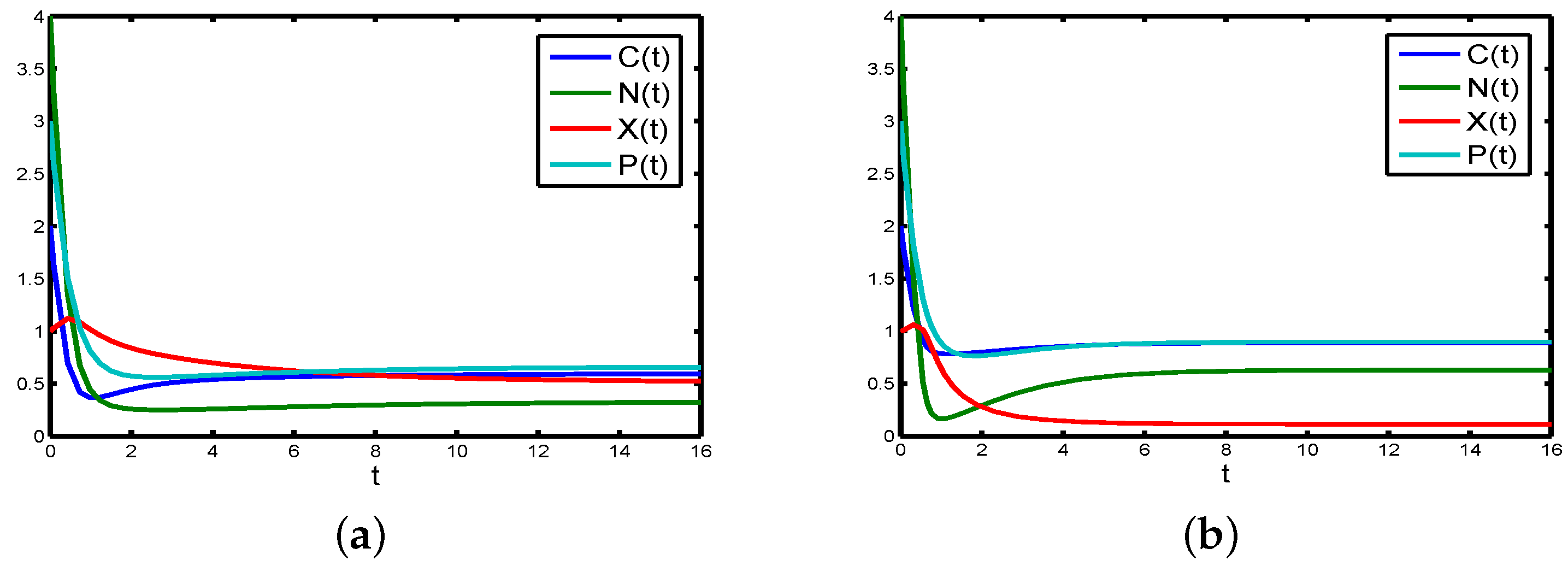
If the flocculation effect ( m 1 ) is reduced from m 1 = 1 to m 1 = 0.1 , R h o d o p s e u d o m o n a s p a l u s t r i s in the chemostat will tend to be constant (see Figure 5a).
If Michaelis–Menten constant of carbon ( K 1 ) is reduced from K 1 = 1 to K 1 = 0.5 , R h o d o p s e u d o m o n a s p a l u s t r i s in the chemostat will tend to be constant (see Figure 5b).
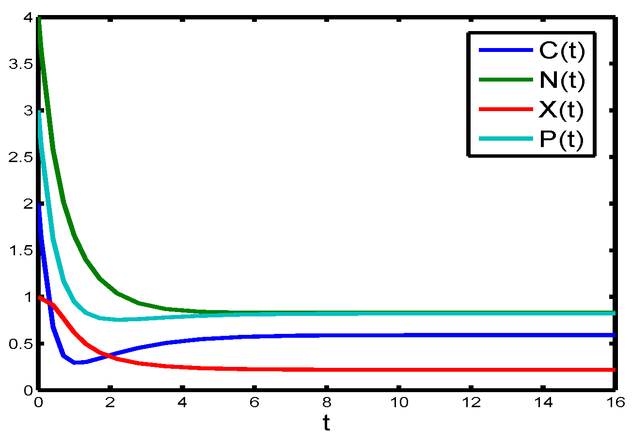
If Michaelis–Menten constant of nitrogen ( K 2 ) is reduced from K 2 = 1 to K 2 = 0.25 , R h o d o p s e u d o m o n a s p a l u s t r i s in the chemostat will tend to be constant (see Figure 6).

7. Discussion and Conclusions

In the paper, based on some biological considerations and chemostat models, a dynamic model governed by ordinary differential equations with four variables (carbon source, nitrogen source, R h o d o p s e u d o m o n a s p a l u s t r i s and flocculants) is presented. There is a boundary equilibrium and at most five positive equilibria for the proposed model. To give a theoretical analysis for the existence of all of the positive equilibria of Model (4), the method of the Descartes rule of signs is applied to the classifications of the positive roots of a fifth order algebraic equation.
The local and global stability properties of the boundary equilibrium of Model (4) have been studied in detail. An interesting phenomenon of backward and forward bifurcations is observed. That is, there may exist two positive equilibria even if the condition R 0 < 1 holds. Hence, sufficient Condition (10) to ensure the global stability of the boundary equilibrium is reasonable in mathematics.
The local stability of the positive equilibrium of Model (4) is also carried out. From Condition (11), we have that the positive equilibrium is locally asymptotically stable when the flocculation coefficient m 1 is small enough. Hence, Condition (11) is also reasonable in biology.
Uniform persistence of Model (4) has also been completely studied under the condition R 0 > 1 . Uniform persistence has very important significance both in mathematics and biology, and it characterizes the long-term survival of some microorganisms [45].
Finally, some control strategies are provided by simple theoretical analysis. From Theorem 5, we have that R h o d o p s e u d o m o n a s p a l u s t r i s in the chemostat will tend to extinction if R 0 < 1 . In this case, these control strategies can be applied to remove C y a n o b a c t e r i a , which are well known to produce a variety of toxins and have serious harm on human health. From Theorem 7, we have that R h o d o p s e u d o m o n a s p a l u s t r i s in the chemostat will tend to be positive constant if R 0 > 1 . In this case, these control strategies can be widely used for the collection of useful microorganisms.
It is well-known that the existence of time delays is inevitable in biology. For example, in the cultivation of microorganisms, there are always time delays in the process of transferring nutrients and the uptake of nutrients. Hence, chemostat models with time delays that account for the time lapsing between the uptake of nutrients by cells and the incorporation of these nutrients as biomass have been given much attention [40,55,56,57]. Based on Model (3), it may have the following more general form with time delays,
d C ( t ) d t = ( C 0 - C ( t ) ) D - r 1 C ( t ) N ( t ) X ( t ) δ 1 ( K 1 + C ( t ) ) ( K 2 + N ( t ) ) + ρ 1 X ( t - σ ) , d N ( t ) d t = ( N 0 - N ( t ) ) D - r 2 C ( t ) N ( t ) X ( t ) δ 2 ( K 1 + C ( t ) ) ( K 2 + N ( t ) ) + ρ 2 X ( t - σ ) , d X ( t ) d t = r e - d 1 τ C ( t - τ ) N ( t - τ ) X ( t - τ ) ( K 1 + C ( t - τ ) ) ( K 2 + N ( t - τ ) ) - D X ( t ) - d 1 X ( t ) - m 1 X ( t ) P ( t ) , d P ( t ) d t = ( P 0 - P ( t ) ) D - m 2 X ( t ) P ( t ) .
In Model (14), the constants ρ 1 0 and ρ 2 0 are the rate constants at which the carbon source and nitrogen source are recycled because of the death of R h o d o p s e u d o m o n a s p a l u s t r i s . The constant σ 0 is a fixed time during which the carbon source and nitrogen source are released completely from dead R h o d o p s e u d o m o n a s p a l u s t r i s . The constant τ 0 denotes the time delay involved in the conversion of nutrients to R h o d o p s e u d o m o n a s p a l u s t r i s . The factor e - d 1 τ is the probability constant at which R h o d o p s e u d o m o n a s p a l u s t r i s remains in the culture vessel during the conversion process. The theoretical analysis of Model (14) will be studied separately.

Acknowledgments

The authors thank the editors and anonymous reviewers for their valuable comments, especially for the biological considerations, numerical simulations and the proofs of the main results. The second author is supported by the National Natural Science Foundation of China (11471034).

Author Contributions

Wei Wang and Wanbiao Ma conceived of the study, drafted the manuscript and finished the mathematical analysis and numerical simulations. Hai Yan gave some suggestions for constructing the model.

Conflicts of Interest

The authors declare no conflict of interest.

Appendix A

In this section, let us apply the Descartes rule of signs to the classifications of the positive roots of f ( X * ) [47]. Let m represent the number of sign changes of the coefficients a , b , c , d , e , f of f ( X * ) and n represent the number of the positive roots.
Table A1. The number of the positive roots of f ( X * ) for R 0 < 1 and R 0 > 1 .
CasesabcdefR0mn
1+++++ R 0 < 1 11
++++ R 0 > 1 2 0 , 2
2++++ R 0 < 1 3 1 , 3
+++ R 0 > 1 2 0 , 2
3++++ R 0 < 1 3 1 , 3
+++ R 0 > 1 4 0 , 2 , 4
4+++ R 0 < 1 3 1 , 3
++ R 0 > 1 2 0 , 2
5++++ R 0 < 1 3 1 , 3
+++ R 0 > 1 4 0 , 2 , 4
6+++ R 0 < 1 5 1 , 3 , 5
++ R 0 > 1 4 0 , 2 , 4
7+++ R 0 < 1 3 1 , 3
++ R 0 > 1 4 0 , 2 , 4
8++ R 0 < 1 3 1 , 3
+ R 0 > 1 2 0 , 2
9++++ R 0 < 1 11
+++ R 0 > 1 2 0 , 2
10+++ R 0 < 1 3 1 , 3
++ R 0 > 1 2 0 , 2
11+++ R 0 < 1 3 1 , 3
++ R 0 > 1 4 0 , 2 , 4
12++ R 0 < 1 3 1 , 3
+ R 0 > 1 2 0 , 2
13+++ R 0 < 1 11
++ R 0 > 1 2 0 , 2
14++ R 0 < 1 3 1 , 3
+ R 0 > 1 2 0 , 2
15++ R 0 < 1 11
+ R 0 > 1 2 0 , 2
16+ R 0 < 1 11
R 0 > 1 00
Table A2. Parameter values used in the simulations of control strategies shown in Figure 3, Figure 4, Figure 5 and Figure 6.
DescriptionParameterValue
the growth rate of R h o d o p s e u d o m o n a s p a l u s t r i s r5.8
the quantity of decreasing of carbon source r 1 6
the quantity of decreasing of nitrogen source r 2 10
the flocculation effect m 1 1
the flocculation ratio m 2 1
Michaelis–Menten constant of carbon K 1 1
Michaelis–Menten constant of nitrogen K 2 0.6

Appendix B

In Section 3, we have discussed the phenomena of backward and forward bifurcations by numerical simulations. In this section, the center manifold theory is used on Model (4) to obtain the rigorous result (see, for example, [40,47,48]).
Let C = x 1 , N = x 2 , X = x 3 , P = x 4 , so that Model (4) can be re-written in the following form:
d x 1 ( t ) d t = 1 - x 1 - r 1 x 1 x 2 x 3 ( K 1 + x 1 ) ( K 2 + x 2 ) = g 1 , d x 2 ( t ) d t = 1 - x 2 - r 2 x 1 x 2 x 3 ( K 1 + x 1 ) ( K 2 + x 2 ) = g 2 , d x 3 ( t ) d t = r x 1 x 2 x 3 ( K 1 + x 1 ) ( K 2 + x 2 ) - x 3 - m 1 x 3 x 4 = g 3 , d x 4 ( t ) d t = 1 - x 4 - m 2 x 3 x 4 = g 4 .
The Jacobian matrix of Model (15) at E 0 ( 1 , 1 , 0 , 1 ) is given by:
J ( E 0 ) = - 1 0 - r 1 ( K 1 + 1 ) ( K 2 + 1 ) 0 0 - 1 - r 2 ( K 1 + 1 ) ( K 2 + 1 ) 0 0 0 r ( K 1 + 1 ) ( K 2 + 1 ) - 1 - m 1 0 0 0 - m 2 - 1 .
Suppose r is chosen as a bifurcation parameter. Solving R 0 = 1 gives:
r = r * = ( K 1 + 1 ) ( K 2 + 1 ) ( m 1 + 1 ) .
Eigenvectors of J ( E 0 ) | r = r *
It can be shown that the Jacobian matrix of Model (15) at r = r * has a right eigenvector (corresponding to the zero eigenvalue) given by ω = ( ω 1 , ω 2 , ω 3 , ω 4 ) T , where:
ω 1 = - r 1 ( K 1 + 1 ) ( K 2 + 1 ) ω 3 , ω 2 = - r 2 ( K 1 + 1 ) ( K 2 + 1 ) ω 3 , ω 3 = ω 3 > 0 , ω 4 = - m 2 ω 3 .
Further, the Jacobian matrix of Model (15) at r = r * has a left eigenvector (associated with the zero eigenvalue) given by v = ( v 1 , v 2 , v 3 , v 4 ) T , where:
v 1 = 0 , v 2 = 0 , v 3 = v 3 > 0 , v 4 = 0 .
Computations of a ^ and b ^
For Model (15), the associated non-zero partial derivatives of g = ( g 1 , g 2 , g 3 , g 4 ) T (at E 0 ) are given by:
2 g 3 x 1 x 3 = r K 1 ( K 1 + 1 ) 2 ( K 2 + 1 ) , 2 g 3 x 2 x 3 = r K 2 ( K 1 + 1 ) ( K 2 + 1 ) 2 , 2 g 3 x 3 x 4 = - m 1 , 2 g 3 x 3 r * = 1 ( K 1 + 1 ) ( K 2 + 1 ) .
It follows from the above expressions that:
a ^ = v 3 i = 1 , j = 1 4 ω i ω j 2 g 3 x i x j = 2 v 3 ω 1 ω 3 r K 1 ( K 1 + 1 ) 2 ( K 2 + 1 ) + ω 2 ω 3 r K 2 ( K 1 + 1 ) ( K 2 + 1 ) 2 - ω 3 ω 4 m 1 = 2 v 3 ω 3 2 m 1 m 2 - r r 1 K 1 ( K 1 + 1 ) 3 ( K 2 + 1 ) 2 - r r 2 K 2 ( K 1 + 1 ) 2 ( K 2 + 1 ) 3 ,
from which it can be shown that a ^ > 0 if:
m 1 m 2 > r r 1 K 1 ( K 1 + 1 ) 3 ( K 2 + 1 ) 2 + r r 2 K 2 ( K 1 + 1 ) 2 ( K 2 + 1 ) 3 .
For the sign of b ^ , it can be shown that the associated non-vanishing partial derivatives of g are:
b ^ = v 3 i = 1 4 ω i 2 g 3 x i r * = 2 v 3 ω 3 ( K 1 + 1 ) ( K 2 + 1 ) > 0 .
Thus, we have established Theorem 4 in view of [48]. The proof is completed.

References

  1. Wang, L.; Liao, L. Separation and identification of photosynthetic bacteria (PSB) and purifying effection aquiculture water. J. Microbiol. 2004, 2, 7–10. [Google Scholar]
  2. Takeno, K.; Sasaki, K.; Nishio, N. Removal of phosphorus from oyster farm mud sediment using a photosynthetic bacterium, Rhodobacter shaeroides IL106. J. Biosci. Bioeng. 1999, 88, 410–415. [Google Scholar] [CrossRef]
  3. Nagadomi, H.; Kitamura, T.; Watanabe, M.; Sasaki, K. Simultaneous removal of chemical oxygen demand (COD), phosphate, nitrate and hydrogen sulphide in the synthetic sewage wastewater using porous ceramic immobilized photosynthetic bacteria. Biotechnol. Lett. 2000, 22, 1369–1374. [Google Scholar] [CrossRef]
  4. Chen, F.; Jiang, Y. Microalgal Biotechnology; Chinese Light Industry Press: Beijing, China, 1999. [Google Scholar]
  5. Xu, F.; Zhang, S.; Zhang, P. Study of extracting CoQ10 from photosynthetic bacteria by ultrasonic assisted with zymolysis or freezing-thawing. Chem. Eng. 2008, 8, 43–45. [Google Scholar]
  6. Sasaki, K.; Watanabe, M.; Tanaka, T. Biosynthesis, biotechnological production and applications of 5-aminolevulinic acid. Appl. Microbiol. Biotechnol. 2012, 31, 119–123. [Google Scholar]
  7. Sasaki, K.; Watanabe, K.; Tanaka, T.; Tanaka, T. Effects of light sources on growth and carotenoid content of photosynthetic bacteria Rhodopseudomonas palustris. Bioresour. Technol. 2002, 58, 23–29. [Google Scholar]
  8. Carlozzi, P.; Sacchi, A. Biomass production and studies on Rhodopseudomonas palustris grown in an outdoor, temperature controlled, underwater tubular photobioreactor. J. Biotechnol. 2001, 3, 239–249. [Google Scholar] [CrossRef]
  9. Li, B.; Feng, J.; Xie, S. Degradation of microcystin by Rhodopseudomonas palustris. Chin. J. Ecol. 2012, 31, 119–123. [Google Scholar]
  10. Wu, S.C.; Liou, S.Z.; Lee, C.M. Correlation between bio-hydrogen production and polyhydroxybutyrate (PHB) synthesis by Rhodopseudomonas palustris WP3-5. Bioresour. Technol. 2012, 113, 44–50. [Google Scholar] [CrossRef] [PubMed]
  11. Kuo, F.S.; Chien, Y.H.; Chen, C. Effects of light sources on growth and carotenoid content of photosynthetic bacteria Rhodopseudomonas palustris. Bioresour. Technol. 2012, 113, 315–318. [Google Scholar] [CrossRef] [PubMed]
  12. Zhou, Q.; Zhang, P.; Zhang, G. Biomass and carotenoid production in photosynthetic bacteria wastewater treatment: Effects of light intensity. Bioresour. Technol. 2014, 171, 330–335. [Google Scholar] [CrossRef] [PubMed]
  13. Kong, F.; Song, L. Algal Blooms Process and Its Environmental Characteristics; Science Press: Beijing, China, 2011. [Google Scholar]
  14. Pan, G.; Zhang, M.; Chen, H.; Zou, H.; Yan, H. Removal of cyanobacterial blooms in Taihu Lake using local soils I. Equilibrium and kinetic screening on the flocculation of Microcystis aeruginosa using commercially available clays and minerals. Environ. Pollut. 2006, 141, 195–200. [Google Scholar] [CrossRef] [PubMed]
  15. Ghernaout, B.; Ghernaout, D.; Saiba, A. Algae and cyanotoxins removal by coagulation/flocculation: A review. Desalin. Water Treat. 2010, 20, 133–143. [Google Scholar] [CrossRef]
  16. Li, L.; Pan, G. A universal method for flocculating harmful algal blooms in marine and fresh waters using modified sand. Environ. Sci. Technol. 2013, 47, 4555–4562. [Google Scholar] [CrossRef] [PubMed]
  17. O’Melia, C.R. The Scientific Basis of Flocculation; Sijthoff and Noordhoff: Amsterdam, The Netherlands, 1978; pp. 219–269. [Google Scholar]
  18. Bolto, B.; Gregory, J. Organic polyelectrolytes in water treatment. Water Res. 2007, 41, 2301–2324. [Google Scholar] [CrossRef] [PubMed]
  19. Brostow, W.; Lobland, H.E.H.; Sagar Pal Singh, R.P. Polymeric flocculants for wastewater and industrial effluent treatment. J. Mater. Educ. 2009, 31, 157–166. [Google Scholar]
  20. Sharma, B.R.; Dhuldhoya, N.C.; Merchant, U.C. Flocculants-an ecofriendly approach. J. Polym. Environ. 2006, 14, 195–202. [Google Scholar] [CrossRef]
  21. Singh, R.P.; Karmakar, G.P.; Rath, S.K.; Karmakar, N.C.; Pandey, S.R.; Tripathy, T.; Panda, J.; Kanan, K.; Jain, S.K.; Lan, N.T. Biodegradable drag reducing agents and flocculants based on polysaccharides: Materials and applications. Polym. Eng. Sci. 2000, 40, 46–60. [Google Scholar] [CrossRef]
  22. Martin, M.A.; Gonzalez, I.; Berrios, M.; Siles, J.A.; Martin, A. Optimization of coagulation-flocculation process for waste water derived from sauce manufacturing using factorial design of experiments. J. Chem. Eng. 2011, 172, 771–782. [Google Scholar]
  23. Yan, H.; Ma, C.; Sun, X.; Chen, J.; Wang, D. Study on flocculation of Rhodopseudomonas palustris by aluminum flocculants. Chem. Eng. 2008, 6, 53–55. [Google Scholar]
  24. Tang, H.; Luan, Z. Features and mechanism for coagulation-flocculation processes of polyaluminum chloride. J. Environ. Sci. 1995, 7, 204–211. [Google Scholar]
  25. Salehizadeh, H.; Shojaosadati, S.A. Isolation and characterisation of a bioflocculant produced by Bacillus firmus. Biotechnol. Lett. 2002, 24, 35–40. [Google Scholar] [CrossRef]
  26. Xu, Y.; Purton, S.; Baganz, F. Chitosan flocculation to aid the harvesting of the microalga Chlorella sorokiniana. Bioresour. Technol. 2013, 129, 296–301. [Google Scholar] [CrossRef] [PubMed]
  27. Vandamme, D.; Foubert, I.; Meesschaer, B.; Muylaert, K. Flocculation of microalgae using cationic starch. J. Appl. Phycol. 2010, 22, 525–530. [Google Scholar] [CrossRef]
  28. Packer, A.; Li, Y.; Andersen, T.; Hu, Q.; Kuang, Y.; Sommerfeld, M. Growth and neutral lipid synthesis in green microalgae: A mathematical model. Bioresour. Technol. 2011, 102, 111–117. [Google Scholar] [CrossRef] [PubMed]
  29. Smith, H.L.; Waltman, P. The Theory of the Chemostat. Dynamics of Microbial Competition, Cambridge Studies in Mathematical Biology 13; Cambridge University Press: Cambridge, UK, 1995. [Google Scholar]
  30. Smith, H.L.; Waltman, P. Competition for a single limiting resource in continuous culture: the variable-yield model. SIAM J. Appl. Math. 1994, 54, 1113–1131. [Google Scholar] [CrossRef]
  31. Herbert, D.; Elsworth, R.; Telling, R.C. The continuous culture of bacteria, a theoretical and experimental study. J. Gen. Microbiol. 1956, 14, 601–622. [Google Scholar] [CrossRef] [PubMed]
  32. Hsu, S.B.; Hubbel, S.P.; Waltman, P. A mathematical theory for single nutrient competition in continuous cultures of microorganisms. SIAM J. Appl. Math. 1977, 32, 366–383. [Google Scholar] [CrossRef]
  33. Hsu, S.B.; Hubbel, S.P.; Waltman, P. Limiting behavior for competing species. SIAM J. Appl. Math. 1978, 34, 760–763. [Google Scholar] [CrossRef]
  34. Wolkowicz, G.S.K.; Lu, Z. Global dynamics of a mathematical model of competition in the chemostat: General response functions and differential death rates. SIAM J. Appl. Math. 1992, 52, 222–233. [Google Scholar] [CrossRef]
  35. Li, B.; Smith, H.L. Global dynamics of microbial competition for two resources with internal storage. J. Math. Biol. 2007, 55, 481–515. [Google Scholar] [CrossRef] [PubMed]
  36. Hsu, S.B.; Waltman, P.; Ellermeyer, S.F. A remark on the global asymptotic stability of a dynamical system modeling two species competition. Hiroshima Math. J. 1994, 24, 435–445. [Google Scholar]
  37. Ruan, S.; He, X. Global stability in chemostat-type competition models with nutrient recycling. SIAM J. Appl. Math. 1998, 1, 170–192. [Google Scholar] [CrossRef]
  38. Butler, G.J.; Hsu, S.B.; Waltman, P. Coexistence of competing predators in a chemostat. J. Math. Biol. 1983, 17, 133–151. [Google Scholar] [CrossRef]
  39. Pilyugin, S.S.; Waltman, P. Multiple limit cycles in the chemostat with variable yield. Math. Biosci. 2003, 182, 151–166. [Google Scholar] [CrossRef]
  40. Tai, X.; Ma, W.; Guo, S.; Yan, H.; Yin, C. Dynamic model describing flocculation of micoorganism and its theoretical analysis. Math. Pract. Theory 2015, 45, 198–209. [Google Scholar]
  41. Leon, J.A.; Tumpson, D.B. Competition between two species for two complementary or substitutable resources. J. Theor. Biol. 1975, 50, 185–201. [Google Scholar] [CrossRef]
  42. Harder, W.; Dijkhuizen, L. Strategies of mixed substrate utilization in microorganisms. Philos. Trans. R. Soc. Lond. B 1982, 297, 459–480. [Google Scholar] [CrossRef]
  43. Zhang, Y.; Ma, W.; Yan, H.; Takeuchi, Y. A dynamic model describing heterotrophic cultures of Chlorella and its stability analysis. Math. Biosci. Eng. 2011, 8, 1117–1133. [Google Scholar] [PubMed]
  44. Li, B.; Wolkowicz, G.S.K.; Kuang, Y. Global asymptotic behavior of a chemostat model with two perfectly complementary resources and distributed delay. SIAM J. Appl. Math. 2000, 60, 2058–2086. [Google Scholar] [CrossRef]
  45. Hale, J.K. Ordinary Differential Equations, 2nd ed.; Robert E. Krieger Publishing Company, Inc.: Huntington, NY, USA, 1980. [Google Scholar]
  46. Kuang, Y. Delay Differential Equations with Applications in Population Dynamics; Academic Press, Inc.: Boston, MA, USA, 1993. [Google Scholar]
  47. Sharomi, O.; Gumel, A.B. Re-infection-induced backward bifurcation in the transmission dynamics of Chlamydia trachomatis. J. Math. Anal. Appl. 2009, 356, 96–118. [Google Scholar] [CrossRef]
  48. Sharomi, O.; Podder, C.N.; Gumel, A.B.; Song, B. Mathematical analysis of the transmission dynamics of HIV/TB co-infection in the presence of treatment. Math. Biosci. Eng. 2008, 5, 145–174. [Google Scholar] [PubMed]
  49. Carr, J. Applications Centre Manifold Theory; Springer-Verlag: New York, NY, USA, 1981. [Google Scholar]
  50. Nani, F.; Freedman, H.I. A mathematical model of cancer treatment by immunotherapy. Math. Biosci. 2000, 163, 159–199. [Google Scholar] [CrossRef]
  51. Zhao, X. Dynamical Systems in Population Biology; Springer: New York, NY, USA, 2003. [Google Scholar]
  52. Thieme, H.R. Persistence under relaxed point-dissipativity (with application to an endemic model). SIAM J. Math. Anal. 1993, 24, 407–435. [Google Scholar] [CrossRef]
  53. Smith, H.L.; Zhao, X. Robust persistence for semidynamical systems. Nonl. Anal.: Theory Methods Appl. 2001, 47, 6169–6179. [Google Scholar] [CrossRef]
  54. Liu, M.; Bai, C. Global asymptotic stability of a stochastic delayed predator-prey model with Beddington-DeAngelis functional response. Appl. Math. Comput. 2014, 226, 581–588. [Google Scholar] [CrossRef]
  55. Cunningham, A.; Nisbet, R.M. Time lag and co-operativity in the transient growth dynamics of microalgae. J. Theor. Biol. 1980, 84, 189–203. [Google Scholar] [CrossRef]
  56. Beretta, E.; Takeuchi, Y. Qualitative properties of chemostat equation with time delays: Boundedness, local and global asymptotic stability. Differ. Equ. Dyn. Syst. 1994, 2, 263–288. [Google Scholar] [CrossRef]
  57. Xia, H.; Wolkowicz, G.S.K.; Wang, L. Transient oscillation induced by delayed growth response in the chemostat. J. Math. Biol. 2005, 50, 489–530. [Google Scholar] [CrossRef] [PubMed]
Figure 1. The device for collecting R h o d o p s e u d o m o n a s p a l u s t r i s in the chemostat by inputting inorganic flocculants.
Applsci 06 00221 g001
Figure 2. (a) Simulations of backward bifurcation for Model (4) with K 1 = 0.36 , K 2 = 0.3 , m 1 = 0.0001 , m 2 = 4 , r 1 = 0.96 , r 2 = 1.0001 ; (b) simulations of forward bifurcation for Model (4) with K 1 = 0.36 , K 2 = 0.3 , m 1 = 0.0001 , m 2 = 4 , r 1 = 0.96 , r 2 = 1.0001 . Solid curves represent stable equilibrium and dashed curves represent unstable equilibrium.
Applsci 06 00221 g002
Figure 3. (a) Simulations of the global stability of the boundary equilibrium with r = 1.5 , K 1 = 0.36 , K 2 = 0.3 , m 1 = 1.5 , m 2 = 4 , r 1 = 0.96 , r 2 = 1.0001 ; (b) simulations of the global stability of the positive equilibrium E * ( 0.6709 , 0.4515 , 0.3181 , 0.7587 ) with r = 5.8 , K 1 = 1 , K 2 = 0.6 , m 1 = 0.0001 , m 2 = 1 , r 1 = 6 , r 2 = 10 . The initial conditions are C 0 = 2 , N 0 = 4 , X 0 = 1 , P 0 = 3 .
Applsci 06 00221 g003
Figure 4. (a) R h o d o p s e u d o m o n a s p a l u s t r i s in the chemostat will tend to extinction with the parameters in Table A1. (b) R h o d o p s e u d o m o n a s p a l u s t r i s in the chemostat will tend to be constant if the absorption of R h o d o p s e u d o m o n a s p a l u s t r i s (r) is improved. The initial conditions are C 0 = 2 , N 0 = 4 , X 0 = 1 , P 0 = 3 .
Applsci 06 00221 g004
Figure 5. (a) R h o d o p s e u d o m o n a s p a l u s t r i s in the chemostat will tend to be constant if the flocculation effect ( m 1 ) is reduced. (b) R h o d o p s e u d o m o n a s p a l u s t r i s in the chemostat will tend to be constant if the Michaelis–Menten constant of carbon ( K 1 ) is reduced. The initial conditions are C 0 = 2 , N 0 = 4 , X 0 = 1 , P 0 = 3 .
Applsci 06 00221 g005
Figure 6. R h o d o p s e u d o m o n a s p a l u s t r i s in the chemostat will tend to be constant if the Michaelis–Menten constant of nitrogen ( K 2 ) is reduced. The initial conditions are C 0 = 2 , N 0 = 4 , X 0 = 1 , P 0 = 3 .
Applsci 06 00221 g006

