Optimal Design and Hybrid Control for the Electro-Hydraulic Dual-Shaking Table System

Abstract

This paper is to develop an optimal electro-hydraulic dual-shaking table system with high waveform replication precision. The parameters of hydraulic cylinders, servo valves, hydraulic supply power and gravity balance system are designed and optimized in detail. To improve synchronization and tracking control precision, a hybrid control strategy is proposed. The cross-coupled control using a novel based on sliding mode control based on adaptive reaching law (ASMC), which can adaptively tune the parameters of sliding mode control (SMC), is proposed to reduce the synchronization error. To improve the tracking performance, the observer-based inverse control scheme combining the feed-forward inverse model controller and disturbance observer is proposed. The system model is identified applying the recursive least squares (RLS) algorithm and then the feed-forward inverse controller is designed based on zero phase error tracking controller (ZPETC) technique. To compensate disturbance and model errors, disturbance observer is used cooperating with the designed inverse controller. The combination of the novel ASMC cross-coupled controller and proposed observer-based inverse controller can improve the control precision noticeably. The dual-shaking table experiment system is built and various experiments are performed. The experimental results indicate that the developed system with the proposed hybrid control strategy is feasible and efficient and can reduce the tracking errors to 25% and synchronization error to 16% compared with traditional control schemes.

1. Introduction

The electro-hydraulic earthquake simulation shaking table is the most important piece of equipment for replicating actual earthquake vibration environments, and can be used for the earthquake resistance test in the field of civil and architectural engineering [1]. For the large-span structures, such as bridges, dams, railways and pipelines, etc., the shaking tables system composed of more than one shaking tables is proposed to carry out the vibration test simultaneously [2]. Mechanical test and simulation (MTS) corporation built the two horizontal directions shaking tables system for the University of Nevada, Reno in 2003 [3] and built the Six-degree of freedom (DOF) shaking tables system for University of Buffalo, state university of New York (SUNY) in 2003 [4]. Many large-span structure earthquake simulation experiments have been successfully performed, which indicates the superiority of the shaking tables system in the experimental research [5,6].

Although some shaking tables systems have been built, the design and control technique are still strictly secret and undocumented by a few commercial companies out of commercial benefit, which is a hindrance to the development of the shaking tables system research. Especially, there is no academic reference describing how to design the parameters of the hydraulic cylinders, servo valves and hydraulic power supply aiming at the shaking table system, let alone how to optimize these parameters. For the shaking tables system, to realize vibration environment replication accurately, not only should the synchronization precision of all shaking tables be ensured but also the tracking precision of the desired signal. It is because the control precision directly determines the reality of earthquake replication and in turn influences the feasibility of the performance research of the specimen, which is explained in [7,8]. However, due to the eccentricity of the load mass, cross-coupled characteristic, system nonlinearity and disturbance, the control system has a poor tracking and synchronization precision [9,10].

The cross-coupled controller (CCC) proposed by Koren [11] to reduce contour error of the computer numerical control (CNC) machine tools has a satisfactory effect. Nowadays, the CCC and many modified schemes have been researched to improve the system synchronization precision such as variable-gain, adaptive controller, linear quadratic gauss (LQG) optimal control, fuzzy logic control and network control, etc. [12,13,14]. Recently, SMC has attracted much attention due to strong robustness, fast dynamic response and simplicity of design and implementation [15,16,17]. The SMC is introduced to the synchronization control of multiple robotic manipulators in [15]. Chen [16] developed a robust control strategy for the dual-motor system by incorporating a second order SMC. In [17], a sliding mode synchronization controller was designed for the fixture clamp equipment. However, one drawback of the traditional SMC is the large control chatting phenomenon, which can wear coupled mechanisms and degrade the system performance.

For the control of single multi-axis shaking table, Plummer [18] proposed a DOF control method to realize the transformation between actuators space and DOF space. Tagawa et al. [19] studied the three-variable control (TVC) technique to improve the stability and tracking performance of the system. Wei et al. [20] proposed the inner force suppression (IFS) control strategy to solve the problem of inner force coupling. To improve the tracking performance, many researchers have studied advanced control strategies, such as least mean square (LMS)-based, robust control, adaptive control, disturbance observer, internal model control and iterative learning control, etc. [21,22,23,24,25,26]. Feed-forward inverse control has been widely used in high precision tracking systems due to its perfect control performance without affecting system stability [27]. Shen [28] researched feed-forward inverse control for the time waveform replication of the shaking table. Ghazali [29] presented an optimal control for electro-hydraulic systems by adopting a combination of feed-forward inverse and feedback controllers. The common system parameter identification algorithms are mainly LMS and RLS and the latter has a better convergence velocity and stability than the former [30]. Generally, the identified system model is always a non-minimum phase system and the direct inverse model as a feed-forward controller is unstable [31]. The system parameter uncertainty, nonlinearity, cross-coupled characteristic, disturbance and noise signals may affect the identified precision of the system model [32].

First, to compensate the absence, this paper introduces the design and optimal method of the shaking tables system built by the Harbin Institute of Technology (HIT) in detail. To improve the system performance, the servo valves with parameter-tunable valve controllers are designed and the gravity balance control (GBC) is proposed to reduce the output forces of vertical hydraulic cylinders and to improve the asymmetric performance in the vertical direction. The DOF control method is used and the TVC and IFS control schemes are adopted as the basic control to realize the motion control. Furthermore, the advanced synchronization and tracking control method is proposed to improve the control precision. The parameters of traditional SMC are constant and unchangeable, which leads to poor control performance. To improve the problem, this paper proposes a novel ASMC, which can adaptively tune the parameters of the SMC, to markedly improve synchronization performance while eliminating the chatting phenomenon. The RLS algorithm is applied to identify the system model and the ZPETC proposed by Tomizuka [33] is applied to obtain the system inverse model. The observer-based compensation scheme, which combines the feed-forward inverse model controller and disturbance observer, is proposed to further improve the control system performance. It cannot only compensate the disturbance and noise signals, but also can compensate the estimated model error and the designed system inverse model error. The contributions of this study are: (i) the system parameters are designed and optimized; (ii) the ASMC is proposed to improve the synchronization performance; (iii) the observed-based inverse model controller is proposed to improve the tracking performance; and (iv) that the combination of the ASMC and observed-based inverse model controller is proposed to improve the synchronization and tracking performance of the dual-shaking table system.

The remainder of this paper is organized as follows. In Section 2, the dual-shaking table system parameters are designed and optimized; The ASMC designed for the cross-coupled synchronization controller is proposed in Section 3; Section 3 presents the designed tracking controller based on feed-forward inverse controller and the observer-based compensation scheme; The test experiments are performed to verify the performance of the designed controller in Section 4; followed by Section 5, which briefly concludes the paper.

2. System Design and Optimization

2.1. System Description

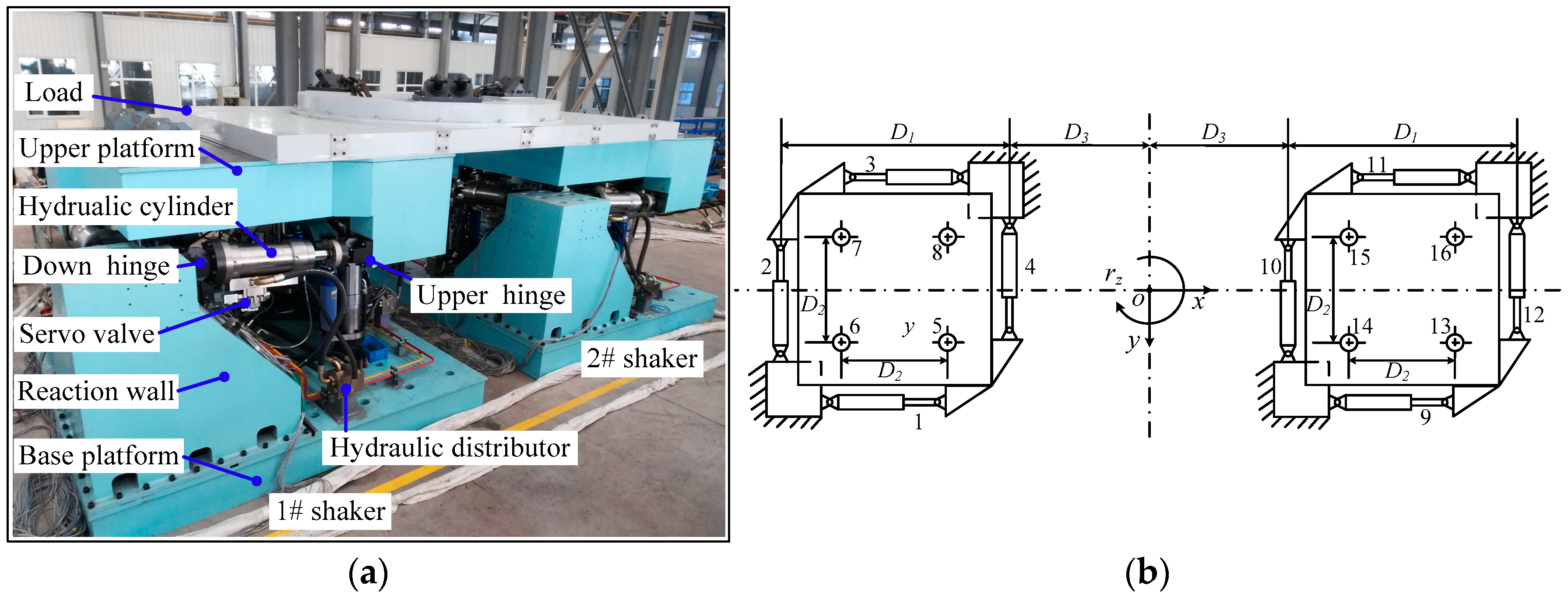
The dual-shaking table system has two identical electro-hydraulic shaking tables, as shown in Figure 1. Each shaking table is composed of an upper platform (table), two reaction walls, 16 spherical hinges, a base platform and eight hydraulic actuators: two for X direction, two for Y direction and four for Z direction, as shown in Figure 1b.

The actuators are controlled by three-stage electro-hydraulic servo valves. Each actuator is equipped with a linear variable differential transformer (LVDT) displacement sensor to measure the displacement of the piston rod, an acceleration sensor fixed on the platform as close as to the piston rod as possible and two pressure sensors, which are used to measure the pressures of the upper and down cavity of hydraulic cylinder. Each shaking table can realize six-DOF motions: three translations along X, Y and Z axes and three rotations around X, Y and Z axes.

The characteristics of the load are very important to the shaking table system performance. They not only affect the control performance of the individual shaking table, but also affect the control performance of the other shaking table due to the coupling action of the load. The stiffness of the load affects the coupling action and the eccentricity of the load mass affects the synchronization control precision. If the stiffness of the load and the eccentricity of the load mass are relatively large, the coupling action between the tables is strong and the synchronization error is large, which will make the control of the shaking table more difficult and vice versa. However, because the main research scope of this paper is the control of the tables and is not the research of the specimen’s response performance and an experiment specimen is very expensive to build, so this paper uses a simple specimen with relatively high stiffness to verify the proposed control strategy in the later experiment verification section.

The large-span test specimen is fixed on two tables, which provide synchronous motions to test the anti-seismic performance of the specimen. The specimen is a relatively stiff specimen and will be used in the following experimental validation tests in Section 4 of this paper. The size of the specimen is 7.5 m × 2.5 m × 0.3 m and the mass of the specimen is 6 t. The specimen is composed of two floors of steel plates through welding and there is a cylinder about 0.2 m height connected with it through welding. The mass of the cylinder is about 300 kg and the diameter is about 2 m. The main specific system parameters are listed in

Table 1. Main parameters of dual-shaking table system.

Parameters	Values Units
Size of the platform	2.5 m × 2.5 m
Maximum mass of load	10 t
Maximum displacement	±0.125(X/Y), ±0.1(Z) m
Maximum velocity	±0.5 m/s
Maximum acceleration	2.0 g
Frequency width of system	0.1~50 Hz
D1/D2/D3 in Figure 1b	2.547/1.55/2.7 m

. Note that the two shaking tables will share the total mass of the load, but the mass will not surely be halved as this is due to the possible eccentricity of the load mass, which is one of the factors causing the differing dynamic performance of the two shaking tables.

2.2. Hydraulic Cylinder Design

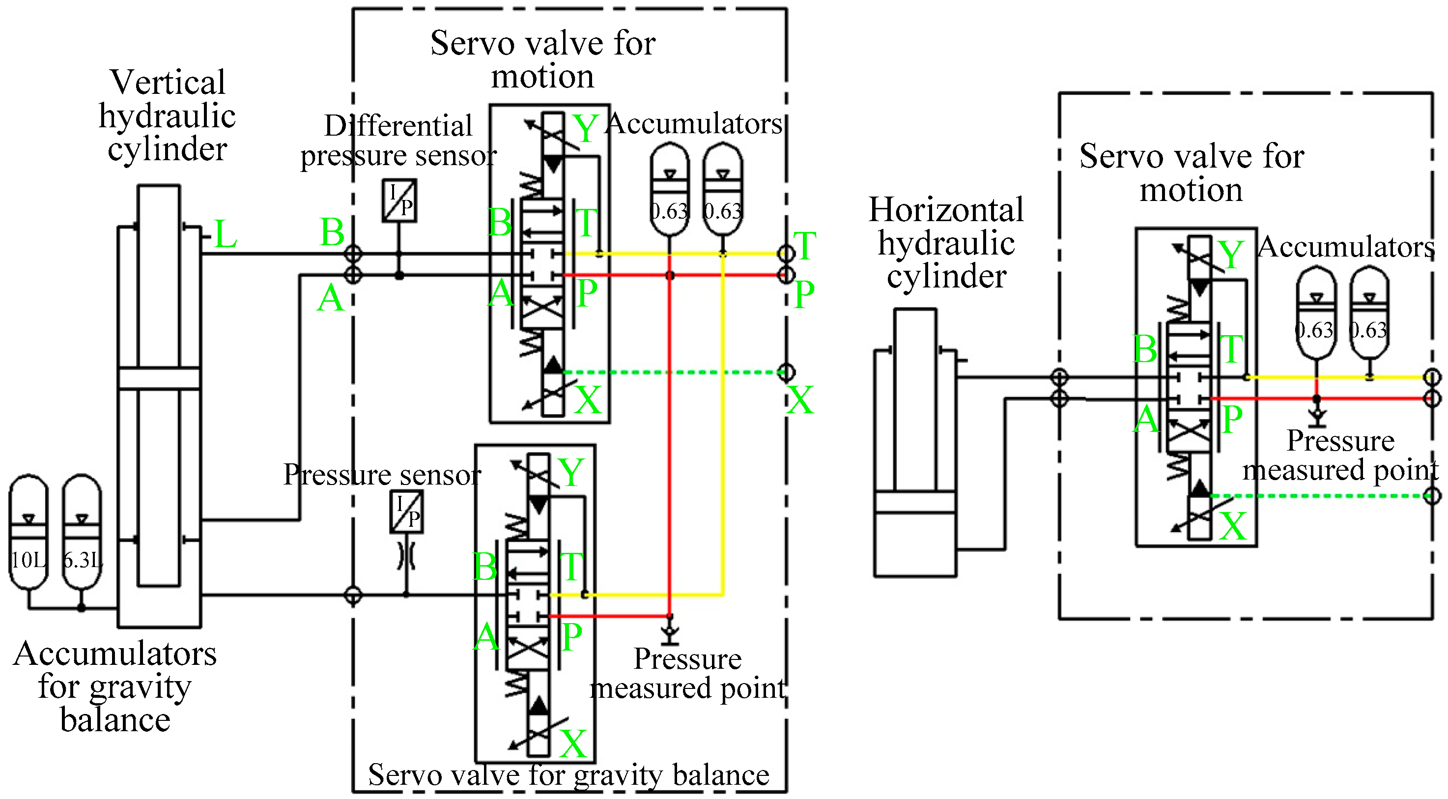
Hydraulic cylinders are the actuators of the hydraulic system, as is shown in Figure 1. Figure 2 shows the hydraulic principle diagram of the horizontal and vertical valve-controlled hydraulic cylinders, respectively. The motion of shaking tables has the characteristics of high frequency and small displacement amplitude. So, to reduce the friction and wear and prolong the lifespan of hydraulic cylinder, the clearance seal technique [34,35] is adopted. Note that the horizontal hydraulic cylinders are designed as asymmetric to save space.

For each horizontal hydraulic cylinder, with the maximum acceleration 2 g shown in Table 1, the maximum dynamic force is derived as

$$F_{x,y}=\left(\frac{m_0}{2}+\frac{m}{2}\right)\times a=1.47\times {10}^5\mathrm{N}$$

(1)

where, m₀ is the mass of the table, m₀ = 5 t; m is the mass of maximum load, m = 10 t; a is the maximum acceleration, a = 2 g.

To ensure the system performance, we define 80% of the maximum static force of hydraulic cylinder as the maximum dynamic force, so the effective area of the hydraulic cylinder is

$$A_{x,y}=\frac{5F_{x,y}}{4P_s}=73.5 {\text{cm}}^2$$

(2)

where, P_s is the hydraulic power supply pressure, P_s = 25 MPa.

In order to round the diameters, according to the hydraulic design handbook [36], the diameters of piston rod and piston are chosen as 100 mm/140 mm, which has a close effective area to the computed value in Equation (2). Consequently, the maximum static thrust/drawing forces of horizontal hydraulic cylinder designed are 384 kN/188.5 kN. The maximum dynamic thrust/drawing forces are 307 kN/150.8 kN.

Similarly, for the vertical hydraulic cylinder, the maximum force is

$$F_z=\left(\frac{m_0}{4}+\frac{m}{4}\right)\times a+\frac{M}{4D_2}=1.22\times {10}^5\mathrm{N}$$

(3)

where, M is the maximum overturning moment, M = 150 kN·m.

The diameters of the piston rod and piston are 100 mm/140 mm. The maximum static/dynamic forces are 188.5 kN/150.8 kN.

2.3. Electro-Hydraulic Servo Valve Design

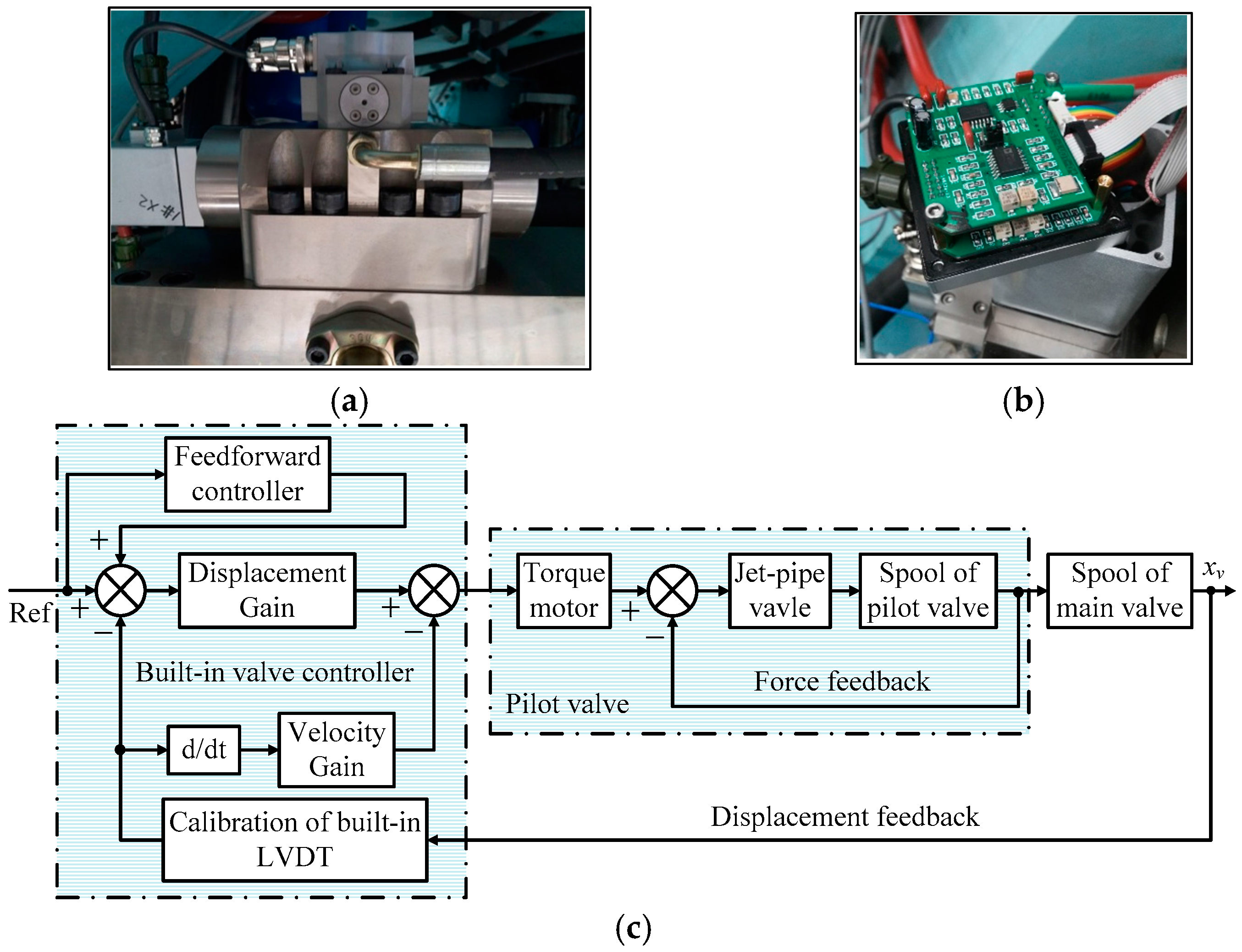
For shaking tables system, the servo valves need to have good dynamic and static performance and consistency, especially for the redundant-driven shaking table. The performance of the commercially available servo valve is fixed and it often has poor consistency, which is the main reason causing the differing performances of valve-controlled hydraulic cylinders. To solve this problem, the three-stage electro-hydraulic servo valve [37] with parameter-tunable valve controller is developed, as shown in Figure 3. The servo valve is mainly composed of four parts: pilot valve, built-in valve controller, main valve and built-in linear variable differential transformer (LVDT) to measure the displacement of the main valve. Also, the built-in valve controller has several tunable parameter gains, such as feedback gain, velocity gain and feed-forward gain, etc. to adjust the performance of the servo valve. The basic hydraulic and control schematic is shown in Figure 3c.

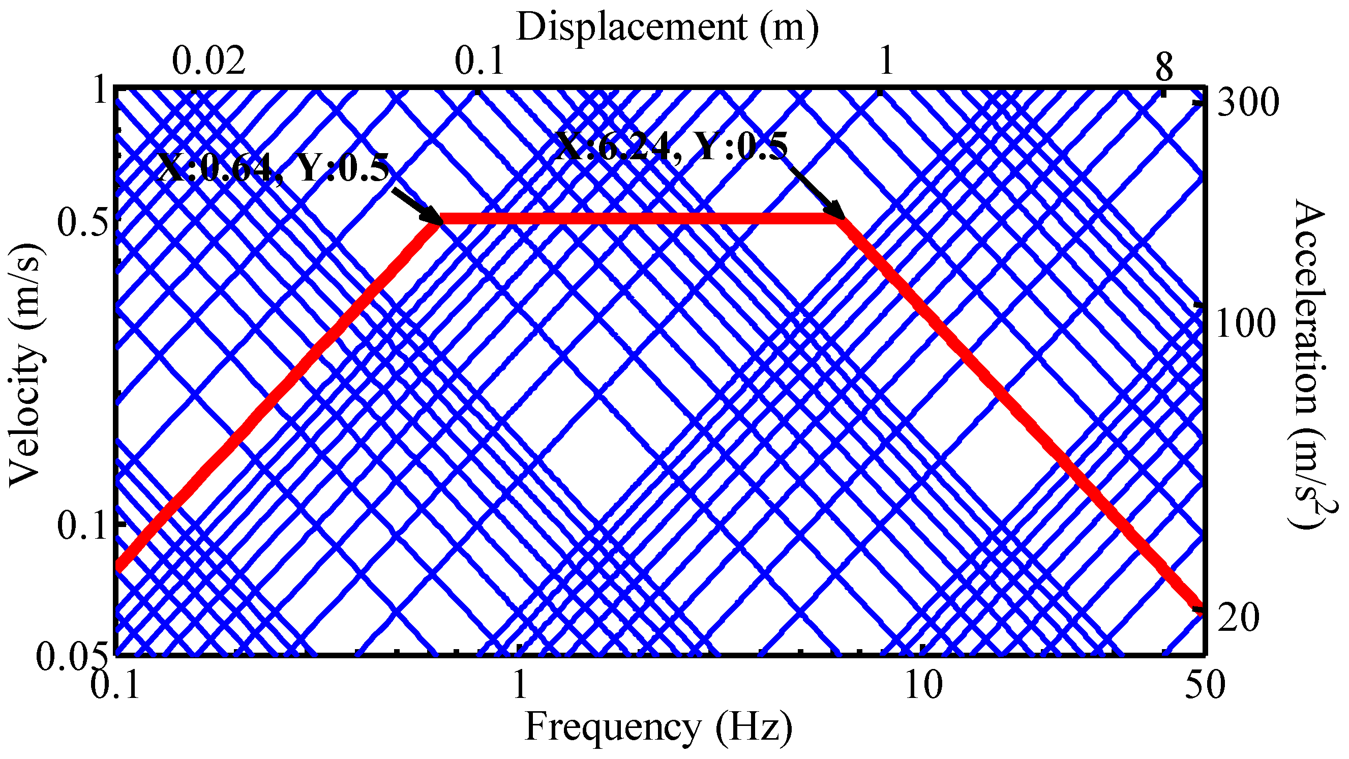
For the horizontal servo valve, the maximum velocity is 0.5 m/s, so the maximum flow is

$$Q_{x,y}=A_{x,y}^d{v}_{x,y}=\frac{\mathsf{\pi }}{4}{D}^2{v}_{x,y}=462 \mathrm{L}/\min$$

(4)

where, D is the diameter of the horizontal cylinder piston.

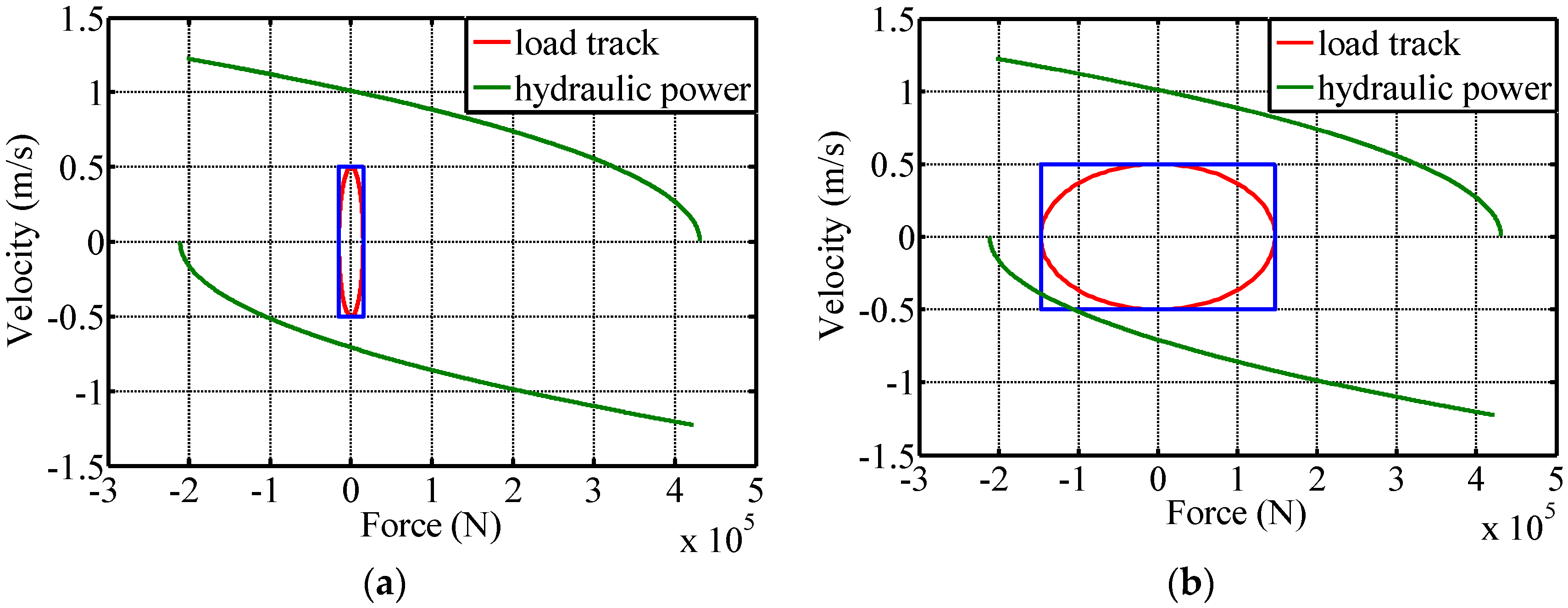
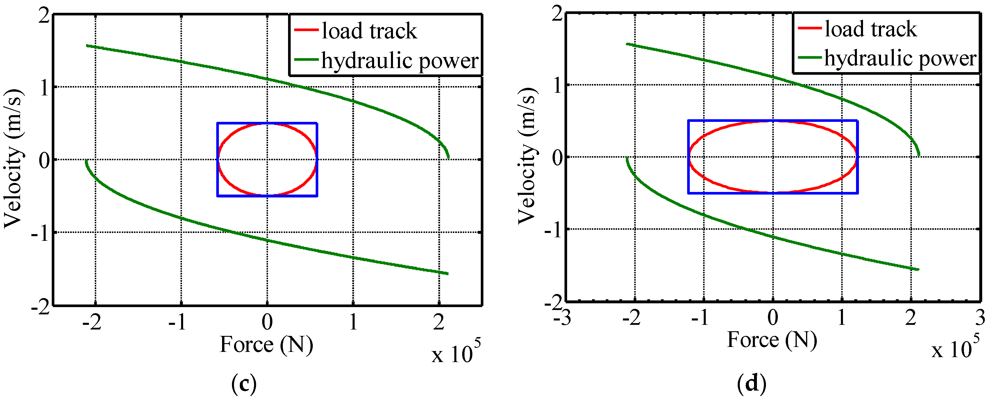
Figure 4 shows the maximum capability curve of the shaking tables system, which indicates the relationship between frequency and maximum displacement, velocity and acceleration. The computed servo valve flow in Equation (4) is at the point where the maximum velocity and maximum force occur simultaneously. However, for the shaking table system, whose main force is the inertia force, the maximum acceleration and the maximum velocity cannot be reached at the same time; that is to say, the maximum force and maximum velocity cannot be reached simultaneously. For hydraulic power, the needed flow becomes smaller with the increased force needed and vice versa. So, the hydraulic power does not need the maximum flow 462 L/min at the maximum force moment. Considering Equation (4), we choose the optimal rated flow of horizontal servo valve as 400 L/min. The optimal load matching curves using the 400 L/min valve corresponding to the turning points of Figure 4 are shown in Figure 5a,b, which indicate that the chosen valve can meet the maximum flow requirement with certain allowance to ensure the system performance [38]. The rectangle around the load track curves in Figure 5 is the curve, whose four corner points are the assumptive load track points with the maximum force and maximum velocity simultaneously. Also, the four points provide reference during the design process of the hydraulic power. Besides, the horizontal servo valve is designed as asymmetric to match the asymmetric horizontal hydraulic cylinder.

For the vertical servo valve, the design process is similar and the rated flow is chosen as 250 L/min. The optimal load matching curves using the 250 L/min valve at turning points of Figure 4 are shown in Figure 5c,d. Furthermore, the servo valve is designed as symmetric to match the symmetric vertical hydraulic cylinder.

Furthermore, to ensure the consistency and performance, the designed valve controller has several tunable parameters, which contain the offset of pilot valve, the offset of main valve spool, displacement feedback gain, velocity feedback gain and feed-forward gain. By tuning these parameters, the servo valves can have approximately identical performances.

2.4. Gravity Balance System Design

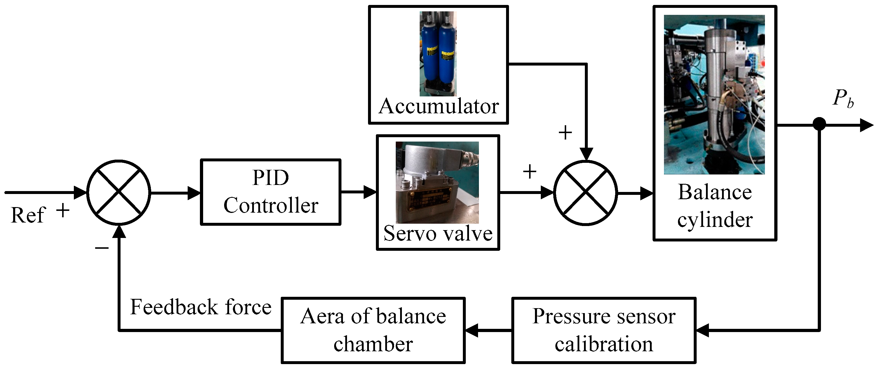
To reduce output forces of vertical hydraulic cylinders and eliminate the gravity influence of platform and load, the gravity balance system [39,40] is proposed. The gravity balance system is added to the vertical hydraulic cylinder in series. As is shown in Figure 6, the gravity balance system is a forced close-loop control system. The pressure sensor measures the pressure of the balance chamber; the error of the given force and feedback force is adjusted through the controller, and then the adjusted signal is sent to servo valve to control the output force of balance chamber. Note that the accumulator in Figure 6 is used to assist the servo valve to control the pressure due to fast response performance and good absorption of the pressure fluctuation.

The response speed of the servo valve is restricted by the frequency width, while the response speed of the accumulator is very fast. So, the balance system is controlled by the servo valve assisted by the accumulators group, which can balance the gravity more quickly. When the shaking tables are static, the gravity balance system is mainly controlled by the valve-controlled force close-loop system and when the shaking tables move, the gravity balance system is mainly controlled by accumulators group.

The accumulators group is composed of two different accumulators: one is pre-charged with low pressure only to balance the mass of the table and the other is pre-charged with high pressure to balance the mass of the table and load.

The minimum balance pressure of each hydraulic cylinder is

$$F_{b\min }=\frac{m_{0}g}{4A_b}=\frac{m_{0}g}{\mathsf{\pi }{d}^2}=1.56 \text{MPa}$$

(5)

where A_b is the effective area of the balance chamber.

The maximum balance pressure of each hydraulic cylinder is

$$F_{b\max }=\frac{(m_0+m)g}{4A_b}=\frac{(m_0+m)g}{\mathsf{\pi }{d}^2}=4.68 \text{MPa}$$

(6)

The working pressure of the first stage accumulator is 1.56 Mpa in Equation (5). To keep the balance force stable, the pressure fluctuation is chosen as less than 12%, that is from P_1min = 1.373 MPa to P_1max = 1.747 MPa.

The maximum volume change of the accumulator is

$$V_{b\max }=A_{b}l=1.57 \mathrm{L}$$

(7)

where l is the maximum displacement of the vertical hydraulic cylinder, l = 200mm, as shown in Table 1.

In this condition, the accumulator is used to compensate the oil leakage and pressure loss. Thus, the velocity of the accumulator to charge and drain oil is slow, then the volume can be computed according to the isothermal formula. Combining Equation (7), the volume of the accumulator can be obtained [41]

$$V_{b1}=\left(\frac{P_{1\min }}{P_{10}}\right)\left(\frac{P_{1\max }}{P_{1\max }-P_{1\min }}\right)V_{b\max }=8.63 \mathrm{L}$$

(8)

where P₁₀ is the pre-charged pressure, P₁₀ = 0.85P_1min.

So, we choose the volume of the first stage accumulator as V_b1t = 10 L.

The design process of the second-stage accumulator is similar to the first one, so the detailed process is not introduced here and the volume of the second-stage accumulator is chosen as V_b2t = 6.3 L.

As we all know, the shaking tables have by default a built-in design limitation, which needs the effective compensation of rocking. Due to the structural limitation of the shaking table, the original point of the shaking table’s control system cannot be at the point of the center of the mass. As a consequence, when the shaking table and load move in the translational direction, the reaction force of the load will cause the rocking of the shaking table and load in the rotational direction simultaneously. To reduce the rocking of the shaking table and load, the effective compensation control of the rocking is generally added to the control system. Many references [42,43,44] have studied this problem. Seki [42] proposed two degrees of freedom control strategy based on a feed-forward controller and feedback controller to suppress this phenomenon and later he [43] proposed an adaptive notch filter to solve this problem. Dozono [44] studied the adaptive filter in order to compensate the disturbance of the reaction force caused by the specimen. As this is not the main scope of this paper, it will not be discussed in detail in this paper.

2.5. Hydraulic Power Supply Design

For the hydraulic power supply of shaking tables, the flow and its change range is large [41,44]. So, to reduce the cost, the hydraulic power flow is supplied by the hydraulic pump cooperating with the accumulators group, which is taken as the assistant hydraulic power supply. The average flow is supplied by the hydraulic pump and the flow exceeding the average flow is supplied by the accumulators group.

The shaking tables system is mainly used to perform earthquake simulation tests, so the flow of hydraulic power supply is usually designed according to El-Centro acceleration waveform, which is a typical earthquake waveform recording a strong earthquake. In the reference [40], the suggested flow of the hydraulic power supply for the shaking table system is 0.1Q_max, which is the statistical calculation result of the three typical earthquake waveforms: El-Centro, San-Fornando and Parfield. 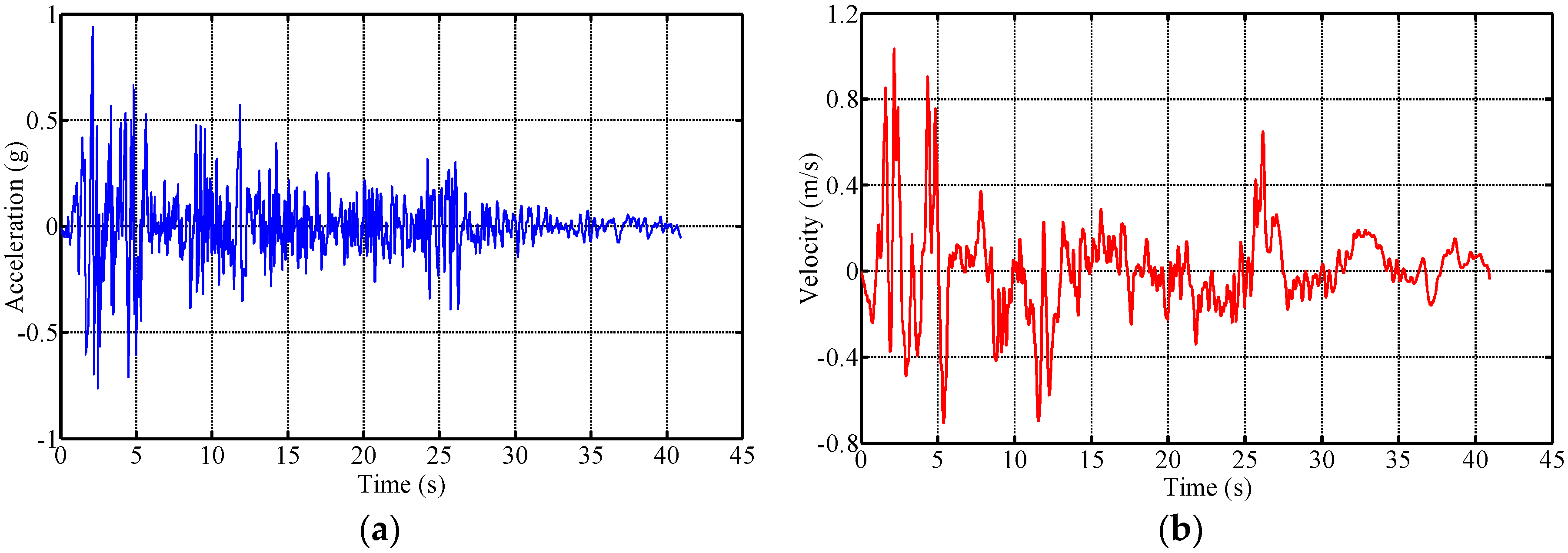For the shaking table system researched in this paper, the flow 0.1Q_max is only about 260 L/min, which is relatively small and only considers the earthquake waveform experiment. The needed flow for the El-Centro waveform is a half of the flow for the uniform random waveform. So, for more common use in the uniform random waveform experiment, this paper designed the flow according to the El-Centro earthquake waveform, whose maximum velocity is twice the required one in Table 1. Note that the design of the flow only uses the waveform of the El-Centro, the quantity of the maximum velocity is based on the requirement of the system. The El-Centro acceleration and velocity waveforms are shown in Figure 7a,b.

Then, the average flow of the horizontal hydraulic cylinder can be obtained

$$\overline{Q}=\frac{{\displaystyle {\int }_0^T{Q}_h(t)dt}}{T}=\frac{{\displaystyle {\int }_0^T|A_{x,y}\cdot {\displaystyle {\int }_0^{t}a(t)\cdot dt}|dt}}{T}$$

(9)

where, T is the total time of El-Centro waveform, a(t) is El-Centro acceleration waveform.

According to Equation (9), we can obtain the total average flow as

$$\overline{Q_t}=2{\overline{Q}}_x+2{\overline{Q}}_y+4{\overline{Q}}_z=458 \text{L}/\text{min}$$

(10)

Considering the oil supply of pilot valve, we choose the flow supplied by the hydraulic pump as Q_B = 500 L/min for each shaking table.

The working volume of the accumulators group at time t is

$$V_w(t)={\displaystyle {\int }_0^t\left(Q_h(t)-Q_B\right)}\cdot dt={\displaystyle {\int }_0^t\left(|A_{x,y}\cdot {\displaystyle {\int }_0^{t}a(t)\cdot dt}|-Q_B\right)}\cdot dt$$

(11)

The maximum change of V_w(t) is the needed working volume of the accumulators group. From Equation (11), the maximum total change V_wc for horizontal and vertical V_w(t) is

$$V_{wc}=4V_{wch}+4V_{wcv}=63.6 \mathrm{L}$$

(12)

In this case, the accumulators group is used as the assistant hydraulic power supply, so the velocity of the accumulator to charge and drain oil is very fast, and the volume change can be computed according to the adiabatic formula. Combined with Equation (12), the volume of the accumulators group is [41]

$$V=\frac{V_{wc}{\left(p_{h1}/p_{h0}\right)}^{\raisebox{1ex}{$1$}\!\left/ \!\raisebox{-1ex}{$n$}\right.}}{1-{\left(p_{h1}/p_{h2}\right)}^{\raisebox{1ex}{$1$}\!\left/ \!\raisebox{-1ex}{$n$}\right.}}=506.2 \mathrm{L}$$

(13)

where P_h1 is the minimum working pressure, P_h1 = 0.8P_h2; P_h2 is the maximum working pressure, P_h2 = P_s; P_h0 is the pre-charged pressure, P_h0 = 0.8P_h1 and n = 1.4.

In conclusion, the flow of the hydraulic power supply of the shaking tables system supplied by the hydraulic pump is 1000 L/min and the volume of the accumulators group is 1000 L.

3. Control Scheme Design

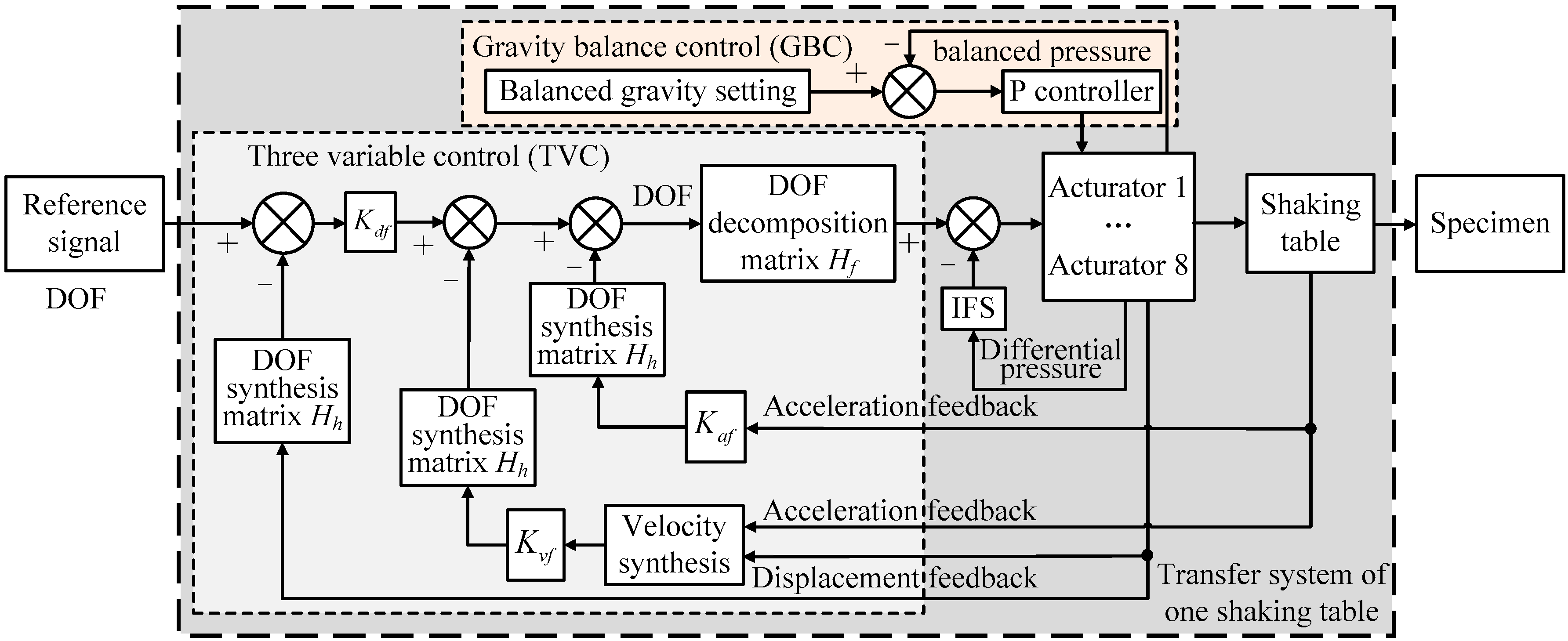
Figure 8 shows the fundamental control scheme of one shaking table, which consists of the DOF synthesis matrix H_h, DOF decomposition matrix H_f, traditional TVC, IFS and GBC control. The control scheme is based on the displacement DOF close-loop using the H_h and H_f, which can transfer the control and feedback signals between actuator space and DOF space [18]. TVC controller is used to improve the shaking table system performance using the acceleration, velocity and displacement feedback signals and has been successfully applied in many practical shaking table systems [19,21,45]. The gravity balance control is relatively simple, and the force closed-loop control is used for each balanced hydraulic cylinder, whose controller is a proportion controller. To reduce the inner force of the redundant-driven shaking table system due to the inconsistencies of the valve-controlled hydraulic cylinders’ performances, the IFS is proposed by Plummer and Wei and obtained a better suppression effect [18,20]. Therefore, to improve the system performance, this paper applies the TVC and IFS as the fundamental control scheme for the platform motion control system, as shown in Figure 8. Note that the velocity signal is synthesized using the acceleration and displacement in practice.

Generally, the experiment specimen of the shaking table is the civil engineering structure, which is mostly reinforced concrete structure [5,6]. As we all know, the reinforced concrete structure specimen is easily damaged when the specimen encounters large deformation. If the attitude control errors of the shaking tables are large, especially one or both of the shaking tables lose control due to misoperation, which will cause significant deformation to the specimen, even damage. Thus, the synchronization control strategy is needed first to reduce the undesired synchronization error of the shaking tables to avoid the large deformation of the specimen. The synchronization control will keep the shaking tables moving synchronously even though there is large attitude control error or it is out of control. Based on the synchronization control, the tracking control precision also needs to be ensured, thus the feed-forward inverse model is adopted, which has many advantages, such as being independent of the system’s stability. However, the identified model errors, designed inverse model errors and some disturbance can still affect the tracking control precision. 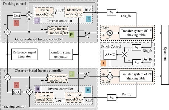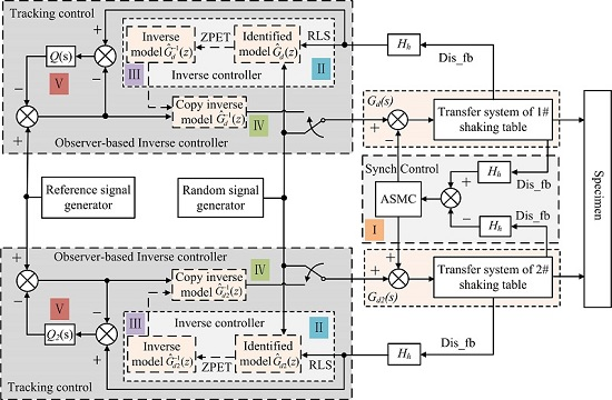To improve the control precision further, the disturbance-observer feed-forward inverse model is proposed based on synchronization control, as shown in Figure 9.

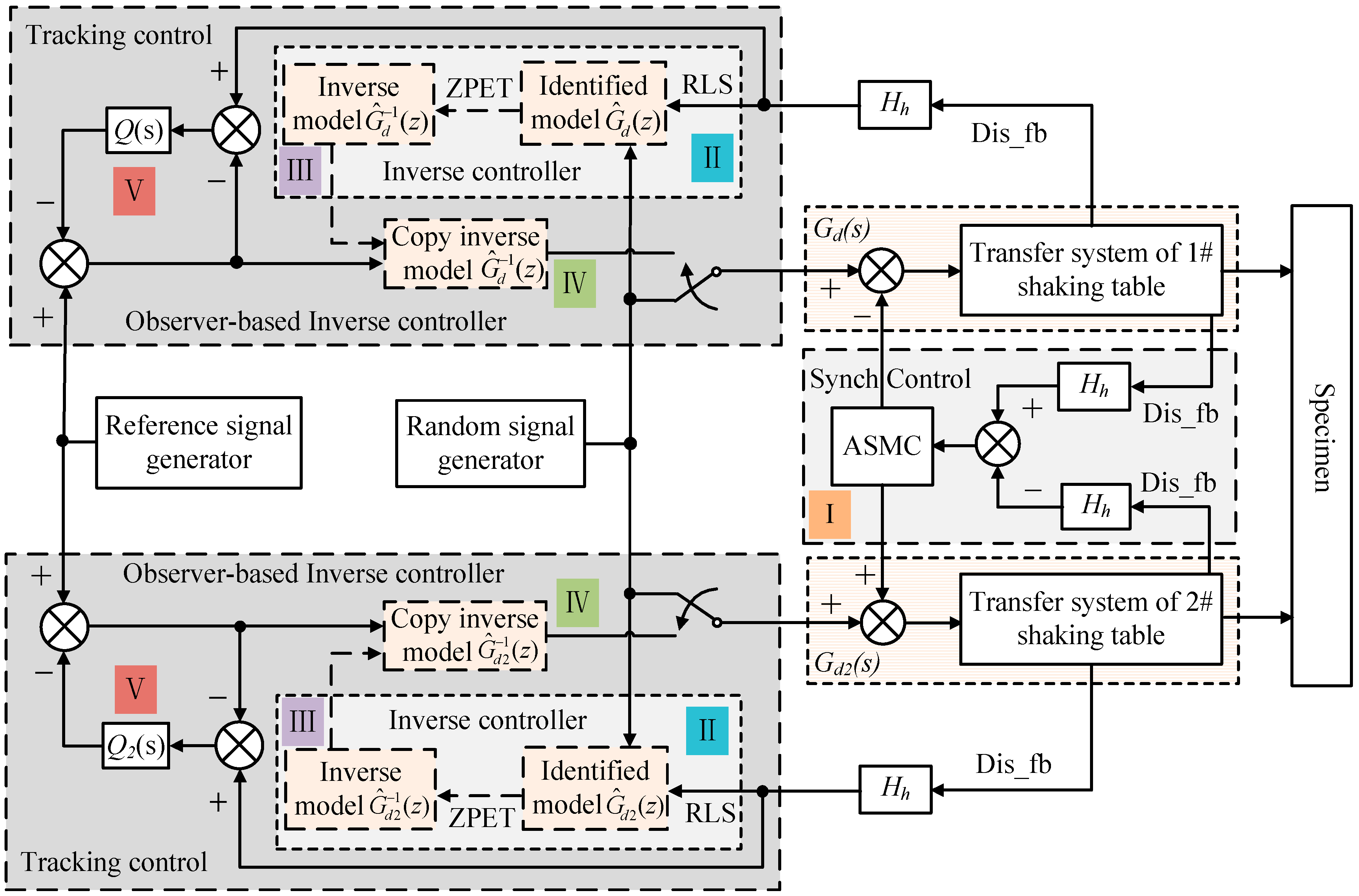
Figure 9 shows the proposed control scheme of the dual-shaking table system. As is shown in the figure, the control system mainly contains the fundamental displacement DOF close-loop control based on Figure 8, synchronization control and tracking control. The cross-coupled synchronization controller ASMC, which can adaptively tune the parameters of the SMC, is proposed to reduce the synchronization error of two shaking tables though compensation control of error to the reference input port of the fundamental close-loop control. On that basis, the feed-forward observer-based inverse model controller combining the inverse model controller and disturbance observer is used to improve the tracking control performance. The proposed compound controller has the advantages of inverse controller and disturbance observer and has a high tracking precision. As can be seen in the figure, the ASMC synchronization controller and observer-based inverse model controller act as an outer control loop of the fundamental close-loop control. Note that this paper mainly studies the synchronization and tracking control, which prefers to obtain the same response performance under the same reference signal, so in the control system the same one reference signal is given to the two shaking tables.

Because this paper mainly studies the synchronization and tracking control of the shaking tables, in which the coupling effect of the specimen on each shaking table is regarded as a disturbance of each shaking table. For considering the problem in this paper, the main difference between the flexible and stiff specimens is the different value of the disturbance, so the control strategy will be applicable to both the flexible and stiff specimens and has a strong robustness to the behavior of the specimen. For the specimens with different stiffness, the main difference to the control strategy is the values of the control parameter gains. Furthermore, the disturbance influence of the high stiffness specimen is larger than the low stiffness one, thus if the control strategy is verified with the high stiffness specimen in the later experiment tests, then the control strategy should be correct and feasible with low stiffness specimen, theoretically. However, due to the condition restriction, the test specimen is very expensive and time-consuming to build, so this paper cannot perform the validation tests with a flexible specimen now, and will be tested later when the test specimen is provided.

As shown in Figure 9, there are five main steps to realizing the proposed control scheme of the dual-shaking table, as follows:

(1)

Synchronization control: the reference signal (random or step signal) is given to the transfer systems of two shaking tables without observer-based inverse model controller acting. The parameters of AMSC are tuned to reduce the synchronization error until it stops reducing.

(2)

System identification: The random signal is given to the dual-shaking table system with ASMC synchronization controller. The discretization transfer functions ${\widehat{G}}_d(z)$ and ${\widehat{G}}_{d2}(z)$ of the system are identified online based on the RLS algorithm.

(3)

Inverse controller design: The inverse model controllers ${\widehat{G}}_d^{-1}(z)$ and ${\widehat{G}}_{d2}^{-1}(z)$ are designed based on the identified transfer functions and ZPETC technique.

(4)

Copy inverse model controller: the designed inverse controller ${\widehat{G}}_d^{-1}(z)$ and ${\widehat{G}}_{d2}^{-1}(z)$ are copied into the transfer system as the feed-forward controller.

(5)

Observer-based inverse model controller: the low-filters Q(s) and Q₂(s) of the disturbance observer are put into the control system cooperating with the inverse controller.

3.1. Synchronization Controller Design

To obtain a satisfactory synchronization control precision of dual-shaking table system, this paper proposes a novel ASMC based on adaptive reaching law to cross-coupling control strategy, as is shown in Figure 9. The attitude DOF control signal is compensated by the synchronization control signal, which is processed by the proposed ASMC synchronization controller according to the attitude feedback error of two shaking tables. For convenience, we define the left shaking table in Figure 1b as 1# shaking table and the right one as 2# shaking table, and use subscript i to represent the ith table in the following parts, i = 1,2.

The attitude tracking error, velocity tracking error and acceleration tracking error of each shaking table can be defined as

$$\begin{array}{l}{\mathit{q}}_{ie}={\mathit{q}}_{ir}-{\mathit{q}}_i\\ {\dot{\mathit{q}}}_{ie}={\dot{\mathit{q}}}_{ir}-{\dot{\mathit{q}}}_i\\ {\ddot{\mathit{q}}}_{ie}={\ddot{\mathit{q}}}_{ir}-{\ddot{\mathit{q}}}_i\end{array}$$

(14)

where ${\mathit{q}}_{ir}$ is the reference attitude (DOF) signal, ${\mathit{q}}_i$ is the feedback attitude signal and there is ${\mathit{q}}_{1r}={\mathit{q}}_{2r}={\mathit{q}}_r$.

The attitude synchronization error, velocity synchronization error and acceleration synchronization error can be defined as

$$\begin{array}{l}{\mathit{q}}_{ise}={(-1)}^i({\mathit{q}}_2-{\mathit{q}}_1)\\ {\dot{\mathit{q}}}_{ise}={(-1)}^i({\dot{\mathit{q}}}_2-{\dot{\mathit{q}}}_1)\\ {\ddot{\mathit{q}}}_{ise}={(-1)}^i({\ddot{\mathit{q}}}_2-{\ddot{\mathit{q}}}_1)\end{array}$$

(15)

The synchronization control sliding mode surface is designed as

$${\mathit{s}}_{is}(t)={\left(\frac{d}{dt}+{\mathit{\lambda }}_i\right)}^2{\mathit{q}}_{ise}={\ddot{\mathit{q}}}_{ise}+{\mathit{c}}_{i2}{\dot{\mathit{q}}}_{ise}+{\mathit{c}}_{i1}{\mathit{q}}_{ise}$$

(16)

Using the exponential reaching law to design the control law can not only improve the dynamic quality of the reaching phase of the sliding mode, but also reduce the system chattering by choosing the appropriate reaching law parameters [46]. So, this paper applies the SMC based on exponential reaching law. The traditional exponential reaching law is

$${\dot{\mathit{s}}}_{is}(t)=-\mathit{k}{\mathit{s}}_{is}-\mathsf{\beta }sign({\mathit{s}}_{is})$$

(17)

where, ${\mathit{k}}_{s6\times 6}$ and ${\mathsf{\beta }}_{s6\times 6}$ are the diagonal matrixes with positive constants.

This reaching law can be divided into two parts: ${\dot{\mathit{s}}}_{is}=-{\mathit{k}}_s{\mathit{s}}_{is}$ is the exponential reaching part, whose solution is ${\mathit{s}}_{is}={\mathit{s}}_{is}(0)e^{-kt}$, and ${\dot{\mathit{s}}}_{is}=-{\mathsf{\beta }}_{s}sign({\mathit{s}}_{is})$ is the constant speed reaching part. As the coefficient matrixes ${\mathit{k}}_s$ and ${\mathsf{\beta }}_s$ are constant matrixes, the system does not have the ability of adaptive tuning. So, for different system state variables, the convergence performance cannot achieve the optimal effect. To solve this problem, this paper proposes an adaptive variable speed reaching law

$${\dot{\mathit{s}}}_{is}(t)=-{\mathit{k}}_s(1+c{\Vert {\mathit{s}}_{is}\Vert }^{1/\mathsf{\gamma }}){\mathit{s}}_{is}-{\mathsf{\beta }}_s(1+{\Vert {\mathit{s}}_{is}\Vert }^{\mathsf{\gamma }}/c)sign({\mathit{s}}_{is})$$

(18)

where, $c$ and $\mathsf{\gamma }$ are positive constants, and $0<\mathsf{\gamma }<1$.

The proposed reaching law can tune the reaching speed adaptively according to the distance between the system state variables and the sliding mode surface. When the system state is far away from the sliding mode surface, $\Vert {\mathit{s}}_{is}\Vert$ is quite large and the reaching law can be approximated to ${\dot{\mathit{s}}}_{is}(t)=-{\mathit{k}}_s(1+c{\Vert {\mathit{s}}_{is}\Vert }^{1/\mathsf{\gamma }}){\mathit{s}}_{is}$, which has a far higher speed compared with the traditional exponential reaching law and can largely reduce the reaching time. When the system state variables point is close to the sliding mode surface, $\Vert {\mathit{s}}_{is}\Vert$ is quite small and the reaching law can be approximated to ${\dot{\mathit{s}}}_{is}=-{\mathsf{\beta }}_s(1+{\Vert {\mathit{s}}_{is}\Vert }^{\mathsf{\gamma }}/c)sign({\mathit{s}}_{is})$, which can reduce the system chattering by increasing the gain $\gamma$ and decreasing the gain $c$. When $\Vert {\mathit{s}}_{is}\Vert$ is close to zero, the adaptive reaching law degrades into the traditional exponential reaching law.

The sliding mode synchronization control law is designed as follows

$${\mathit{u}}_{ise}(t)=-\left[{\mathit{k}}_s(1+\mathsf{\epsilon }{\Vert {\mathit{s}}_{is}\Vert }^{1/\mathsf{\tau }}){\mathit{s}}_{is}+{\mathsf{\beta }}_s(1+{\Vert {\mathit{s}}_{is}\Vert }^{\mathsf{\tau }}/\mathsf{\epsilon })sign({\mathit{s}}_{is})\right]$$

(19)

where, ${\mathit{k}}_{s(6\times 6)}$ and ${\mathsf{\beta }}_{s(6\times 6)}$ are diagonal matrixes with positive constants. The constant gains $\mathsf{\epsilon }>0$ and $0<\mathsf{\tau }<1$.

3.2. Model Inverse Controller Design

As is shown in Figure 9, in the proposed control scheme, the control of each shaking table is a displacement DOF close-loop system and the proposed ASMC is used to reduce the synchronization error of dual shaking tables through the cross-coupled compensation control. With synchronization control, the performances of the two shaking tables are very similar, and the coupling effect of the specimen on each shaking table control system due to the synchronization error is considered as disturbance. This section is aimed to improve the tracking performance of each shaking table displacement close-loop system through the outer loop controller using the proposed observer-based inverse model controller. So, for each shaking table, the tracking control scheme is the same. Thus, the following parts introduce the tracking control scheme for only one shaking table for simplicity, and it is applicable to the other one.

In this section, the RLS algorithm is applied to identify the system close-loop transfer function, which will be used to design the system inverse model controller. The RLS algorithm is referred in Eweda [30]. We define that the discretization transfer function of 1# shaking table close-loop system G_d(s) is G_d(z), then the auto regressive moving model of G(z) can be described as

$$A(z^{-1})y(t)=B(z^{-1})u(t-d)+\mathsf{\xi }(t)$$

(20)

where, y(t) is the system output sequences and there is $A(z^{-1})=1+a_1{z}^{-1}+\mathrm{...}+a_n{z}^{-n}$; u(t) is the system input sequences and there is $B(z^{-1})=b_0+b_1{z}^{-1}+\mathrm{...}+b_m{z}^{-m}$ and ξ(t) is a random white noise sequence with zero mean.

Writing Equation (20) into least squares form gives

$$y(t)=\widehat{\mathsf{\phi }}(t)\mathsf{\theta }+\mathsf{\xi }(t)$$

(21)

where $\mathsf{\phi }(t)=[-y(t-1),\mathrm{...},-y(t-n),u(t-d),\mathrm{...},-u(t-d-m)]$, $\mathsf{\theta }=[a_1,\mathrm{...},a_n,b_0,\mathrm{...},b_m]$.

The noise signal ξ(t) as the estimator can be written as

$$\widehat{\mathsf{\xi }}(t)=y(t)-\widehat{y}(t)=y(t)-{\widehat{\mathsf{\phi }}}^T(t)\widehat{\mathsf{\theta }}(t)$$

(22)

where $\widehat{\mathsf{\theta }}=[{\widehat{a}}_1,\mathrm{...},{\widehat{a}}_n,{\widehat{b}}_0,\mathrm{...},{\widehat{b}}_m]$, $\widehat{\mathsf{\phi }}(t)=[-\widehat{y}(t-1),\mathrm{...},-\widehat{y}(t-n),\widehat{u}(t-d),\mathrm{...},-\widehat{u}(t-d-m)]$.

To obtain system parameters $\widehat{\mathsf{\theta }}$, the RLS algorithm employed can be put as [27]

$$\begin{array}{c}\widehat{\mathsf{\theta }}(t)=\widehat{\mathsf{\theta }}(t-1)+K(t)[y(t)-{\widehat{\mathsf{\phi }}}^T(t)\widehat{\mathsf{\theta }}(t-1)]\\ K(t)=\frac{P(t-1)\widehat{\mathsf{\phi }}(t)}{1+{\widehat{\mathsf{\phi }}}^T(t)P(t-1)\widehat{\mathsf{\phi }}(t)}\\ P(t)=[I-K(t){\widehat{\mathsf{\phi }}}^T(t)]P(t-1)\end{array}$$

(23)

Ideally, the exact system inverse model can be obtained and allows to accurately track the system’s desired trajectory. However, for the identified system model in Equation (20), there are always zeros outside the unit circle due to sampling holder, transport delay and sensors and actuators being physically non-collocated, etc. [47]. The direct inversion of the identified system model with zeros outside the unit circle is inappropriate and the system is unstable when the direct inversion is used as the feed-forward controller. To solve this problem, a stable approximate inverse model is designed instead of the exact inverse. The ZPETC proposed by Tomizuka [33] is a successfully and widely used method to design the inverse controller of the non-minimum phase system and is adopted to design the inverse controller of the identified dual-shaking table system model.

Assuming that the identified system transfer function can be expressed as

$${\widehat{G}}_d(z)=\frac{N_{+}(z)N_{-}(z)}{M(z)}$$

(24)

where $N_{+}(z)$ is factors with stable zeros, $N_{-}(z)$ is factors with unstable zeros.

The system approximate inverse model can be designed as

$${\widehat{G}}_d^{-1}(z)=\frac{M(z)N_{-}(z^{-1})}{z^p{N}_{+}(z)N_{-}^2(1)}$$

(25)

where p is the number of unstable zeros of the identified system transfer function.

The purpose of adding the term $z^p$ into Equation (25) is to ensure the designed inverse model physically realizable while ensuring the magnitude-frequency characteristic of the designed inverse model consistent with the true inverse model.

Combining Equations (24) and (25), the close-loop system transfer function with feed-forward inverse controller compensation can be obtained

$$G_s(z)={\widehat{G}}_d(z){\widehat{G}}_d^{-1}(z)=\frac{N_{-}(z^{-1})N_{-}(z)}{z^p{N}_{-}^2(1)}$$

(26)

Implementing the factorization, the $N_{-}(z)$ can be expressed as

$$N_{-}(z)={\displaystyle \prod _{i=1}^p{N}_{i-}(z)}={\displaystyle \prod _{i=1}^p(z+a_i)}\hspace{0.17em}\hspace{0.17em}|a_i|\ge 1$$

(27)

Substituting Equations (27) into (26), it can be obtained

$$G_s(z)=z^{-p}{\displaystyle \prod _{i=1}^p\frac{N_{i-}(z)N_{i-}(z^{-1})}{{\left[N_{i-}(1)\right]}^2}}=z^{-p}{\displaystyle \prod _{i=1}^p\frac{(z+a_i)(z^{-1}+a_i)}{{\left[(1+a_i)\right]}^2}}$$

(28)

Substituting z = e^jwT into Equation (28), where T is the sampling time and T = 0.001 s. Then, the following results can be obtained

$$\angle G_s(e^{jwT})=-pwT$$

(29)

$$\left|G_s(e^{jwT})\right|={\displaystyle \prod _{i=1}^p\left|\frac{a_i^2+2a_i\cos \left(\mathsf{\omega }T\right)+1}{a_i^2+2a_i+1}\right|}$$

(30)

The sampling time T is 0.001 s, thus wT can be approximately equal to 0 in a relatively large frequency width range. As a consequence, it can be obtained that $\left|G_s(e^{jwT})\right|\approx 1$ from Equation (30) and that $\angle G_s(e^{jwT})\approx 0$ from Equation (17) when wT is close to zero. From the above and combining Equations (29) with (30), it can be concluded that

$$G_s(z)={\widehat{G}}_d(z){\widehat{G}}_d^{-1}(z)\approx 1$$

(31)

The Equation (31) demonstrates that the designed ${\widehat{G}}_d^{-1}(z)$ is approximately the inverse model of the identified system model and can be used as the system feed-forward inverse controller.

3.3. Feed-Forward Inverse Control

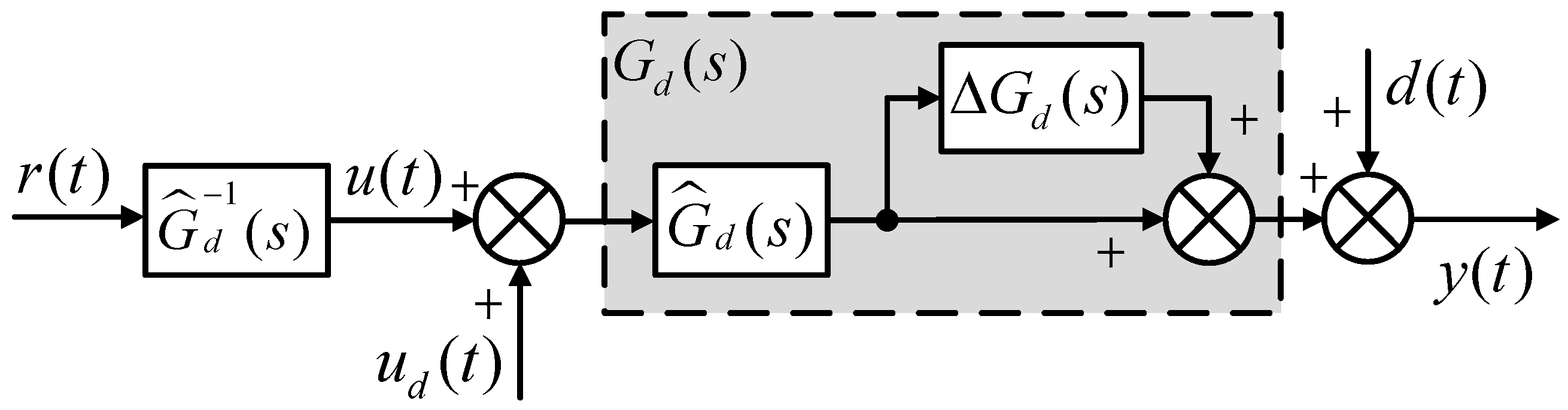
The designed inverse model controller as the feed-forward controller of the control system can improve the system control precision. However, the identified system model cannot accurately describe the actual transfer system due to the undetermined system model error with Equation (20), system nonlinearity and the RLS algorithm convergence accuracy, etc. From Equation (31), it can be seen that the designed inverse model is the only approximately inverse of the identified model. There are the system noise signals, the disturbance from the other shaking table and external disturbance, which can also affect the tracking control precision of the shaking table system.

The feed-forward inverse model controller designed in the former section is applied to the control system considering various system errors and disturbance factors, as shown in Figure 10. The $\Delta G_d(s)$ in Figure 10 is the model error between the real system model and the identified system model, u_d(t) is the cross-coupled control disturbance and d(t) is the compound disturbance, which contains the disturbance due to the specimen from the other shaking table and external disturbance source.

We define the relationship between the real system model $G_d(s)$ and the identified system model ${\widehat{G}}_d(s)$ as

$$G_d(s)={\widehat{G}}_d(s)\left[1+\Delta G_d(s)\right]$$

(32)

From Equation (31), it can be seen that the designed inverse model ${\widehat{G}}_d^{-1}(s)$ is only approximate to the real inverse model of the identified model ${\widehat{G}}_d(s)$. We define the designed system model error as $\Delta {\widehat{G}}_d(s)$ and the relationship of $\Delta {\widehat{G}}_d(s)$, ${\widehat{G}}_d^{-1}(s)$ and ${\widehat{G}}_d(s)$ is defined as

$$G_s(s)={\widehat{G}}_d(s){\widehat{G}}_d^{-1}(s)=1+\Delta {\widehat{G}}_d(s)$$

(33)

Combining Equations (32) and (33) and Figure 10, it can be obtained that

$$\begin{array}{ll}y(t)& ={\widehat{G}}_d^{-1}(s){\widehat{G}}_d(s)\left[1+\Delta G_d(s)\right]r(t)+{\widehat{G}}_d(s)\left[1+\Delta G_d(s)\right]u_d(t)+d(t)\\ & =\left[1+\Delta {\widehat{G}}_d(s)\right]\left[1+\Delta G_d(s)\right]r(t)+{\widehat{G}}_d(s)\left[1+\Delta G_d(s)\right]u_d(t)+d(t)\end{array}$$

(34)

According to Equation (34) and Figure 10, the control system error e(t) is

$$\begin{array}{ll}e(t)& =r(t)-y(t)\\ & =-\left[\Delta {\widehat{G}}_d(s)+\Delta G_d(s)+\Delta {\widehat{G}}_d(s)\Delta G_d(s)\right]r(t)-{\widehat{G}}_d(s)\left[1+\Delta G_d(s)\right]u_d(t)-d(t)\end{array}$$

(35)

When the identified system model error $\Delta G_d(s)$ and the designed system inverse model error $\Delta {\widehat{G}}_d(s)$ are both zeros, that is to say, there is no identified and designed errors with the dual-shaking table system model, then the Equation (35) becomes

$$e(t)={\widehat{G}}_d(s)u_d(t)+d(t)$$

(36)

From Equation (35), it can be seen that due to the cross-coupled effect of the two shaking tables, identified model error, the designed inverse model error and the disturbance action, the control precision of the system with feed-forward inverse controller compensation is affected. Equation (36) demonstrates that the system control error still exists even if the identified system model and designed system inverse model are completely accurate.

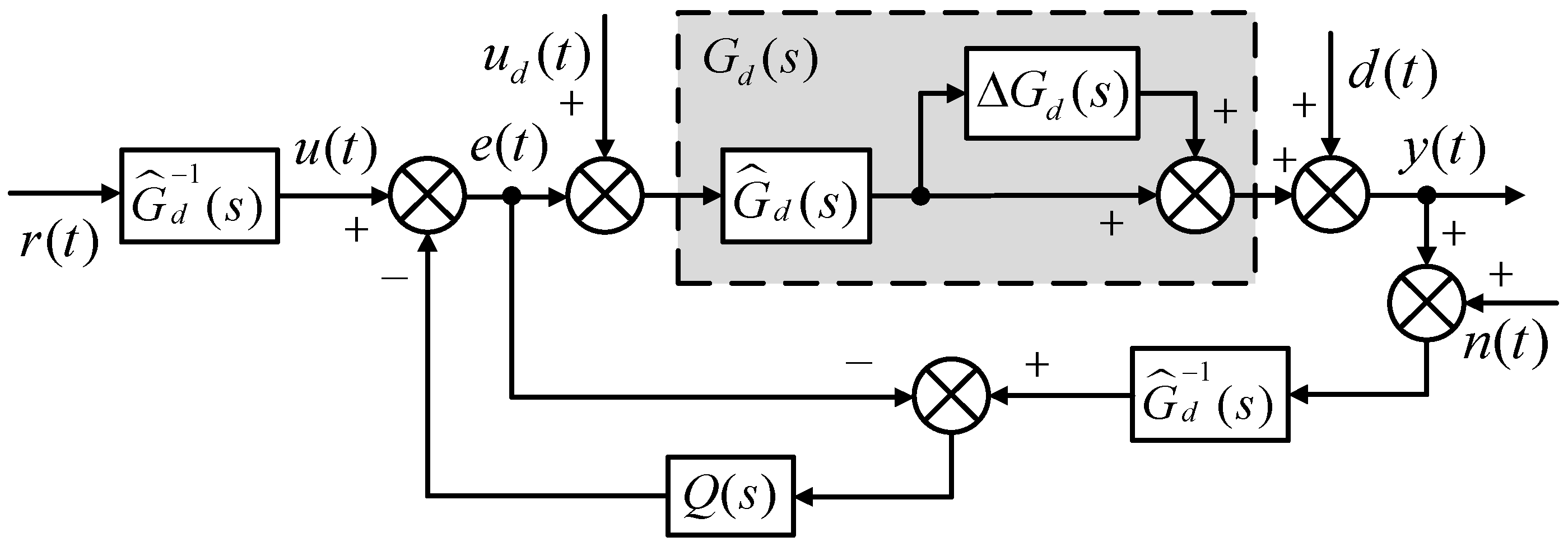
3.4. Observer-Based Inverse Control Compensation Scheme

The disturbance observer as the most effective compensation control method has been widely used in various applications, which have disturbance, parameter uncertainty, noise signals and system nonlinearity, etc., and has a satisfactory control effect [36,48]. Thus, in this paper, the disturbance observer cooperating with the feed-forward inverse controller is adopted to the dual-shaking table control system to restrain the system disturbance to obtain good tracking performance, as is shown in Figure 11.

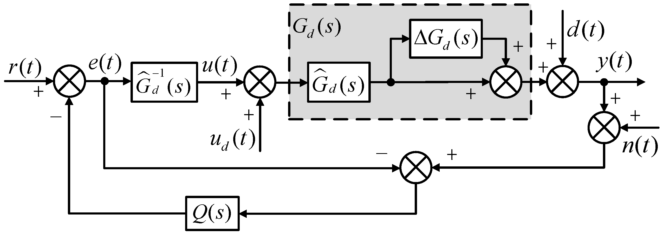
From Figure 11, it can be seen that the disturbance observer needs to use the close-loop control system inverse model. Also, the cross-coupled control action u_d(t) needs to be separated from the total control signal to avoid the effect on tracking precision. Based on the analysis, this paper proposes a novel simple disturbance observer without the system inverse model and the control u_d(t) also does not need to be separated, as is shown in Figure 12. The proposed control scheme has the same control performance with the original control scheme while simplifying the control system and the control effect is derived as follows.

The $Q(s)$ in Figure 11 and Figure 12 is the low-pass filter to ensure stability and to filter high-frequency noise signals for the control system. The design of f_q not only depends on the frequency range of noise signals but also depends on the robust stability of the control system. Generally, the bigger the frequency width f_q, the better the disturbance restraining effect and the worse it is for the system stability. Above all, the design of f_q should make a trade-off between the robust stability, tracking performance and restraining disturbance. It can be designed as [48]

$$Q(s)=\frac{\frac{1}{2\mathsf{\pi }{f}_q}s+1}{\frac{s^3}{{(2\mathsf{\pi }{f}_q)}^3}+\frac{3}{{(2\mathsf{\pi }{f}_q)}^2}{s}^2+\frac{3}{2\mathsf{\pi }{f}_q}s+1}$$

(37)

Combining Equations (32) and (33), the system outputs derived from Figure 11 and from Figure 12 are completely identical and can be written as

$$\begin{array}{ll}{y}^{\prime }(t)& =\frac{\left[1+\Delta {\widehat{G}}_d(s)\right]\left[1+\Delta G_d(s)\right]\left[r(t)-Q(s)n(t)\right]}{1+Q(s)\left[\Delta {\widehat{G}}_d(s)+\Delta G_d(s)+\Delta {\widehat{G}}_d(s)\Delta G_d(s)\right]}\\ & +\frac{\left[1-Q(s)\right]{\widehat{G}}_d(s)\left[1+\Delta G_d(s)\right]u_d(t)+\left[1-Q(s)\right]d(t)}{1+Q(s)\left[\Delta {\widehat{G}}_d(s)+\Delta G_d(s)+\Delta {\widehat{G}}_d(s)\Delta G_d(s)\right]}\end{array}$$

(38)

Combining Equation (38), the control system errors from the two control scheme of Figure 11 and Figure 12 are completely identical and can be described as

$$\begin{array}{ll}{e}^{\prime }(t)& =r(t)-y^{\prime }(t)\\ & =\frac{\left[Q(s)-1\right]\left[\Delta {\widehat{G}}_d(s)+\Delta G_d(s)+\Delta {\widehat{G}}_d(s)\Delta G_d(s)\right]r(t)}{1+Q(s)\left[\Delta {\widehat{G}}_d(s)+\Delta G_d(s)+\Delta {\widehat{G}}_d(s)\Delta G_d(s)\right]}\\ & +\frac{\left[Q(s)-1\right]{\widehat{G}}_d(s)\left[1+\Delta G_d(s)\right]u_d(t)+\left[Q(s)-1\right]d(t)}{1+Q(s)\left[\Delta {\widehat{G}}_d(s)+\Delta G_d(s)+\Delta {\widehat{G}}_d(s)\Delta G_d(s)\right]}\\ & +\frac{Q(s)\left[1+\Delta {\widehat{G}}_d(s)\right]\left[1+\Delta G_d(s)\right]n(t)}{1+Q(s)\left[\Delta {\widehat{G}}_d(s)+\Delta G_d(s)+\Delta {\widehat{G}}_d(s)\Delta G_d(s)\right]}\end{array}$$

(39)

From the derived results Equations (38) and (39), it can be demonstrated that the control scheme in Figure 12 has the same control performance with that in Figure 11. Generally, the system noise signals are always high-frequency signals, so the noise signals filtered by the low-pass filter $Q(s)$ have little effect on the system control precision and can be ignored. Furthermore, $Q(s)$ is the low-pass filter, so in a certain low frequency range, there exists $Q(s)\approx 1$ and combining Equation (39), it can be derived that the control system errors $e^{\prime }(t)\approx 0$, that is to say, the system error caused by identified system model error, designed inverse model error, r(t), u_d(t), d(t) and n(t) can be eliminated through the proposed simple disturbance observer cooperating with the feed-forward inverse controller. In addition, it also can be seen that the compound control strategy causes the identified model and the designed inverse model to have some errors, which can avoid the obtainment of the exact system model and inverse model.

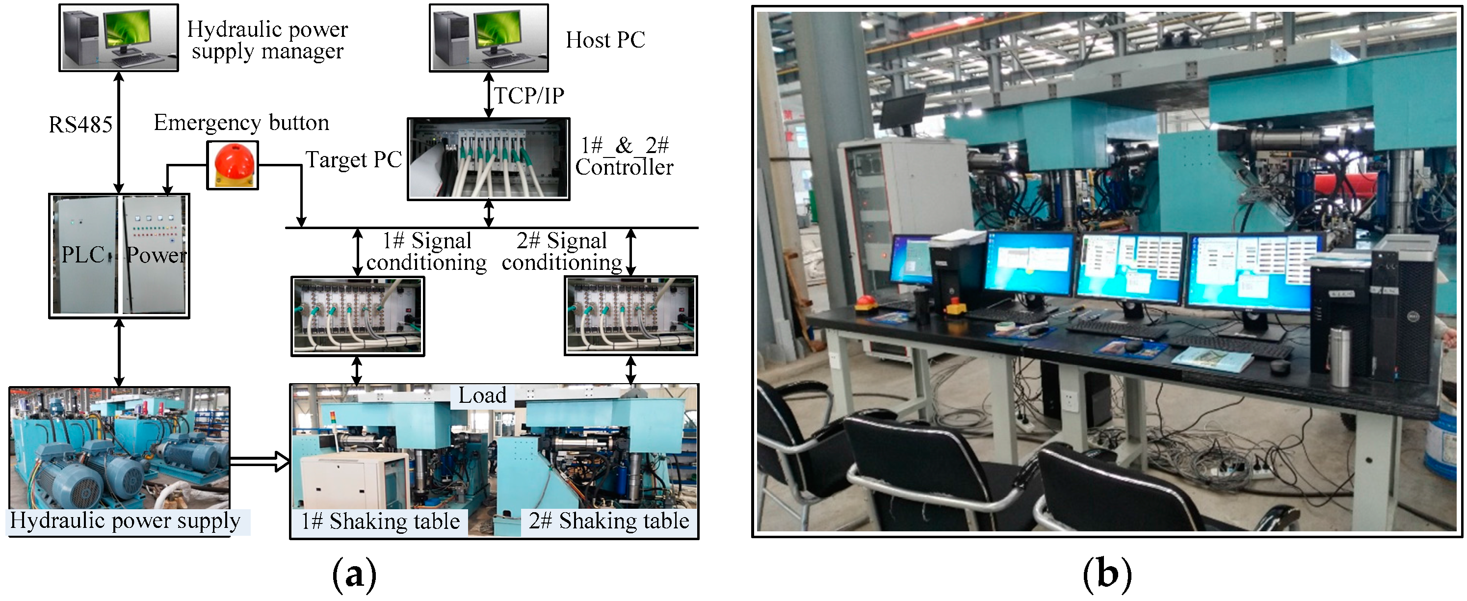
4. Experimental Results

To verify the effectiveness of the proposed control scheme in this paper, the dual-shaking table host-to-target real-time control experiment system shown in Figure 13 is built based on a rapid prototype technique and a variety of experiments are performed. The control system mainly contains several parts: task management unit, hydraulic power supply management unit, hydraulic power supply unit, servo motion control unit, signal conditioning unit, signal acquisition unit, shaking tables and the test specimen. The target PC is the National Instrument computer PXI-1044, including the controller PXI-8119, the A/D cards PXI-6259, D/A cards PXI-6733, digital I/O card PXI-6508. The task management unit monitors and controls the servo motion control unit through the TCP/IP communication protocol, respectively. The proposed control strategy is programmed using the Matlab/Simulink and then complied to target PC for real-time control execution. The control signals from motion control unit will be processed in the signal conditioning unit and then are sent to the servo valves in the form of input current to control the motion of hydraulic cylinders, which in turn drive the dual-shaking table to move with desired trajectory. The sample time of real-time controller is 1 ms.

The experiment tests mainly contain four parts: servo valve tests, IFS and GBC tests, synchronization control tests and tracking control tests. Note that although the shaking table has six DOFs, whose structure is to realize the three translations and reduce the coupling action of the three directions, the experiment tests are generally performed only in three translation directions. It is because the earthquake waveform and anti-earthquake research are both only in the three translation directions, which has been shown in many practical applications [7,49,50]. Thus, the experiment tests in this paper are performed in X/Y/Z translation directions. Note that the TVC mentioned in Section 3 runs in the displacement control and all the experiment tests except for the servo valve tests in this paper are performed with the specimen described in Section 2.1.

The DOF synthesis matrix H_h in Figure 8 is obtained according to a geometrical relationship

$$H_h=\left[\begin{array}{cccccccc}0.5& 0& -0.5& 0& 0& 0& 0& 0\\ 0& 0.5& 0& -0.5& 0& 0& 0& 0\\ 0& 0& 0& 0& 0.25& 0.25& 0.25& 0.25\\ 0& 0& 0& 0& -0.018& -0.018& 0.018& 0.018\\ 0& 0& 0& 0& -0.018& 0.018& 0.018& -0.018\\ -0.11& -0.11& 0.11& 0.11& 0& 0& 0& 0\end{array}\right]$$

(40)

The DOF decomposition matrix H_f in Figure 8 is the pseudo-inverse of H_h

$$H_f=pinv(H_h)=\left[\begin{array}{cccccc}1& 0& 0& 0& 0& -22.32\\ 0& 1& 0& 0& 0& -22.32\\ -1& 0& 0& 0& 0& 22.32\\ 0& -1& 0& 0& 0& 22.32\\ 0& 0& 1& -13.5& -13.5& 0\\ 0& 0& 1& -13.5& 13.5& 0\\ 0& 0& 1& 13.5& 13.5& 0\\ 0& 0& 1& 13.5& -13.5& 0\end{array}\right]$$

(41)

The inner force matrix is derived as [20]

$$H_{if}=I-H_h^T{H}_f^T=\left[\begin{array}{cccccccc}0.25& 0.25& 0.25& 0.25& 0& 0& 0& 0\\ 0.25& 0.25& 0.25& 0.25& 0& 0& 0& 0\\ 0.25& 0.25& 0.25& 0.25& 0& 0& 0& 0\\ 0.25& 0.25& 0.25& 0.25& 0& 0& 0& 0\\ 0& 0& 0& 0& 0.25& 0.25& -0.25& -0.25\\ 0& 0& 0& 0& 0.25& 0.25& -0.25& -0.25\\ 0& 0& 0& 0& -0.25& -0.25& 0.25& 0.25\\ 0& 0& 0& 0& -0.25& -0.25& 0.25& 0.25\end{array}\right]$$

(42)

4.1. Servo Valve Tests

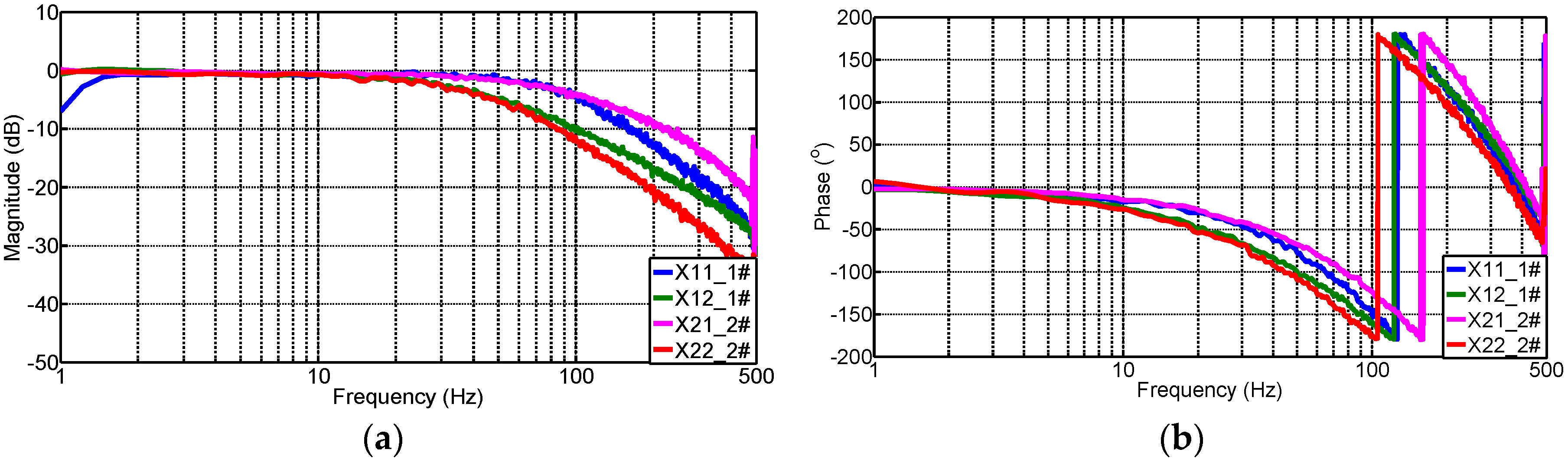
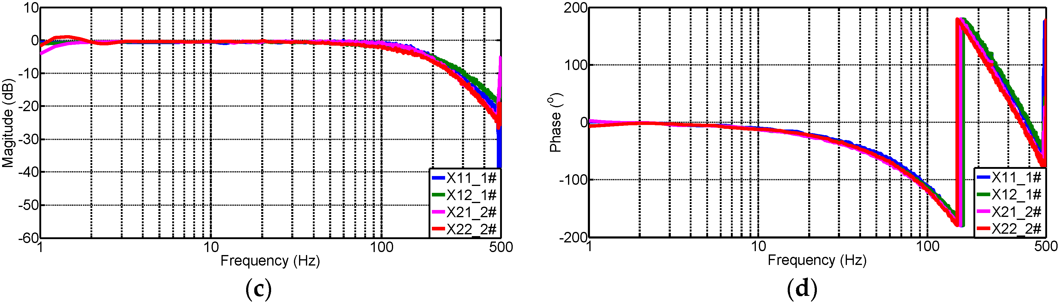
The servo valve experiment tests are performed to test performances of the developed servo valves. As is mentioned in Section 2.3, in order to obtain better consistency and performance of valves, the valve controller as the electric part of the valve is designed to realize the displacement close-loop control of the three-stage servo valve shown in Figure 3c and has several tunable parameters: the offset of pilot valve and main valve spool, displacement feedback gain, velocity feedback gain and feed-forward gain. During the tuning of valve tunable parameters, first the offsets of the pilot valve and main valve spool are tuned to reduce the offset of valves’ output displacements under the static constant input signals; then, the displacement feedback gain and velocity feedback gain are tuned to obtain a better dynamic response performance under step input signals; at last, the feed-forward gain is tuned to further improve the dynamic performance of the servo valve. The step signal is given to servo valves simultaneously and the step response signals of the servo valves are compared. The parameters of valve controllers are tuned until the servo valves have approximately similar step response times and overshoots under the same step signal. For the frequency characteristic, 10% of full span random signals are given to servo valves before and after tuning the parameters of valve controllers, respectively. The magnitude frequency characteristics and phase frequency characteristics estimated are shown in Figure 14.

From Figure 14, it can be seen that before tuning valve controllers, the performances of servo valves are different from each other and the minimum magnitude frequency width is less than 60 Hz, which can influence the control system precision significantly. After tuning valve controllers, the performances are approximately the same and the magnitude frequency width is more than 100 Hz, which indicates that the developed servo valves with parameter-tunable valve controllers can improve the servo valves' performances significantly. The experiment results for all servo valves in three directions are similar, so in Figure 14 only the four servo valves in X direction are listed for simplicity.

4.2. IFS and GBC Tests

This part will test the IFS and GBC. To make the verification adequate, various experimental tests are performed using different control strategies. The experimental results are approximately identical for the two shaking tables, so only the results of the first one are listed in the figures and tables for simplicity.

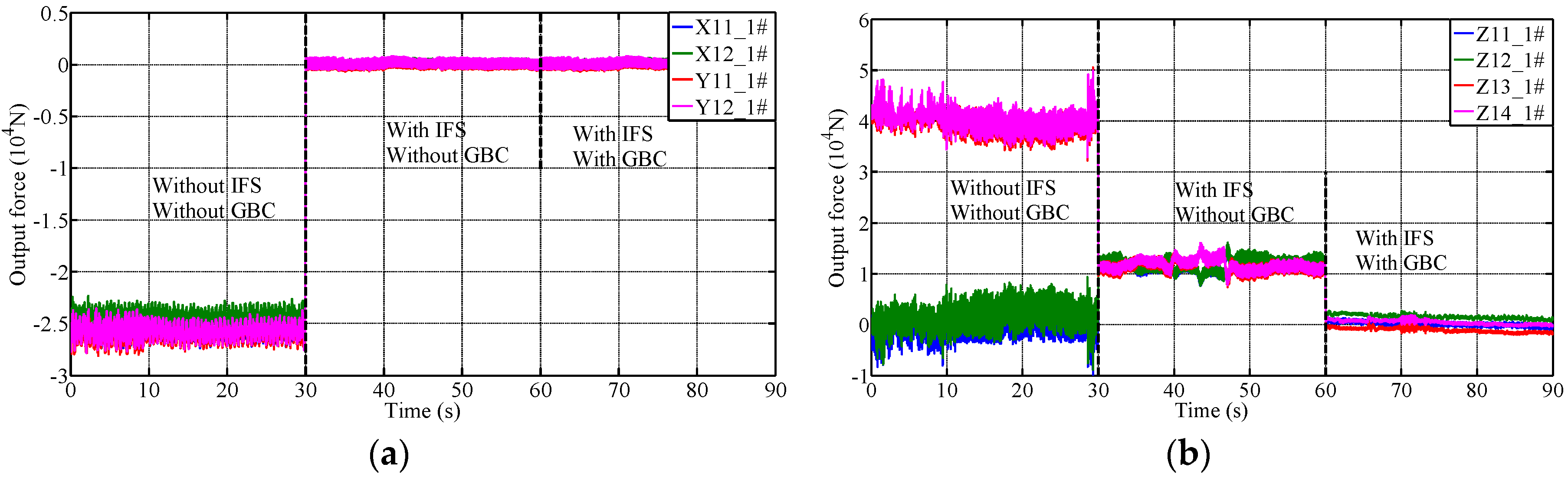
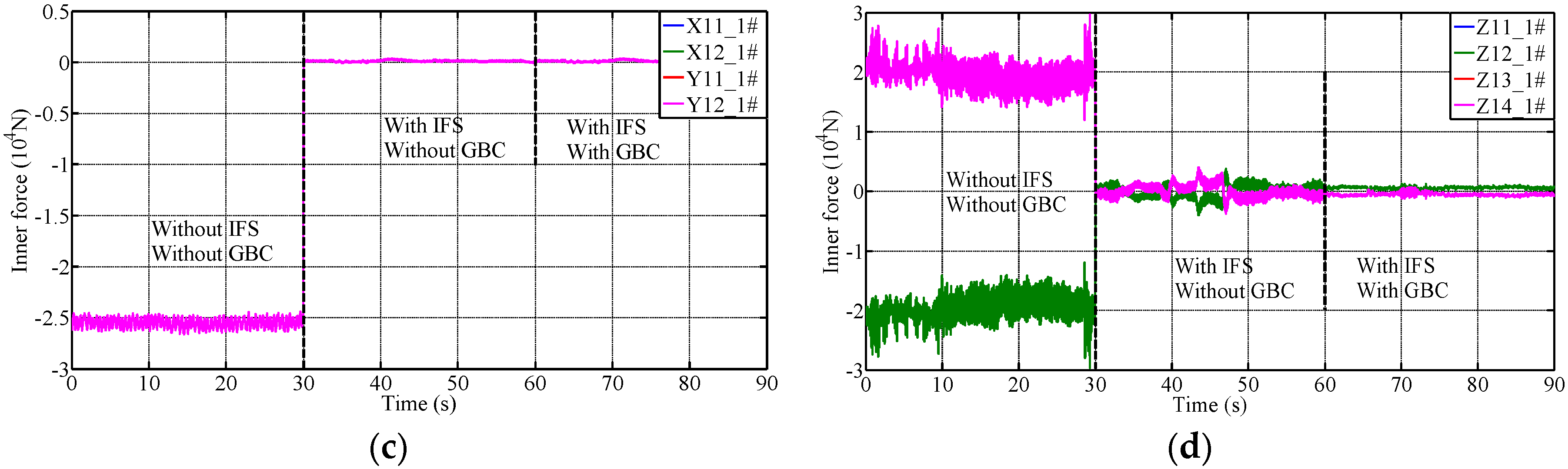
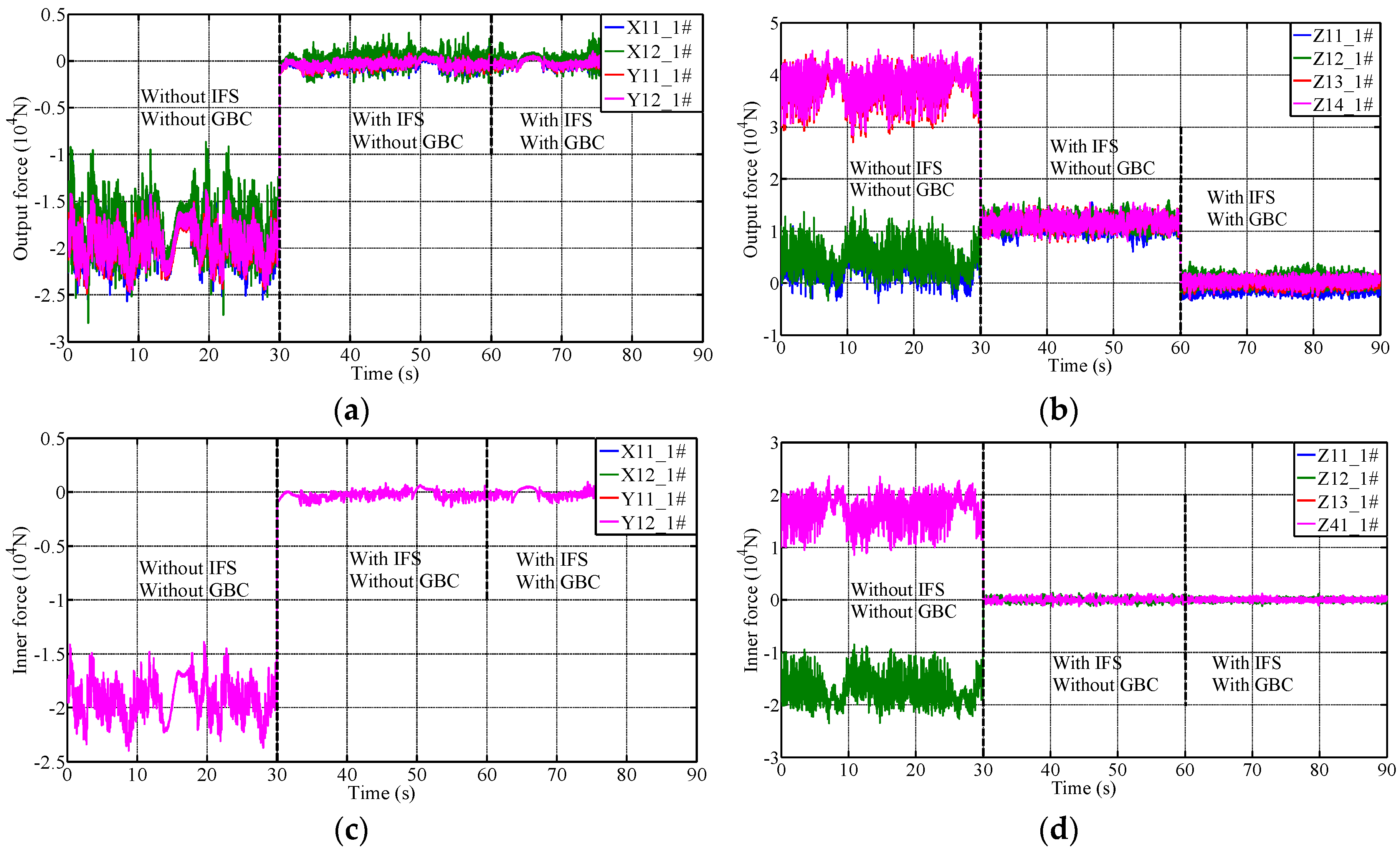
For different control strategies, Figure 15 and Figure 16 show the output forces and inner forces of hydraulic cylinders when the shaking table is static at the 0 position and under the random signal excitation, respectively. Each figure is divided into three phases: the first phase is without IFS and without GBC, the second phase is with IFS and without GBC and the third phase is with both IFS and GBC, and each phase lasts 30 s. The detailed data comparisons of inner forces and output forces are tabulated in

Table 2. The maximum inner forces and output forces with different controllers at 0 position.

Output Forces/Inner Forces	Without Inner Force Suppression (IFS), Gravity Balance Control (GBC)	With IFS, without GBC	With IFS, GBC
Horizontal output forces	2.8 × 104 N	500 N	500 N
Horizontal inner forces	2.6 × 104 N	200 N	200 N
Vertical output forces	4.8 × 104 N	1.4 × 104 N	1200 N
Vertical inner forces	2.7 × 104 N	2000 N	1000 N

and

Table 3. The maximum inner forces and output forces with different controllers under random signals.

Output Forces/Inner Forces	Without IFS, GBC	With IFS, without GBC	With IFS, GBC
Horizontal output forces	2.5 × 104 N	3000 N	3000 N
Horizontal inner forces	2.3 × 104 N	600 N	600 N
Vertical output forces	4.4 × 104 N	1.4 × 104 N	3000 N
Vertical inner forces	2.2 × 104 N	1000 N	1000 N

, which counts the maximum values. Note that the output forces in the figures and tables are used to demonstrate the validity of the designed GBC, which is used to reduce the output forces of vertical hydraulic cylinders by balancing the gravity of table and load. The inner forces of hydraulic cylinders are the partial output forces not making any real contribution to the shaking table’s motion. Also, the inner forces are obtained according to the output forces and inner force matrix Equation (42). The inner forces of hydraulic cylinders in the figures and tables are used to demonstrate the validity of the adopted IFS.

From Figure 15 and Figure 16 and Table 2 and Table 3, it can be seen that without IFS and GBC the inner forces and output forces of the hydraulic cylinders are both very large (2.2 × 10⁴–2.7 × 10⁴ N, 2.5 × 10⁴–4.8 × 10⁴ N) due to the inevitable offset of the servo valves, electronic system and mechanical assembly, etc. After using the IFS, the output forces and inner forces of hydraulic cylinders are reduced significantly (200–2000 N, 500–1.4 × 10⁴ N), which indicates that the adopted IFS control strategy can reduce the output forces and inner forces effectively under the same condition and thus reduce the energy consumption and the forces acting on the table. However, the output forces of vertical hydraulic cylinders are still relatively large because of the gravity of the table and load. After using the GBC, the forces are reduced from 1.4 × 10⁴ N to about 1200 N, which indicates that the GBC can balance the gravity of the table and load and reduce the output forces of the vertical hydraulic cylinders. From the above, it can be concluded that the IFS and GBC control strategies are feasible and effective.

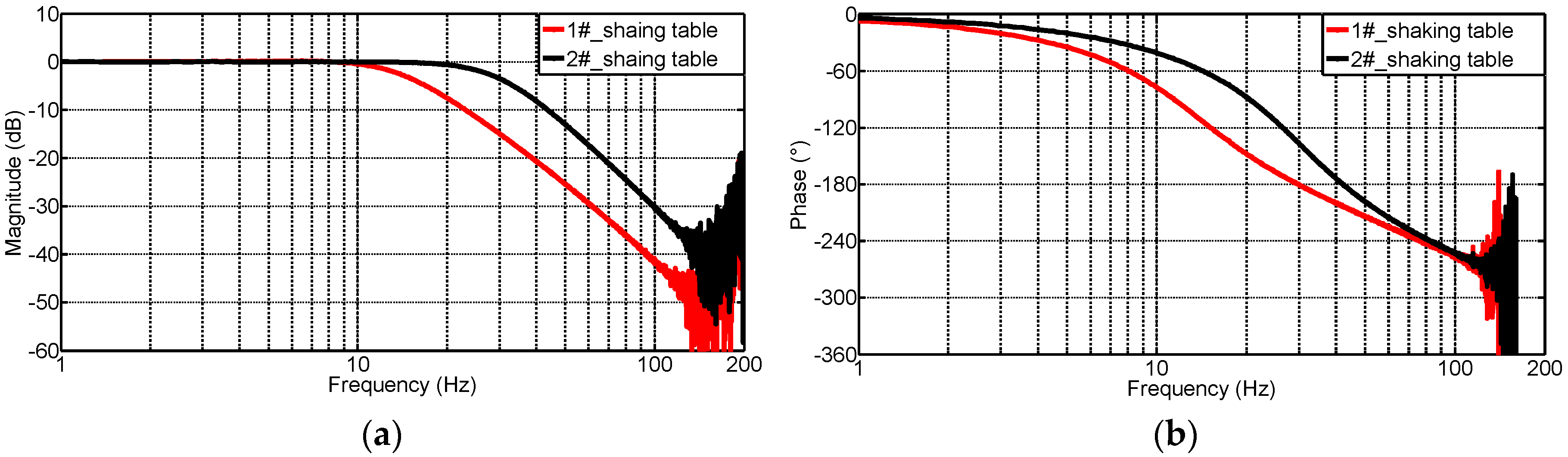
4.3. Synchronization Control Experiment Tests

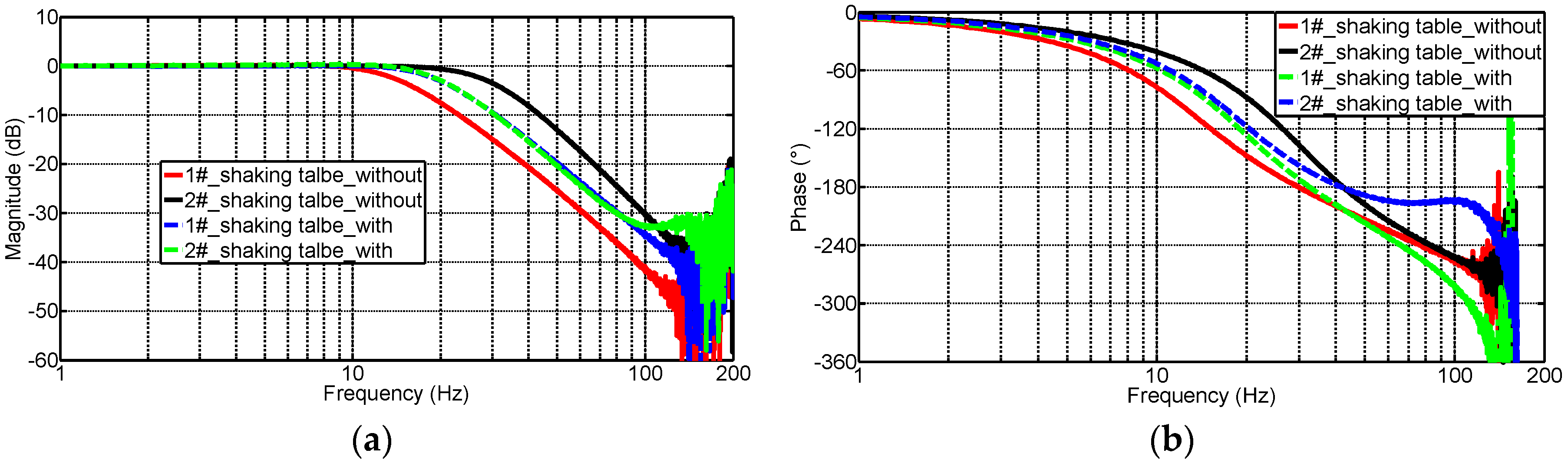
The system frequency response performances before using the synchronization control are tested under random excitation with a peak-peak value of ±1 mm and a frequency range of 0.1–100 Hz. The system frequency response characteristics of the dual-shaking table system are shown in Figure 17. It can be seen that there is large difference between the two shaking tables both in magnitude and phase frequency characteristics, which can cause the large synchronization error when the shaking tables move. Note that the experimental results demonstrate that the control effect of the proposed control scheme are similar in all DOFs, so this part and the next part will list only the ZDOF experimental results for simplicity.

The step signal or random signal is given to tune the parameters of the proposed ASMC and traditional SMC, through watching the synchronization error of the two shaking tables. First, set all these parameters to 0 and then increase the parameters' values to reduce the synchronization error until the error stops reducing. The final tuned parameters are shown in

Table 4. The parameters of the sliding mode control based on adaptive reaching law (ASMC) and traditional sliding mode control (SMC).

Controller	${\mathit{k}}_{\mathit{s}}$	${\mathsf{\beta }}_{\mathit{s}}$	$\mathit{c}$	$\mathsf{\gamma }$
Traditional SMC	6.4	0.95	0	0
ASMC	8.6	1.2	4	0.6

corresponding to the following experimental results.

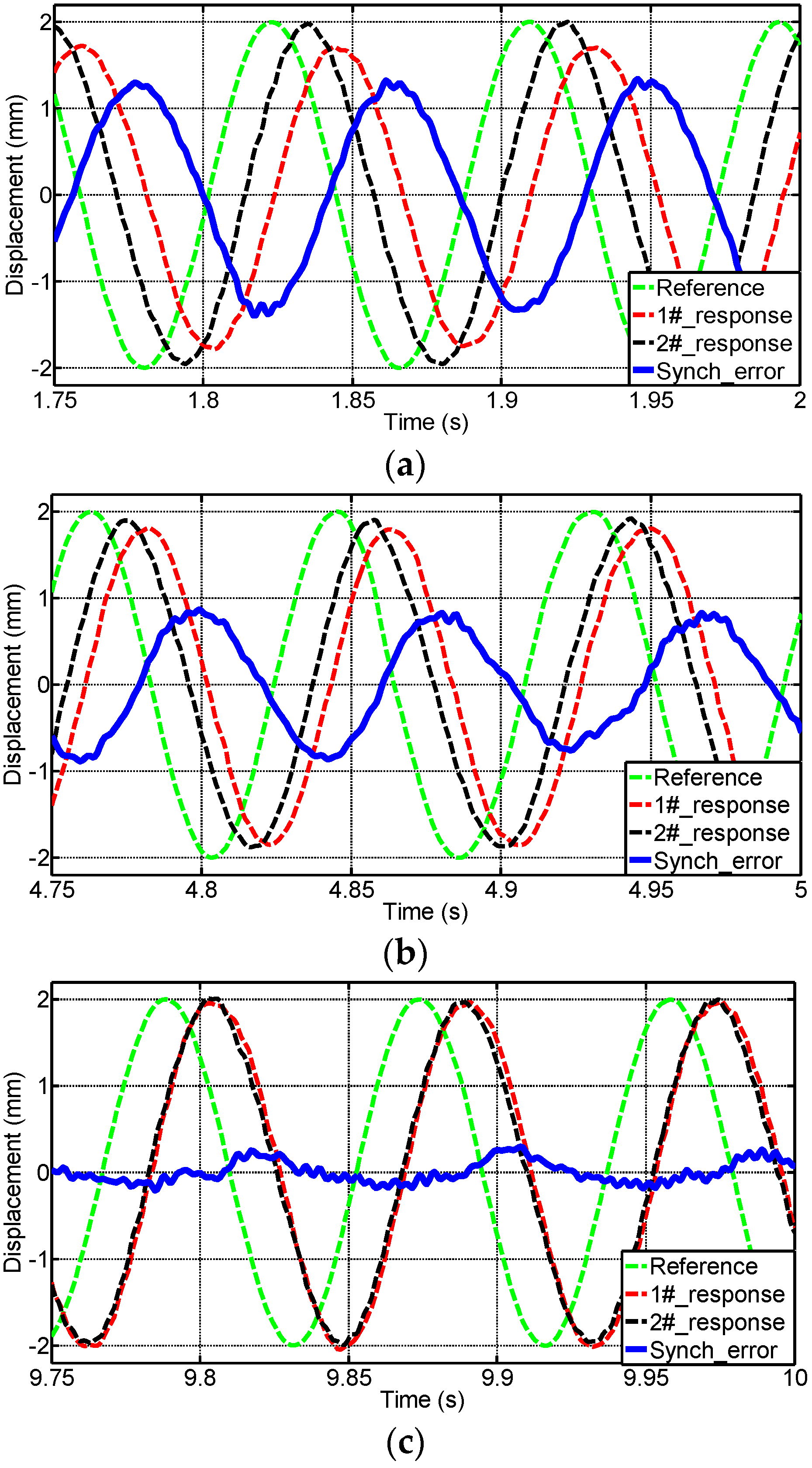
For the purpose of comparison, the synchronization control experiments are performed under sine signal and random signal excitations using the proposed ASMC controller and traditional SMC controller, respectively. The 2 mm 12 Hz sine signal experiment results are shown in Figure 18, from which it can be seen that the maximum synchronization error is 1.301 mm without synchronization control and the error is reduced to 0.866 mm and 0.3 mm using the traditional SMC and proposed ASMC synchronization controller, respectively.

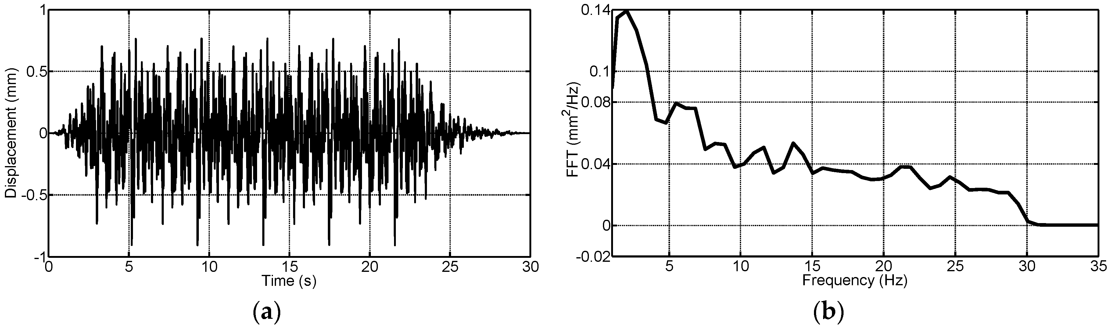
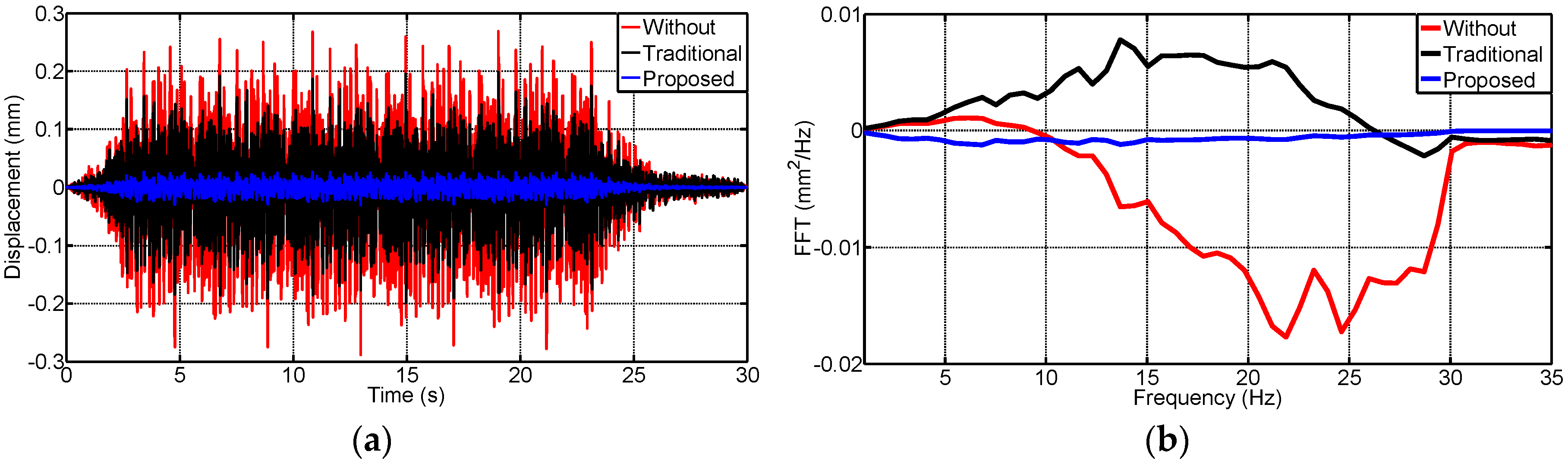
The random signal excitations with amplitude of ±1 mm and frequency range of 0.1 Hz–30 Hz are used to test different controllers. The reference signal in the time domain and frequency domain are shown in Figure 19. Also, the experimental results of the synchronization errors are shown in Figure 20. The detailed data comparisons of errors are tabulated in

Table 5. Synchronization errors under random signal.

Controller	Without	Traditional	Proposed
Maximum errors	0.2888 mm	0.1994 mm	0.0306 mm
Root mean square (RMS) errors	0.0854 mm	0.056 mm	0.0089 mm

, which counts the maximum errors and root mean square (RMS) errors.

From Figure 20 and Table 5, the maximum and RMS of synchronization errors are from 0.2888 mm to 0.0306 mm and from 0.0854 mm to 0.0089 mm, which is almost reduces to 10% and demonstrates that the proposed synchronization controller is feasible and efficient. Figure 21 shows the system frequency response characteristics with the proposed ASMC synchronization controller, which demonstrates that the two shaking tables with the proposed synchronization controller have similar frequency characteristics.

4.4. Tracking Control Experiment Tests

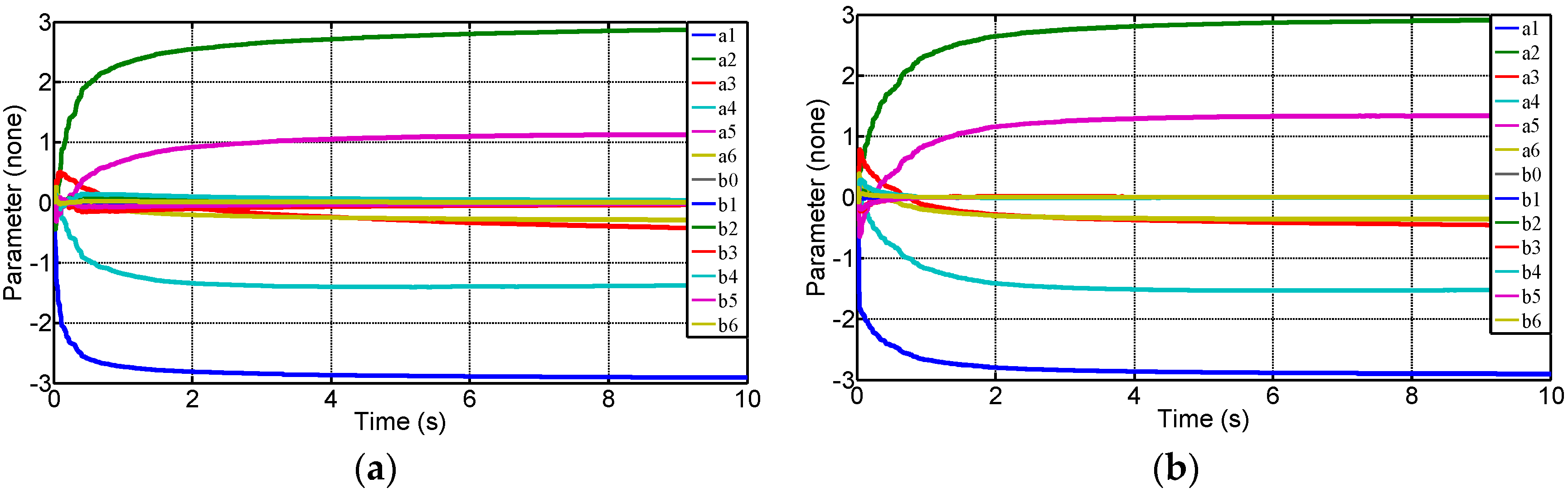
The random signal excitations with an amplitude of ±1 mm and frequency range of 0.1 Hz–100 Hz are performed to identify the system transfer function according to the reference signal and response signal using the RLS algorithm. The system model parameters are shown in Figure 22 and the identified discrete transfer functions are expressed as

$$\begin{array}{l}{\widehat{G}}_d(z)=\frac{1.3052\times {10}^{-3}(z^2-0.8966z+0.3641)(z^2-1.126z+1.366)(z^2-3.972z+7.417)}{(z+0.7426)(z-0.7161)(z^2-1.856z+0.8684)(z^2-1.076z+0.6268)}\\ {\widehat{G}}_{d2}(z)=\frac{1.8497\times {10}^{-4}(z-10.9)(z+0.5198)(z^2-1.265z+0.5542)(z^2+1.681z+1.98)}{(z+0.7768)(z-0.7411)(z^2-1.859z+0.8713)(z^2-1.079z+0.725)}\end{array}$$

(43)

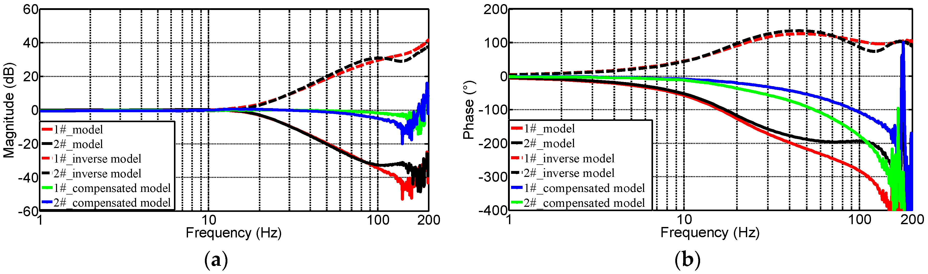
The feed-forward inverse transfer function according to Equation (31) can be obtained as

$$\begin{array}{ll}{\widehat{G}}_d^{-1}(z)& =\frac{(z+0.7426)(z-0.7161)(z^2-1.856z+0.8684)(z^2-1.076z+0.6268)}{1.3052\times {10}^{-3}(z^2-0.8966z+0.3641)}\\ & \times \frac{(z^{-2}-1.126z^{-1}+1.366)(z^{-2}-3.972z^{-1}+7.417)}{{(1-1.126+1.366)}^2{(1-3.972+7.417)}^2{z}^4}\\ {\widehat{G}}_{d2}^{-1}(z)& =\frac{(z+0.7768)(z-0.7411)(z^2-1.859z+0.8713)(z^2-1.079z+0.725)}{1.8497\times {10}^{-4}(z+0.5198)(z^2-1.265z+0.5542)}\\ & \times \frac{(z^{-1}-10.9)(z^{-2}+1.681z^{-1}+1.98)}{{(1-10.9)}^2{(1+1.681+1.98)}^2{z}^3}\end{array}$$

(44)

From Equations (43) and (44), the frequency characteristics of the identified system models and the designed inverse models are shown in Figure 23.

Note that the G_d and G_d2 in Equation (43) seem to be noticeably different even though the tables are supposed to be synchronized. The noticeable difference in Equation (43) is mainly due to the fact that the order of the identified model is relatively high and there is some difference when the frequency is relatively high, as shown in Figure 23. Especially, the difference of the phase characteristic of the two tables is noticeable. However, the G_d and G_d2 have the similar characteristics when the frequency is not too high both in magnitude and phase characteristics, as shown in Figure 23 and we are concerned within the characteristics within the medium and low frequency range. So, the obtained results for G_d and G_d2 in Equation (43) are correct and reasonable.

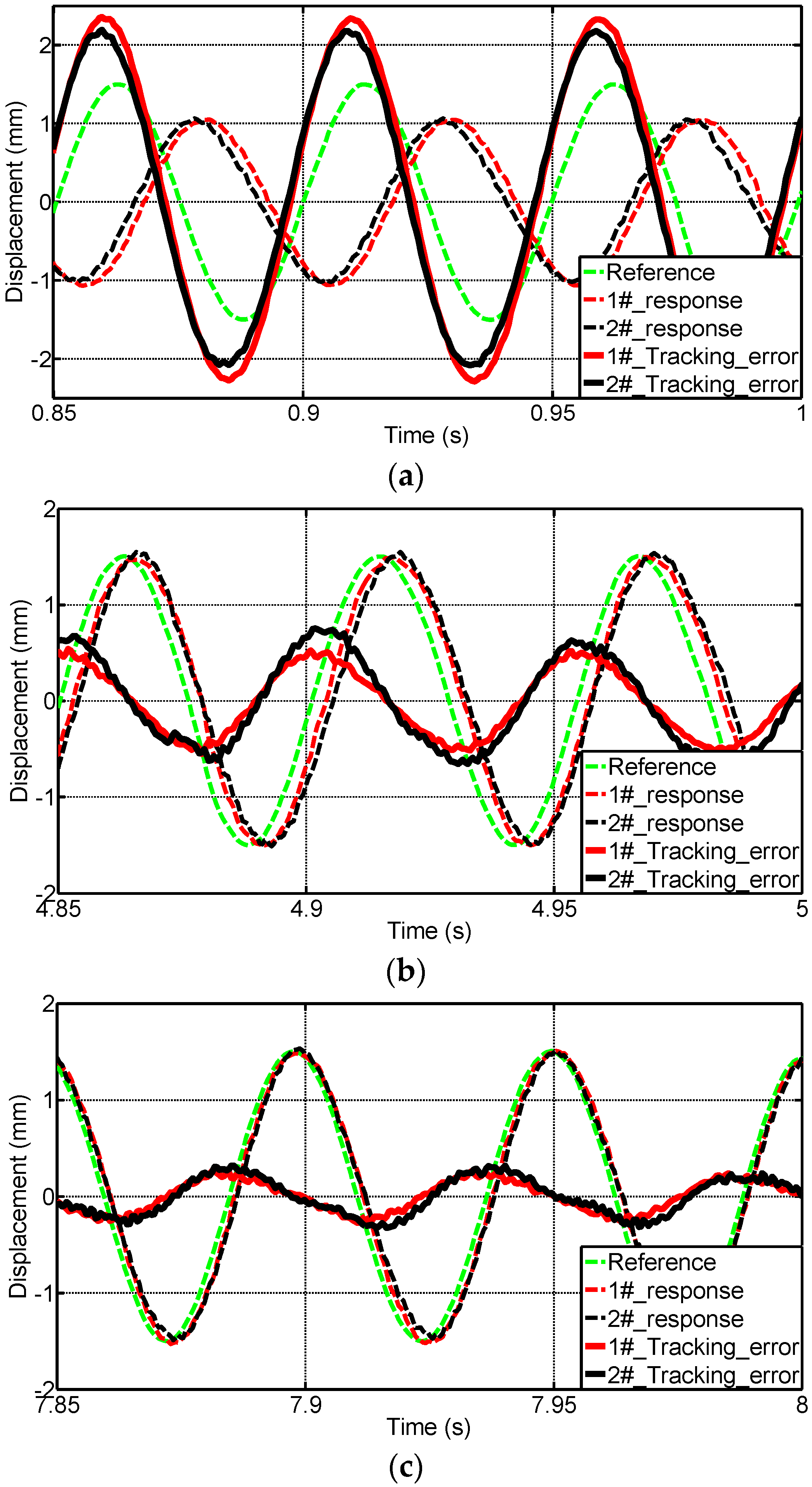
To verify the proposed tracking controller shown in Figure 12, the 1.5 mm 20 Hz sine signals are given and the test results are shown in Figure 24. Note that the tracking control tests below are both with the proposed ASMC synchronization controller. Also, the frequency parameter f_q in Equation (37) is 48 Hz during the experimental tests. It can be seen in Figure 24a that the maximum tracking errors are 2.328 mm/2.18 mm using the traditional controller, which is even larger than the maximum of the given signal due to the large phase lag of the system. The errors reduce to 0.7435 mm/0.5042 mm with the feed-forward inverse model controller and reduce to 0.3169 mm/0.2109 mm with the proposed tracking controller, which is almost 13%/9% of that of the traditional controller.

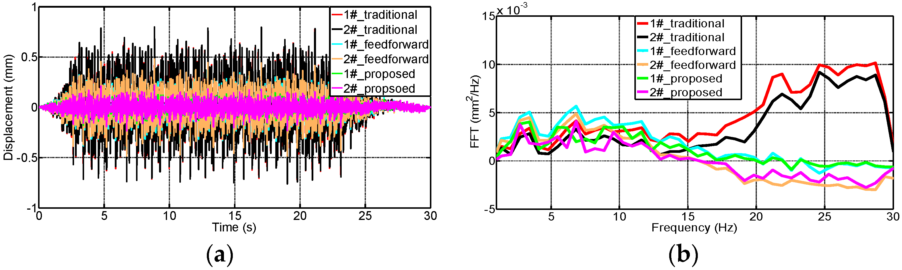
The random signal tests are performed to further verify the proposed tracking controller. The random signal used in this section is the same as in Section 4.3, shown in Figure 19. The tracking errors both in the time domain and frequency domain of the two shaking tables using different controllers are shown in Figure 25. The detailed data comparisons of tracking errors are tabulated in

Table 6. Tracking errors under random signal.

Maximum/RMS Errors	Traditional	Feedforward	Proposed
Maximum errors	0.735 mm/0.8015 mm	0.4405 mm/0.4848 mm	0.181 mm/0.2331 mm
RMS errors	0.2425 mm/0.2514 mm	0.1173 mm/0.1227 mm	0.0454 mm/0.05 mm

, which counts the maximum errors and RMS errors. From Figure 25 and Table 6, it can be obtained that the maximum tracking errors using the traditional controller are 0.735 mm/0.801 mm, which is close to the maximum reference signal. The errors are reduced to 0.181 mm/0.233 mm with the proposed controller. Also, we can see from Figure 25b that the tracking errors decrease at the full frequency range with the proposed controller compared with traditional and feed-forward controllers.

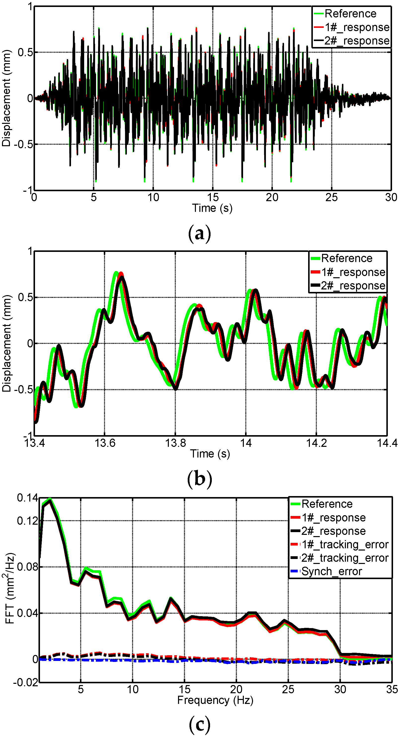
Figure 26 shows the experimental results in the time domain and frequency domain with the proposed compound control scheme combining the proposed ASMC synchronization controller and observer-based feed-forward inverse compensation tracking controller, from which it can be seen that the proposed compound control scheme can cause the two shaking tables to move with high tracking precision and synchronization precision. 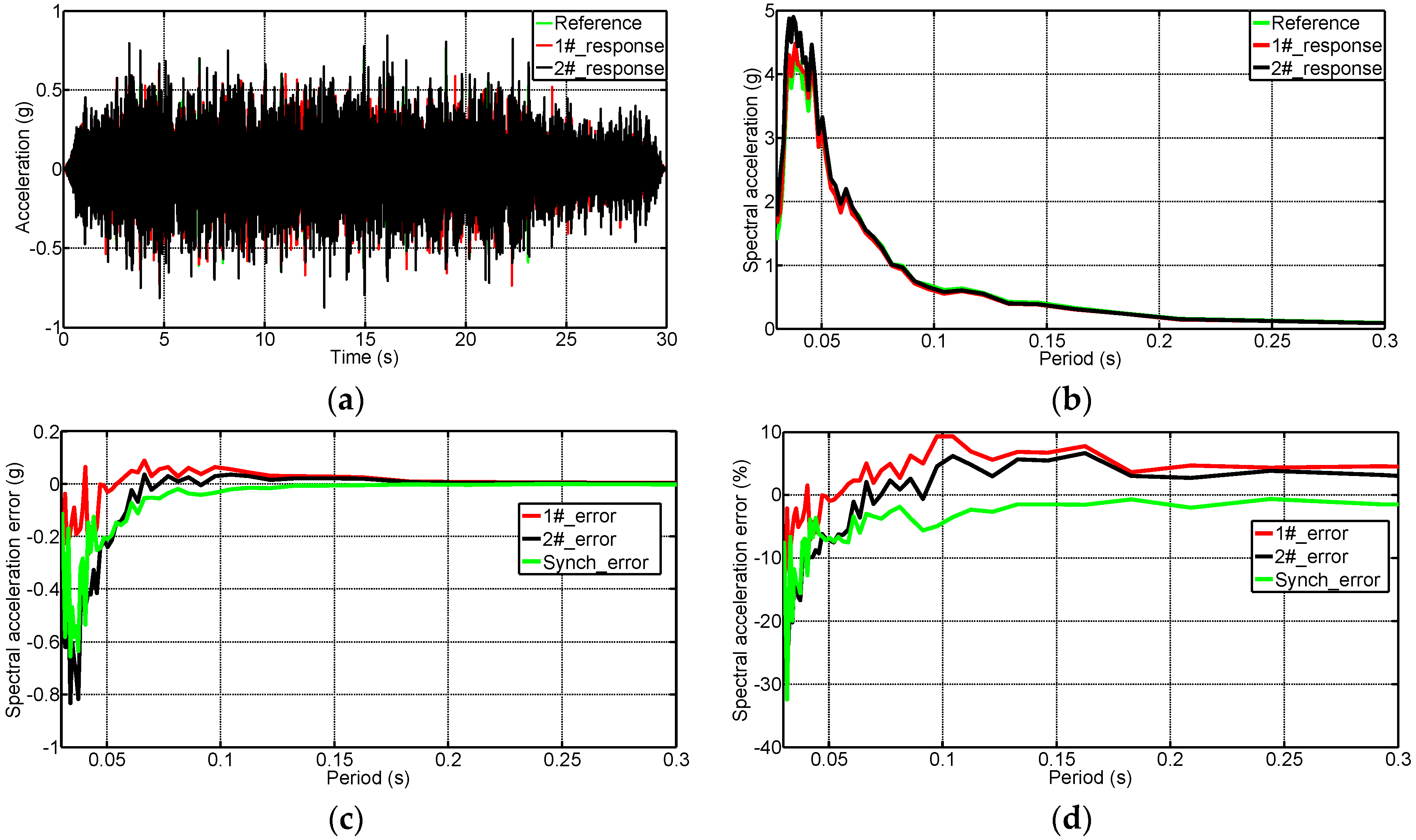Figure 27 shows the response spectral acceleration of the reference and achieved accelerations in the [0.03, 0.3] s natural period band for 2% damping under the proposed compound control scheme.

5. Conclusions

In this paper, an electro-hydraulic dual-shaking table system is developed and the system parameters are designed and optimized in detail. To improve the attitude synchronization and tracking control precision, a novel hybrid control scheme is proposed, which is a combination of the novel ASMC cross-coupled controller and the observer-based feed-forward inverse compensation controller. The ASMC is introduced to the cross-coupled controller to reduce synchronization error, and the observer-based feed-forward inverse controller is proposed to improve tracking precision.

The dual-shaking table experiment system is built based on the xPC target technique and various comparison experiments are performed. The servo valve experimental results indicate that the developed servo valve with a parameter-tunable valve controller can improve the consistency and extend the servo valve frequency width from 60 Hz to 100 Hz. The IFS and GBC experimental results show that the control strategy can reduce the hydraulic cylinders’ maximum inner forces from 2.7 × 10⁴ N to 2000 N and maximum output forces from 4.8 × 10⁴ N to 1200 N, respectively. The synchronization and tracking experimental results demonstrate that the proposed ASMC can reduce the RMS synchronization error from 0.056 mm to 0.0089 mm, which is almost 15.8% lower compared with the traditional controller. The proposed tracking controller can reduce the RMS tracking errors from 0.735 mm/0.801 mm to 0.181 mm/0.233 mm, which is about 24.6%/29% of the former. Experimental results demonstrate that the developed dual-shaking tables system with the proposed hybrid control scheme can allow synchronization and tracking control of a dual-shaking table with high precision.