Rail-STrans: A Rail Surface Defect Segmentation Method Based on Improved Swin Transformer

Abstract

With the continuous expansion of the transport network, the safe operation of high-speed railway rails has become a crucial issue. Defect detection on the surface of rails is a key part of ensuring the safe operation of trains. Despite the progress of deep learning techniques in defect detection on the rails’ surface, there are still challenges related to various problems, such as small datasets and the varying scales of defects. Based on this, this paper proposes an improved encoder–decoder architecture based on Swin Transformer network, named Rail-STrans, which is specifically designed for intelligent segmentation of high-speed rail surface defects. The problem of a small and black-and-white rail dataset is solved using self-made large and multiple rail surface defect datasets through field shooting, data labelling, and data expansion. In this paper, two Local Perception Modules (LPMs) are added to the encoding network, which helps to obtain local context information and improve the accuracy of detection. Then, the Multiscale Feature Fusion Module (MFFM) is added to the decoding network, which helps to effectively fuse the feature information of defects at different scales in the decoding process and improves the accuracy of defect detection at multiple scales. Meanwhile, the Spatial Detail Extraction Module (SDEM) is added to the decoding network, which helps to retain the spatial detail information in the decoding process and further improves the detection accuracy of small-scale defects. The experimental results show that the mean accuracy of the semantic segmentation of the method proposed in this paper can reach 90.1%, the mean dice coefficient can reach 89.5%, and the segmentation speed can reach 37.83 FPS, which is higher than other networks’ segmentation accuracy. And, at the same time, it can achieve higher efficiency.

1. Introduction

The operation environment of high-speed railway lines is becoming increasingly complex due to their continuous expansion. To ensure safe and smooth operation, it is necessary to accurately and rapidly detect defects in rails and other vulnerable parts in complex scenes. This is a prerequisite for achieving high-quality development of high-speed rail. Practice has shown that high-speed rail capacity increases lead to long-term repeated loading, which subjects the rail to contact stresses, such as extrusion, impact, and abrasion, caused by the wheel and rail. Additionally, the microstructure of the material degrades over time, resulting in a continuous deterioration of its health condition and performance quality, leading to the formation of defects. If a defect forms, it can quickly expand. Without timely detection and safety measures, the defect can reach a critical level and cause major accidents, such as train derailments and overturns, resulting in significant casualties and property damage [1].

Manual inspection is a traditional method for detecting defects on rail surfaces. It has the advantages of being simple and cost-effective. However, it also has some shortcomings, including low detection efficiency, high leakage rates, and poor real-time performance [2]. The development of inspection technology has led to the widespread use of non-destructive testing techniques in the railroad inspection system. Commonly used techniques include three-dimensional detection, eddy current detection, and acoustic wave detection [3]. Xiong et al. [4] proposed a three-dimensional laser profiling system (3D-LPS) that integrates multiple sensors to automatically detect and classify rail surface defects. The system significantly improves detection accuracy through high-precision alignment and localization techniques. Cao et al. [5] proposed a scheme for detecting defects on rail surfaces. The scheme uses a laser sensor to collect three-dimensional point cloud data and combines it with an alignment method for digital rail surfaces and improved dynamic defect detection algorithms. This approach effectively eliminates noise and enhances the stability and anti-interference of the detection results. The scheme is suitable for online inspection applications. Liu et al. [6] proposed an online rail defect detection method based on electromagnetic tomography (EMT) technology to obtain the shape and location information of defects by measuring and reconstructing the alternating magnetic signals of rail defects, with the aim of improving inspection efficiency and reducing the risk of accidents caused by rail defects. Fan et al. [7] proposed for the first time a high-precision distributed online rail defect detection method based on backscattered enhanced fiber-optic sensing, which achieves precise positioning of long-distance rail defects through a dual-frequency joint processing algorithm, and the field test shows that the standard deviation is as low as 0.314 m, providing a new technological breakthrough for detecting structural defects in railways and other infrastructure. Kundu et al. [8] investigated the optimum location for placing individual acoustic emission sensors on rails to detect defects, and analyzed the signals to determine group velocities using wavelet transforms to accurately detect defects. However, these methods have the disadvantages of being easily disturbed by various external environments, resulting in difficult signal processing and blind spot detection and poor real-time performance. In recent years, machine vision technology has been widely used in rail surface defect detection due to its advantages of high detection accuracy, high speed, and non-contact. Machine-vision-based rail surface defect detection methods can be divided into traditional machine-learning-based detection methods and deep-learning-based detection methods.

In routine applications of machine vision techniques, experts usually manually analyze the defect images on the rail surface to design features or predefined features. Based on these features, they develop feature-learning algorithms for classification. Li et al. [9] proposed a local normalization algorithm designed to enhance the contrast of rail defect images to facilitate feature extraction. Researchers, such as Dubey [10] and Yuan [11], manually extracted features by analyzing the edges of rail surface defects for defect detection. In addition, He et al. [12] used the inverse P–M (Perona–Malik) diffusion algorithm to detect defects on the rail surface and highlighted the defects by differentially processing the original image with the diffusion image. Although all of these methods are effective for rail surface defect detection, they generally suffer from low accuracy and recall, especially in the detection of linear defects, cracks, and microcracks. Later, Shi et al. [13] used an improved Sobel algorithm to find the available features, which can achieve accurate and efficient localization and extract more precise defect features and parameters while reducing the noise. He et al. [14] also proposed a detection algorithm based on background differencing, which consists of four steps—rail region extraction, background modeling and differencing, threshold segmentation, and image filtering—to improve the detection accuracy. On the other hand, Liu et al. [15] proposed a sorting method combining a gray balance model, phase spectrum, and Otsu threshold segmentation to detect rail defects. Wang et al. [16] proposed a method incorporating a principal component analysis model to identify rail surface defects with color features. These methods improve the detection accuracy to some extent, but the main problem is the lack of generativity. Due to the influence of unfavorable factors, such as changing lighting conditions and deteriorating visual environments, the traditional manual feature machine vision technique is not the best choice.

Artificial intelligence has developed rapidly in recent years, and a lot of neural network structure models with high detection accuracy and speed have appeared, so-deep learning-based detection methods have been mentioned. Combining these models for rail surface defect detection can reduce a lot of human and material resources, with a high degree of detection automation, and improve the accuracy and efficiency of detection results. Kaewunruen et al. [17] apply machine learning techniques for non-destructive detection of track features by analyzing field data at an advanced level to reduce the time and cost of rail inspections, and they demonstrate the potential of certain models, such as linear regression, K-nearest neighbor, gradient boosting, and convolutional neural networks, to improve detection accuracy. Sresakoolchai et al. [18] developed a method to detect defects in rail components through supervised and unsupervised machine learning techniques using rail geometry car data, where deep neural networks and convolutional neural networks showed high accuracy, while applying clustering and association rule analysis to provide insights that can help in rail maintenance. Zhang et al. [19] developed a convolutional neural network method that uses pre-convolution and residual structure to enhance the accuracy of rail damage identification. The method analyzes vibration signals collected by piezoelectric ceramic pads and employs deep learning techniques. Li et al. [20] investigated the application of the modal curvature method and neural network technology to the often-neglected problem of track substrate defects, and they developed a new algorithm for detecting and quantifying track substrate defects, which was demonstrated through numerical simulations and experimental validation to show its effectiveness in both free and fixed-track inspection. Liu et al. [21] proposed a deep convolutional neural-network-based transfer learning (DCTL) approach to achieve effective damage identification in the health monitoring of sharp rail structures through affine transform data enhancement using a pre-trained Inception-ResNet-V2 model and a 1D signal-to-2D image conversion technique, and it showed higher performance than the traditional approach in the experiments. Zheng et al. [22] introduced a deep-learning-based multi-object detection system for the non-destructive assessment of railway components employing an enhanced YOLOv5 for localization and Mask R-CNN for defect segmentation on rail surfaces, complemented by a ResNet framework for fastener classification. Extensively tested on images from the Shijiazhuang–Taiyuan high-speed railway, the method demonstrates superior performance over other deep learning approaches, ensuring reliable detection of rail and fastener defects.

Deep-learning-based detection methods can be categorized into three types: image classification (image level), target detection (region level), and semantic segmentation (pixel level). Among them, image classification methods cannot provide the exact location of defects. Although target detection methods can effectively detect the location information of the target, they cannot realize fine target segmentation or obtain the precise features of the target. However, semantic segmentation methods can accurately obtain the category features and location information of the target, which play a crucial role in assessing the health condition of HSR rails and making maintenance decisions. Therefore, the semantic segmentation method is the most effective method for rail surface defect detection. Kou et al. [23] developed a fast and cost-effective method for rail surface defect detection using only a low-cost camera through deep learning and semantic segmentation techniques, achieving accuracy comparable to magnetic particle inspection, with the potential to further improve detection speed using high-frequency cameras. Aiming at the problems of small defects and an insufficient number of samples in the detection of rail surface defects, He et al. [24] introduced a deformable convolution and attention mechanism in the FPN network to improve the model’s ability to detect defects at different scales, and they utilized the migration learning strategy to perform the feature extraction in the new network architecture. Finally, they realized the effective classification of defects through the multimodal network structure.

In designing the framework for a semantic segmentation network, Long et al. [25] proposed Fully Convolutional Networks (FCNs). The FCN replaces the last fully connected layer in a traditional convolutional neural network with an inverse convolutional layer, allowing for an ‘end-to-end’ semantic segmentation output. Badrinarayanan et al. [26] proposed the SegNet network architecture based on the FCN. The network employs a symmetric encoder–decoder structure and up-samples the input features based on the maximum pooling index stored in the corresponding encoder layer. This effectively reduces the loss of images’ positional information and generates a dense feature map. Chen et al. [27] proposed DeepLab network architecture based on the FCN and improved the accuracy of edge segmentation by introducing an atrous spatial pyramid pooling module to capture multiscale contextual semantic information. Ronneberger et al. [28] proposed a U-Net network architecture to bridge shallow and deep features through a kind of hopping connection, which effectively solves the problem of spatial information loss during FCN downsampling. To improve the segmentation accuracy of defects during the detection process, Wang et al. [29] designed a multiscale feature pyramid and a multi-level feature fusion module based on the design idea of the feature pyramid. This effectively fuses the detail information at the lower level and the semantic information at the higher level, resulting in fine-grained feature maps enriched with both multiscale and global features, and it improves the segmentation effect of multiscale targets. Hu et al. [30] improved pixel classification performance by designing a joint feature pyramid module. They also constructed a Spatial Detail Extraction Module to capture multi-level local features of the shallow network and compensate for the loss of geometric information in the downsampling stage. Additionally, they designed a bilateral feature fusion module to fuse spatial and semantic information, resulting in a good segmentation effect. Gu et al. [31] proposed a pyramid fusion network model that improves the speed of semantic segmentation by reducing model complexity. Xiao et al. [32] introduced a global feature pyramid extraction module and a global attention-connected up-sampling module to improve the network’s feature representation and efficiently extract global semantic and edge information. Zhang et al. [33] designed a global context-aware attention module that adaptively captures long-term semantic contextual relationships. Through the cascaded pyramid attention module, they effectively solved the target scale variability problem and improved segmentation accuracy. Dong et al. [34] integrated multiscale contextual information by adding four global convolutional blocks to the pyramid feature extraction module and enhanced the network’s focus on the target region by incorporating a guided attention mechanism. Chen et al. [35] improved the attention pyramid module, reducing network complexity while effectively capturing contextual information from real-time scenes, thereby enhancing the model’s accuracy and real-time performance. However, during the detection process, the conventional convolutional operation can only gather local information from the image and lacks a global perspective. To enhance the detection accuracy of multi-class and multiscale targets in complex image scenes, Cui et al. [36] designed an atrous spatial pyramid pooling module. This module extracts rich multiscale features and obtains local features and deconvolutional information through jump connections. Chen et al. [37] utilized atrous spatial pyramid pooling to capture multiscale features while employing the attention mechanism to enhance features at important locations through deep dense matching. Wu et al. [38] restructured the atrous spatial pyramid pooling by reducing the number of channels and using pooling to further simplify the model’s complexity. Liao et al. [39] combined the null convolution and spatial pyramid modules to extract multiscale features layer by layer. They reduced network complexity by decreasing the feature channel capacity. Additionally, they improved segmentation performance without significantly increasing computational cost by designing the context aggregation and spatial detail modules. Lin et al. [40] proposed a semantic segmentation network with a multipath structure, attention-guided, feature-weighted fusion, and a multiscale coding structure. These improvements enhance the network’s working efficiency and segmentation accuracy. Wang et al. [41] improved the attention mechanism by using deep separable volumes. This simplified the semantic relationship between spatial and channel dimensions and reduced the model’s complexity. Zhang et al. [42] designed an attention-guided atrous spatial pyramid pooling module and a feature fusion up-sampling module. They used these modules to aggregate multiscale contextual information and fuse different levels of features, respectively. As a result, they achieved good segmentation accuracy, detection speed, and model size, striking an optimal balance. To enhance the detection network’s ability to extract global contextual information and overcome the limitations of convolutional operators, Vaswani et al. [43] introduced the Transformer model with a self-attention mechanism. This model enables fast parallel computation and improves the ability to capture long-range dependencies. Parmar et al. [44] applied the Transformer model to computer vision and introduced the Image Transformer image generation model, which can fully replace the convolution process. Dosovitskiy et al. [45] proposed the Vision Transformer model, which directly applies the sequence of image blocks to the Transformer model and effectively extracts image features. Zheng et al. [46] proposed a semantic segmentation network based on the Vision Transformer. By introducing a decoding module, they were able to better realize the semantic segmentation task. Liu et al. [47] proposed a Swin Transformer backbone network that improves the quality of extracting multiscale and higher-resolution target features while drastically reducing computational complexity. This network can be applied to various tasks, such as image classification, target detection, and semantic segmentation.

This paper proposes an encoder–decoder model for semantic segmentation and detection of rail surface defects based on improvements made to the Swin Transformer network. The aim is to address the challenging problem of the intelligent detection of high-speed rail surface defects in small datasets characterized by scale variability in complex scenes. Ablation experiments were conducted, and the proposed model was compared with other classical semantic segmentation methods. The study demonstrates that the proposed method achieves a mean accuracy of 90.1% for semantic segmentation, a mean dice coefficient of 89.5%, and a segmentation speed of 37.83 FPS. These results surpass those of other network segmentation methods in terms of both accuracy and efficiency. The main contributions of the paper are as follows:

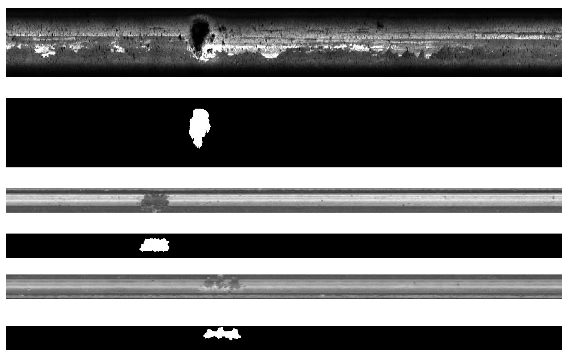
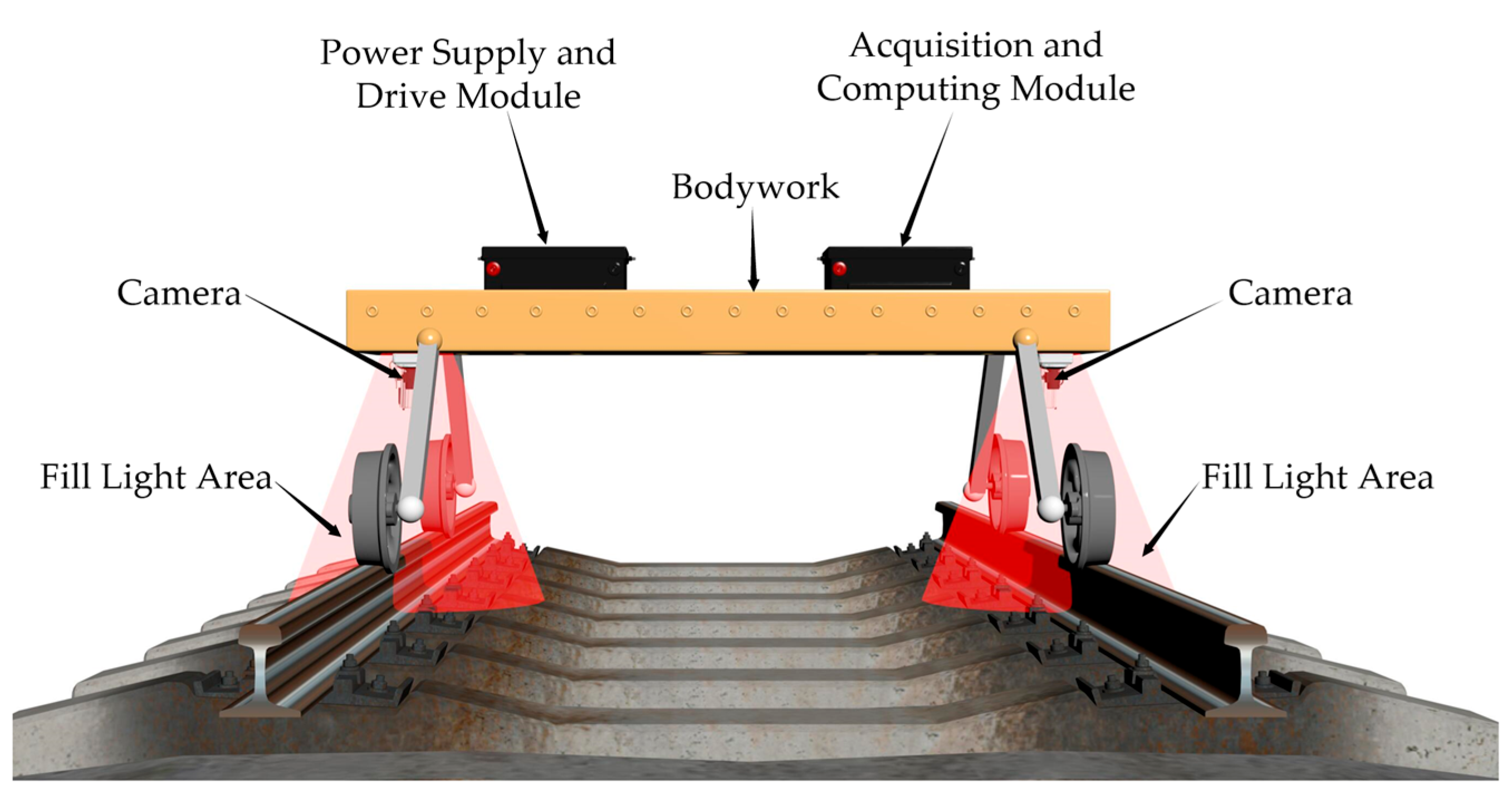
• In response to the public rail dataset, which is small and in black and white, this paper presents a comprehensive and colorful dataset of rail surface defects, derived from field photography, data tagging, and data expansion.
• Adding two Local Perception Modules (LPMs) to the Swin Transformer coding network improves segmentation accuracy by providing local context information.
• The decoding network now includes the Multiscale Feature Fusion Module (MFFM), which effectively fuses feature information of defects at different scales during the decoding process. This results in improved accuracy of multiscale defect segmentation.
• The decoding network now includes the Spatial Detail Extraction Module (SDEM), which preserves spatial detail information and enhances the segmentation accuracy of small-scale defects.

2. Materials and Methods

Figure 1 shows the Rail-STrans network framework, which assumes an encoder–decoder structure. The encoder is on the left, and the decoder is on the right. The Local Perception Module (LPM) is added to each stage of the Swin Transformer network in the encoder to enhance the network’s ability to acquire contextual information. The decoder comprises the Multiscale Feature Fusion Module (MFFM) and the Spatial Detail Extraction Module (SDEM). These modules efficiently fuse feature information from different scales of defects and preserve spatial detail information during the decoding process.

2.1. Dataset

Deep learning techniques are driven by data and learn from various scenarios to create a complete model for a specific task. Therefore, the performance of deep learning is limited by the size and accuracy of the dataset. There are limited publicly available datasets of rail surface defect images. The most commonly used dataset is the Rail Surface Defect Dataset (RSDDs). It includes two types of defect images captured from the rails of high-speed trains (67 images) and ordinary express and heavy transportation trains (128 images). Figure 2 shows the RSDDs dataset used as a training dataset for the network.

The RSDDs dataset consists of only 195 black-and-white images, which is insufficient for training the network model. The rail defects identified and localized by the semantic segmentation network lack intuitive presentation compared to color images. In this paper, we obtained 545 images of defects on the rail surface by shooting in the field of a specific section. The images were obtained with the support of relevant departments. The images were subjected to various forms of data expansion, including horizontal and vertical flipping, as well as rotation. This process generated 4500 rail surface defect images, of which 70% were used for training, 20% for testing, and 10% for validation. The resulting dataset is large-scale and colorful, and it was collected in strict adherence to national confidentiality laws and regulations. Due to the presence of national secrets in the dataset, its use is restricted, and it will not be released to the public. Part of the self-constructed dataset is shown in Figure 3.

2.2. Local Perception Module (LPM)

The camera-captured images contain valuable information about edges, contours, and textures. Therefore, this paper proposes using an improved Swin Transformer [47]-based feature extraction network to effectively extract rich contextual and long-term dependent information from the images. Figure 4 illustrates the structure of the improved Swin Transformer network.

The network framework comprises a Patch Partition module and four cascaded layers that output four feature maps with varying resolutions in stages. The Patch Partition module is used to chunk the image, while the first layer contains a Linear Embedding layer, two Local Perception Modules (LPMs), and two Swin Transformer modules. The initial layer of the four cascaded layers consists of a Linear Embedding layer, two Local Perception Modules (LPMs), and two Swin Transformer modules. The Linear Embedding layer is utilized to modify the number of channels in the feature map. The subsequent layers consist of a Patch Merging layer, an even number of LPMs, and an even number of Swin Transformer modules. The Patch Merging layer downsamples the spatial resolution by 2-fold to reduce the feature resolution and adjust the number of channels.

The Swin Transformer network framework has been improved by utilizing an even number of cascaded Swin Transformer modules. This allows for the division and merging of the surface defect feature map, thus expanding the local receptive field to the global receptive field. The network framework consists of four levels, each with different-resolution output feature maps, S1, S2, S3, and S4, which are $\frac{H}{4}\times \frac{H}{4}$, $\frac{H}{8}\times \frac{H}{8}$, $\frac{H}{16}\times \frac{H}{16}$, and $\frac{H}{32}\times \frac{H}{32}$, respectively. These output feature maps have varying receptive fields, ranging from small to large, which aids in the segmentation of defect targets of different scales.

The LPM framework, shown in Figure 5, obtains local context information of the image and reduces the number of network parameters. First, a set of feature vectors are reshaped into a spatial feature map using Reshape. Then, residual operations are performed on the outputs of DepthWise Separable Convolution (DWSC) and the SiLU activation module. Finally, the feature map is reduced to its original dimensions and output to the Swin Transformer module.

Figure 6 shows the structure of the Swin Transformer module, which comprises Window Multi-head Self-Attention (W-MSA), Shift Window Multi-head Self-Attention (SW-MSA), and Multilayer Perceptron (MLP), each with Layer Normalization (LN).

LN is used to normalize the features in order to make the training process more stable; meanwhile, in order to reduce the computational complexity, the W-MSA module confines the computation of the self-attention to a single window, and the output of its $l$th level is

$${\widehat{z}}^l=\mathit{W-MSA}\left(LN\left(z^{l-1}\right)\right)+z^{l-1}$$

(1)

And the output of the MLP layer at level l is

$${\widehat{z}}^l=MLP\left(LN\left({\widehat{z}}^l\right)\right)+{\widehat{z}}^l$$

(2)

In the next cascade module, SW-MSA adds a shift operation to W-MSA. This establishes information interaction between different windows without increasing computational effort. The output is as follows:

$${\widehat{z}}^{l+1}=\mathit{SW-MSA}\left(LN\left(z^l\right)\right)+z^l$$

(3)

$$z^{l+1}=MLP\left(LN\left({\widehat{z}}^{l+1}\right)\right)+{\widehat{z}}^{l+1}$$

(4)

where ${\widehat{z}}^{l+1}$ represents the output of the SW-MSA module at level $l+1$ and $z^{l+1}$ represents the output of the MLP module at level $l+1$.

In accordance with the methodology outlined in Equation (5), the W-MSA is calculated in a manner analogous to that of the SW-MSA.

$$\mathsf{\Omega }\left(\mathit{W-MSA}\right)=4hw{C}^2+2M^{2}hwC$$

(5)

The dimensions of the feature map, represented by the variables $h$, $w$, and $C$, respectively, are defined in terms of the size of each window, denoted by the variable $M$.

2.3. Multiscale Feature Fusion Module (MFFM)

To improve the accuracy of multiscale defect detection, this subsection proposes designing an MFFM to effectively fuse feature information from defects of different scales during the decoding process. The composition of the MFFM is shown in Figure 7.

In this module, the feature map with a resolution of 1/32 that is output from the improved Swin Transformer coding model is up-sampled using bilinear interpolation and then combined with the feature map with a resolution of 1/16 to obtain the feature map $f_a$. To enhance the model’s sensory field and integrate multiscale contextual information from different levels, this paper proposes constructing an atrous spatial pyramid pooling module. The module is designed to avoid the grid effect caused by atrous convolution by adding atrous convolution operations with different atrous rates in different channels. The loss of information is reduced by adding cross-layer jump connections. To ensure that the pixel points of the feature maps cover the entire input feature maps with a resolution of 1/16, the atrous rates are set as 1, 3, and 5. The outputs of its layers are shown in Equation (6).

$$F_a^i=\left\{\begin{array}{l}Conv\left(f_a\right),j=1\\ D_{3,1}\left(f_a\right),j=2\\ D_{3,3}\left(D_{3,1}\left(f_a\right)+F_a^2\right),j=3\\ D_{3,5}\left(D_{3,3}\left(D_{3,1}\left(f_a\right)+F_a^3\right)\right),j=4\\ Upsample\left(Pooling\left(f_a\right)\right),j=5\end{array}\right.$$

(6)

where $D_{f,d}$ represents the atrous convolution with convolution kernel $f$ and atrous ratio $d$.

Based on the analysis above, the MFFM presented in this paper can expand the model’s sensory field, fuse multiscale contextual information at different levels, and restore low-level detail and location information, high-level semantic information, and global contextual information. This improves the accuracy of multiscale defect segmentation.

2.4. Spatial Detail Extraction Module (SDEM)

As the image undergoes multiple downsampling operations in the encoder model, spatial detail information is gradually lost, resulting in poor detection of small-scale defects. To improve the segmentation accuracy of small-scale defects, this paper introduces SDEM, as shown in Figure 8.

SDEM consists of two parallel downsampling modules, each of which consists of a standard convolution layer with a step size of 2 and a maximum pooling layer. The input characteristic map of the downsampling module has a resolution of $H^{\prime }\times W^{\prime }\times {C_{in}}^{\prime }$, while the output characteristic map has a resolution of $\frac{H^{\prime }}{2}\times \frac{W^{\prime }}{2}\times {C_{out}}^{\prime }$. The number of input channels is represented by ${C_{in}}^{\prime }$, and the number of output channels is represented by ${C_{out}}^{\prime }$.

Based on the analysis presented above, the SDEM proposed in this paper can capture more detailed spatial information, thereby enhancing the accuracy of small-scale defect segmentation.

2.5. Loss Function and Evaluation Metrics

This paper utilizes dice loss as the loss function and evaluates model performance using accuracy, dice coefficient, and FPS metrics. Among these, accuracy and dice coefficient are closely related to the confusion matrix, as shown in Figure 9.

True Positive (TP) indicates that a sample is predicted to be a positive class and the true label is positive. False Positive (FP) indicates that a sample is predicted to be a positive case but the true label is a counterexample. False Negative (FN) indicates that a sample is predicted to be a counterexample but the true label is a positive case. True Negative (TN) indicates that a sample is predicted to be a counterexample and the true label is a counterexample.

Based on the confusion matrix, the accuracy formula can be given as

$$Accuracy=\frac{TP+TN}{TP+FP+FN+TN}$$

(7)

The dice coefficient is a similarity measure commonly used to calculate the similarity of two samples with a value threshold of [0, 1]. The highest possible segmentation result is 1, while the lowest is 0. The best result of segmentation is 1, and the worst result is 0. The calculation formula of the dice coefficient is shown in Equation (8).

$$Dice=\frac{2\times P}{\mathit{FP}+2\times \mathit{TP}+\mathit{FN}}$$

(8)

The dice loss function calculates the overlap between predicted and real results and minimizes the difference between the two to optimize the model. Its calculation formula is shown in Equation (9). Compared to the cross-entropy loss function, dice loss handles category imbalance better by considering the weight of each pixel in its calculation, rather than just using the number of pixels as weights. The dice loss function is a preferred choice for dealing with this type of task due to its objectivity and effectiveness. This paper’s self-constructed dataset is also an example of an unbalanced dataset, making the dice loss function a suitable choice for the training process of the network.

$$Dice Loss=1-\frac{2\times \mathit{TP}}{\mathit{FP}+2\times \mathit{TP}+\mathit{FN}}$$

(9)

3. Results

The algorithm model developed in this paper will be implemented on the platform of the railroad track inspection car, as illustrated in Figure 10 in the frames for the railroad inspection car. The platform comprises a camera, a light source, an acquisition and calculation module, a power supply, a drive module, and other components. The platform employs the light source to provide supplementary illumination to the rail surface below the railroad track inspection vehicle, and it captures an image of the rail surface damage through the camera and transmits the image to the acquisition and calculation module. Subsequently, the module loads the algorithm model designed in this paper and performs segmentation calculations on the acquired image. The final output is the result of the segmented rail surface damage. Railroad workers can rapidly identify the rail surface damage using this result.

3.1. Experimental Environment

The method proposed in this paper was implemented using the Pytorch 1.3 framework and Python language. All experiments and tests were conducted on NVIDIA Tesla P40 GPU (24G RAM, Single-Precision Performance is 12 TeraFLOPS) running on the Windows 10 operating system. During the training phase, the initial learning rate was set to 0.001, and the Adam algorithm was used for learning, with a weight decay factor of 0.0005 and a learning rate decay by cosine annealing. During model training, the preprocessing step uniformly adjusts the image size to 224 × 224. Figure 11 shows the training graph of the loss function, which stabilizes after 300 epochs.

3.2. Experimental Results and Analysis

3.2.1. Ablation Experiments

This paper conducts a series of ablation experiments to demonstrate the effectiveness of the proposed algorithm. The experiments verify the important role that each module plays in the algorithm’s improvement, including the LPM, MFFM, and SDEM modules.

Table 1. Results of the comparison of ablation experiment modules.

Model	Model Size/M	mAcc/%	mDice Coefficient/%	Background Acc/%	Defect Acc/%	Background Dice Coefficient/%	Defect Dice Coefficient/%
swin_upernet	701	85.04	72.31	99.27	70.81	99.55	45.07
swin_upernet + LPM	701	85.13	84.36	99.44	70.82	99.62	69.10
Swin Transformer + SDEM	508	87.56	87.41	99.45	75.67	99.54	75.28
Swin Transformer + MFFM	556	86.44	85.11	99.43	73.45	99.56	70.66
Swin Transformer + LPM + SDEM	508	88.02	87.56	99.51	76.53	99.64	75.48
Swin Transformer + MFFM + SDEM	357	88.54	88.32	99.52	77.56	99.58	77.06
Swin Transformer + LPM + MFFM	556	86.98	87.62	99.32	74.64	99.63	75.61
Rail-STrans	357	90.1	89.5	99.42	80.78	99.54	79.46

presents the experimental results for each module and their respective combinations. The data table lists various network configurations and their corresponding evaluation metrics, such as Params Size, mAcc (mean accuracy), mDice (mean dice coefficient), background accuracy, defect accuracy, background dice, and defect dice. The original swin_upernet is an encoder with Swin Transformer as the backbone network and UPerNet [48] as the encoder–decoder network.

The ablation experiment results demonstrate the significance of the MFFM (Multiscale Feature Fusion Module), SDEM (Spatial Detail Extraction Module), and LPM (Local Perception Module). By replacing the decoding network in the original swin_upernet with the SDEM and MFFM and forming an encoder–decoder semantic segmentation network with the Swin Transformer network alone, the model size can be effectively reduced while improving the mAcc and mDice coefficients.

The MFFM is a feature fusion module that aids the model in capturing features at various scales. This is essential for semantic segmentation tasks that necessitate precise identification and localization of defect boundaries in an image. The data show that Swin Transformer + MFFM enhances mAcc from 85.04% to 86.44% compared to the base swin_upernet. Additionally, it significantly improves the defect dice coefficients from 45.07% to 70.66%. This suggests that the MFFM has a positive impact on the model’s performance, particularly in capturing details.

The SDEM concentrates on extracting spatial details, which is essential for enhancing the segmentation accuracy of the model in complex scenes. The experimental results indicate that the addition of the SDEM significantly improved the model’s mAcc from 86.44% to 88.54% and its mDice coefficient from 85.11% to 88.32%, on average by 3%. This suggests that the SDEM enhances the model’s ability to understand detailed information in the image.

The LPM aims to improve the model’s local perception ability, which is crucial for recognizing and processing local changes in images. Based on the provided data, it appears that the addition of the LPM does not improve mAcc, but it does significantly improve the defect dice coefficient from 45.07% to 69.10%. This improvement is even more pronounced when used with the SDEM and MFFM, indicating that the LPM plays a role in the model’s local detail perception.

Finally, Rail-STrans achieves the best performance by combining three modules: the MFFM, SDEM, and LPM. The MFFM and SDEM significantly improve the model’s performance, while the LPM has a relatively small impact and may require further optimization or tuning to fully exploit its potential role. This paper proposes a model with a small number of parameters (357 M) and achieves mAcc and mDice of 90.1% and 89.5%, respectively. These results are significantly better than those of the underlying Swin Transformer network. This suggests that Rail-STrans achieves better overall performance while maintaining a smaller number of parameters. Figure 12 shows some pictures of ablation experiments.

3.2.2. Comparison Experiments

To evaluate the effectiveness of the improved algorithm, this paper compares it with other models, including deeplabv3+ [49], segnext_mscan [50], U-Net, Swin Transformer, SegFormer [51], and Mask R-CNN+ [22], which were trained on the same dataset. The results of the comparison are presented in

Table 2. Results of comparative experiments.

Model	Model Size/M	mAcc/%	mDice Coefficient/%	Background Acc/%	Defect Acc/%	Background Dice Coefficient/%	Defect Dice Coefficient/%	FPS
deeplabV3+	340	68.96	72.79	99.48	38.44	99.15	46.43	30.56
segnext_mscan	150	84.54	70.21	99.37	69.7	99.59	40.84	35.43
U-Net	118	53.4	55.72	96.54	10.26	96.21	15.32	39.36
swin_upernet	701	86.76	81.21	98.82	74.69	99.17	63.26	33.87
SegFormer	961	80.96	83.27	99.55	62.37	99.42	67.12	16.31
Mask R-CNN+	225	87.37	86.66	99.85	74.87	99.44	73.88	39.01
Rail-STrans	357	90.1	89.5	99.42	80.78	99.54	79.46	37.83

.

To analyze the advantages of Rail-STrans, we compare the performance of Rail-STrans with other networks on several metrics. Based on the data in Table 2, Rail-STrans shows advantages in the following aspects:

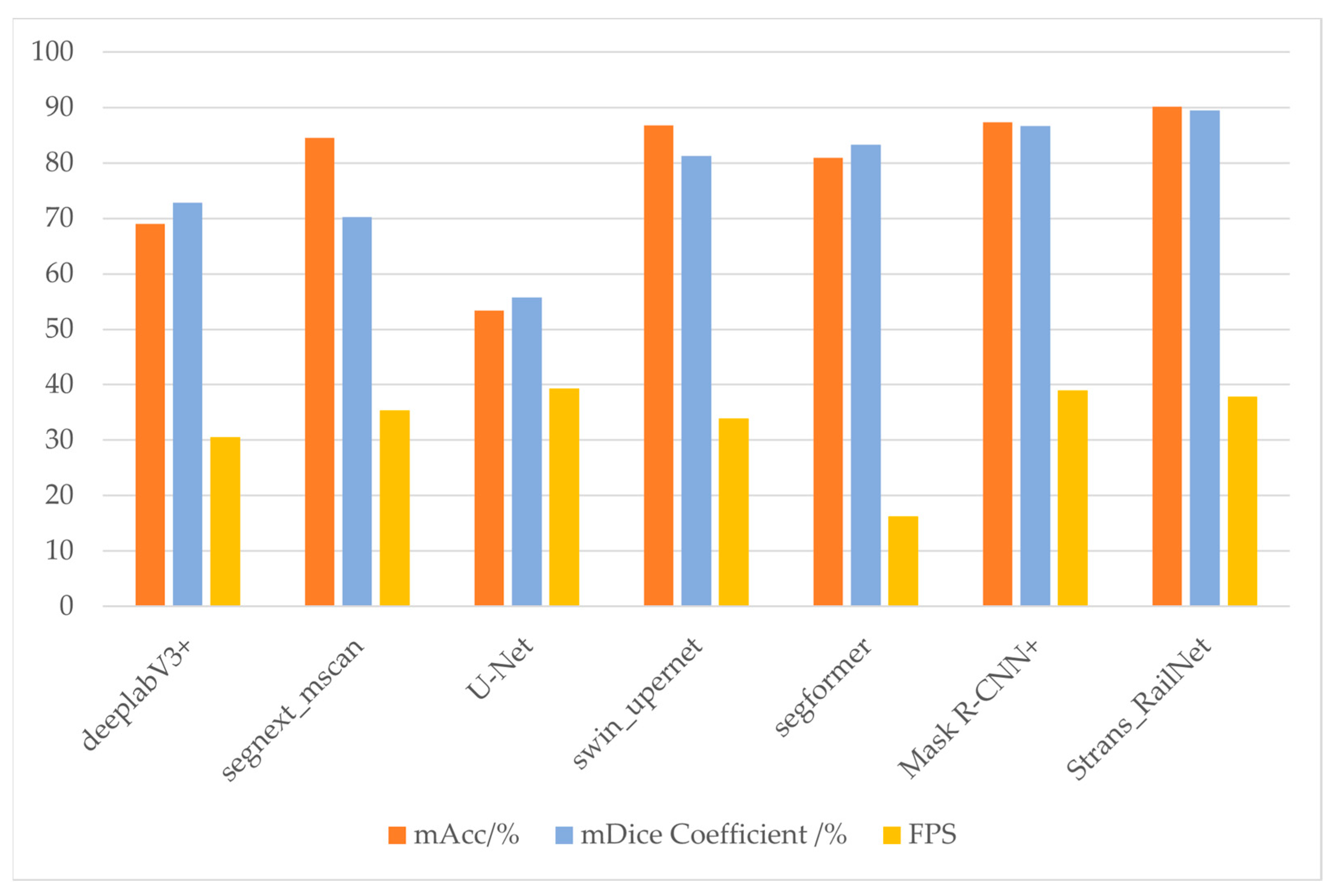
• Model size: The model size of Rail-STrans is 357 M, which is slightly larger than deeplabV3+, larger than segnext_mscan, U-Net, and swin_upernet, and much smaller than SegFormer. The model size of Rail-STrans is moderate, which is larger than some lightweight networks, such as U-Net, but much smaller than SegFormer, which is much smaller, suggesting that it has some model compression advantages while maintaining high performance.
• mAcc (mean accuracy): Rail-STrans has the highest average accuracy of 90.1%, which means it has the best overall classification performance.
• mDice (mean dice) coefficient: Rail-STrans also has the highest average dice coefficient of 89.5%, indicating that it outperforms the other networks in terms of pixel-level segmentation accuracy.
• Defect accuracy and defect dice coefficient: In terms of defect segmentation, Rail-STrans has a defect accuracy of 80.78% and a defect dice coefficient of 79.46%, which is also relatively good and sometimes second only to SegFormer.
• Background accuracy and background dice coefficient: Rail-STrans performs very well in background classification and segmentation, with a background accuracy of 99.42% and a background dice coefficient of 99.54%, both of which are the highest among all networks.
• FPS (Frames Per Second): Although Rail-STrans does not have the highest FPS, it is still able to provide processing speeds in excess of 37 FPS, which is acceptable for many real-time applications.

Figure 13 shows the combined data of deeplabv3+, segnext_mscan, U-Net, Swin Transformer, SegFormer, and Mask R-CNN+ in terms of mAcc, mDice coefficient, FPS, and so on. It can be seen that Rail-STrans shows significant advantages in several key performance metrics, especially in average accuracy and average dice coefficient, as well as in the accuracy of background classification and segmentation. These features make Rail-STrans a powerful and effective semantic segmentation network. Finally, our Rail-STrans model achieves an mAcc of 90.1% and an mDice coefficient of 89.5% with a medium number of parameters (357 M), which is the highest among all compared networks. This shows its superior performance in image segmentation tasks. Although Rail-STrans does not have the highest FPS, it is still able to provide processing speeds in excess of 30 FPS, which is acceptable for many real-time applications.

In summary, we can conclude that the model proposed in this paper (Rail-STrans) achieves the highest mAcc and mDice coefficient while maintaining a moderate number of parameters, and it is also fast and performs well. Therefore, in summary, compared with the current mainstream segmentation detection algorithms, the Rail-STrans algorithm proposed in this paper is effective in the task of rail surface defect segmentation detection.

To visually verify the effectiveness of the proposed model, we show a comparison of the visualized detection results of different models, as shown in Figure 14.

4. Conclusions

This study presents Rail-STrans, an encoder–decoder model based on an improved Swin Transformer network, to address the challenges of intelligent segmentation of surface defects on high-speed rail in complex scenarios. The proposed method is effective for the problem posed by non-equilibrium small datasets characterized by diversity and scale variability. The effectiveness of Rail-STrans is verified through a series of experiments and comparisons with other classical semantic segmentation methods. To begin with, we addressed the challenge of a limited black-and-white rail dataset by creating a larger and more diverse dataset of rail surface defects through field photography, data labeling, and data expansion. This approach not only provides ample data resources for future research but also ensures the adequacy and accuracy of model training. Secondly, we incorporated two Local Perception Modules (LPMs) into the Swin Transformer coding network. This enhancement allows for the acquisition of local contextual information, thereby improving segmentation accuracy. Our experimental results clearly demonstrate this improvement. Additionally, we integrated the Multiscale Feature Fusion Module (MFFM) into the decoding network. This module combines the feature information of defects at different scales during the decoding process, resulting in a significant improvement in the accuracy of multiscale defect segmentation. Additionally, we incorporated the Spatial Detail Extraction Module (SDEM) into the decoding network to preserve spatial detail information, further enhancing the segmentation accuracy of small-scale defects. Finally, we conducted ablation experiments to verify the function and role of each module. Our method outperforms other classical state-of-the-art networks in terms of mAcc, mDice coefficients, and FPS. It is a comprehensive improvement over other networks. Our research addresses the challenges of small datasets and variable defect scales in intelligent surface defect detection on high-speed rail. Additionally, we propose a new and effective semantic segmentation method. These findings have significant implications for high-speed rail maintenance and related research.

References

1. Jessop, C.; Ahlstrom, J.; Hammar, L.; Faester, S.; Danielsen, H.K. 3D Characterization of Rolling Contact Fatigue Crack Networks. Wear 2016, 366, 392–400. [Google Scholar] [CrossRef]
2. Molodova, M.; Li, Z.; Nunez, A.; Dollevoet, R. Automatic Detection of Squats in Railway Infrastructure. IEEE Trans. Intell. Transp. Syst. 2014, 15, 1980–1990. [Google Scholar] [CrossRef]
3. Kou, L. A Review of Research on Detection and Evaluation of the Rail Surface Defects. Acta Polytech. Hung. 2022, 19, 167–186. [Google Scholar] [CrossRef]
4. Xiong, Z.; Li, Q.; Mao, Q.; Zou, Q. A 3D Laser Profiling System for Rail Surface Defect Detection. Sensors 2017, 17, 1791. [Google Scholar] [CrossRef] [PubMed]
5. Cao, X.; Xie, W.; Ahmed, S.M.; Li, C.R. Defect Detection Method for Rail Surface Based on Line-Structured Light. Measurement 2020, 159, 107771. [Google Scholar] [CrossRef]
6. Liu, Z.; Li, W.; Xue, F.; Xiafang, J.; Bu, B.; Yi, Z. Electromagnetic Tomography Rail Defect Inspection. IEEE Trans. Magn. 2015, 51, 6201907. [Google Scholar] [CrossRef]
7. Fan, C.; Li, H.; Yan, B.; Sun, Y.; He, T.; Huang, T.; Yan, Z.; Sun, Q. High-Precision Distributed Detection of Rail Defects by Tracking the Acoustic Propagation Waves. Opt. Express 2022, 30, 39283–39293. [Google Scholar] [CrossRef] [PubMed]
8. Kundu, T.; Datta, A.K.; Topdar, P.; Sengupta, S. Optimal Location of Acoustic Emission Sensors for Detecting Rail Damage. Proc. Inst. Civ. Eng.-Struct. Build. 2022, 177, 254–263. [Google Scholar] [CrossRef]
9. Li, Q.; Ren, S. A Real-Time Visual Inspection System for Discrete Surface Defects of Rail Heads. IEEE Trans. Instrum. Meas. 2012, 61, 2189–2199. [Google Scholar] [CrossRef]
10. Dubey, A.K.; Jaffery, Z.A. Maximally Stable Extremal Region Marking-Based Railway Track Surface Defect Sensing. IEEE Sens. J. 2016, 16, 9047–9052. [Google Scholar] [CrossRef]
11. Yuan, X.; Wu, L.; Chen, H. Rail Image Segmentation Based on Otsu Threshold Method. Opt. Precis. Eng. 2016, 24, 1772–1781. [Google Scholar] [CrossRef]
12. He, Z.; Wang, Y.; Mao, J.; Yin, F. Research on Inverse P-M Diffusion-Based Rail Surface Defect Detection. Acta Autom. Sin. 2014, 40, 1667–1679. [Google Scholar]
13. Shi, T.; Kong, J.; Wang, X.; Liu, Z.; Zheng, G. Improved Sobel Algorithm for Defect Detection of Rail Surfaces with Enhanced Efficiency and Accuracy. J. Cent. South Univ. 2016, 23, 2867–2875. [Google Scholar] [CrossRef]
14. He, Z.; Wang, Y.; Liu, J.; Yin, F. Background Differencing-Based High-Speed Rail Surface Defect Image Segmentation. Chin. J. Sci. Instrum. 2016, 37, 640–649. [Google Scholar] [CrossRef]
15. Liu, Q.; Zhou, H.; Wang, X. Research on Rail Surface Defect Detection Method Based on Gray Equalization Model Combined with Gabor Filter. Surf. Technol. 2018, 19, 745–755. [Google Scholar]
16. Wang, H.; Wang, M.; Zhang, H.; Liu, G. Vision Saliency Detection of Rail Surface Defects Based on PCA Model and Color Features. Process Autom. Instrum. 2017, 38, 73–76. [Google Scholar] [CrossRef]
17. Kaewunruen, S.; Sresakoolchai, J.; Stittle, H. Machine Learning to Identify Dynamic Properties of Railway Track Components. Int. J. Struct. Stab. Dyn. 2022, 22, 2250109. [Google Scholar] [CrossRef]
18. Sresakoolchai, J.; Kaewunruen, S. Railway Defect Detection Based on Track Geometry Using Supervised and Unsupervised Machine Learning. Struct. Health Monit.-Int. J. 2022, 21, 1757–1767. [Google Scholar] [CrossRef]
19. Zhang, Z.; Che, X.; Song, Y. An Improved Convolutional Neural Network for Convenient Rail Damage Detection. Front. Energy Res. 2022, 10, 1007188. [Google Scholar] [CrossRef]
20. Li, Q.; Yuan, X.; Li, Y.; Zhu, Z. Rail Base Flaw Detection and Quantification Based on the Modal Curvature Method and the Back Propagation Neural Network. Eng. Fail. Anal. 2022, 142, 106792. [Google Scholar] [CrossRef]
21. Liu, W.; Tang, Z.; Lv, F.; Chen, X. An Efficient Approach for Guided Wave Structural Monitoring of Switch Rails Via Deep Convolutional Neural Network-Based Transfer Learning. Meas. Sci. Technol. 2023, 34, 024004. [Google Scholar] [CrossRef]
22. Zheng, D.; Li, L.; Zheng, S.; Chai, X.; Zhao, S.; Tong, Q.; Wang, J.; Guo, L. A Defect Detection Method for Rail Surface and Fasteners Based on Deep Convolutional Neural Network. Comput. Intell. Neurosci. 2021, 2021, 2565500. [Google Scholar] [CrossRef] [PubMed]
23. Kou, L.; Sysyn, M.; Fischer, S.; Liu, J.; Nabochenko, O. Optical Rail Surface Crack Detection Method Based on Semantic Segmentation Replacement for Magnetic Particle Inspection. Sensors 2022, 22, 8214. [Google Scholar] [CrossRef] [PubMed]
24. He, Z.; Ge, S.; He, Y.; Liu, J.; An, X. An Improved Feature Pyramid Network and Metric Learning Approach for Rail Surface Defect Detection. Appl. Sci. 2023, 13, 6047. [Google Scholar] [CrossRef]
25. Shelhamer, E.; Long, J.; Darrell, T. Fully Convolutional Networks for Semantic Segmentation. arXiv 2016, arXiv:1605.06211. [Google Scholar] [CrossRef]
26. Badrinarayanan, V.; Kendall, A.; Cipolla, R. SegNet: A Deep Convolutional Encoder-Decoder Architecture for Image Segmentation. IEEE Trans. Pattern Anal. Mach. Intell. 2017, 39, 2481–2495. [Google Scholar] [CrossRef] [PubMed]
27. Chen, L.-C.; Papandreou, G.; Kokkinos, I.; Murphy, K.; Yuille, A.L. Semantic Image Segmentation with Deep Convolutional Nets and Fully Connected CRFs. arXiv 2016, arXiv:1412.7062. [Google Scholar]
28. Ronneberger, O.; Fischer, P.; Brox, T. U-Net: Convolutional Networks for Biomedical Image Segmentation. arXiv 2015, arXiv:1505.04597. [Google Scholar]
29. Wang, Y.; Sun, Z.; Zhao, W. Encoder- and Decoder-Based Networks Using Multiscale Feature Fusion and Nonlocal Block for Remote Sensing Image Semantic Segmentation. IEEE Geosci. Remote Sens. Lett. 2021, 18, 1159–1163. [Google Scholar] [CrossRef]
30. Hu, X.; Jing, L.; Sehar, U. Joint Pyramid Attention Network For Real-Time Semantic Segmentation of Urban Scenes. Appl. Intell. 2022, 52, 580–594. [Google Scholar] [CrossRef]
31. Gu, Y.; Hao, J.; Chen, B.; Deng, H. Top-Down Pyramid Fusion Network for High-Resolution Remote Sensing Semantic Segmentation. Remote Sens. 2021, 13, 4159. [Google Scholar] [CrossRef]
32. Xiao, B.; Xu, B.; Bi, X.; Li, W. Global-Feature Encoding U-Net (GEU-Net) for Multi-Focus Image Fusion. IEEE Trans. Image Process. 2021, 30, 163–175. [Google Scholar] [CrossRef] [PubMed]
33. Zhang, Q.; Cong, R.; Li, C.; Cheng, M.; Fang, Y.; Cao, X.; Zhao, Y.; Kwong, S. Dense Attention Fluid Network for Salient Object Detection in Optical Remote Sensing Images. IEEE Trans. Image Process. 2021, 30, 1305–1317. [Google Scholar] [CrossRef] [PubMed]
34. Dong, H.; Song, K.; Wang, Y.; Yan, Y.; Jiang, P. Automatic Inspection and Evaluation System for Pavement Distress. IEEE Trans. Intell. Transp. Syst. 2022, 23, 12377–12387. [Google Scholar] [CrossRef]
35. Chen, L.; Xu, X.; Pan, L.; Cao, J.; Li, X. Real-Time Lane Detection Model Based on Non Bottleneck Skip Residual Connections and Attention Pyramids. PLoS ONE 2021, 16, e0252755. [Google Scholar] [CrossRef] [PubMed]
36. Cui, Z.; Lei, Y.; Wang, Y.; Yang, W.; Qi, J. Hand Gesture Segmentation against Complex Background Based on Improved Atrous Spatial Pyramid Pooling. J. Ambient Intell. Humaniz. Comput. 2022, 14, 11795–11807. [Google Scholar] [CrossRef]
37. Chen, B.; Tan, W.; Coatrieux, G.; Zheng, Y.; Shi, Y.Q. A Serial Image Copy-Move Forgery Localization Scheme with Source/Target Distinguishment. IEEE Trans. Multimed. 2021, 23, 3506–3517. [Google Scholar] [CrossRef]
38. Wu, Y.; Jiang, J.; Huang, Z.; Tian, Y. FPANet: Feature Pyramid Aggregation Network For Real-Time Semantic Segmentation. Appl. Intell. 2022, 52, 3319–3336. [Google Scholar] [CrossRef]
39. Liao, Y.; Liu, Q. Multi-Level and Multi-Scale Feature Aggregation Network for Semantic Segmentation in Vehicle-Mounted Scenes. Sensors 2021, 21, 3270. [Google Scholar] [CrossRef]
40. Lin, Z.; Sun, W.; Tang, B.; Li, J.; Yao, X.; Li, Y. Semantic Segmentation Network with Multi-Path Structure, Attention Reweighting and Multi-Scale Encoding. Vis. Comput. 2023, 39, 597–608. [Google Scholar] [CrossRef]
41. Wang, W.; Wang, S.; Li, Y.; Jin, Y. Adaptive Multi-Scale Dual Attention Network for Semantic Segmentation. Neurocomputing 2021, 460, 39–49. [Google Scholar] [CrossRef]
42. Zhang, X.; Du, B.; Wu, Z.; Wan, T. LAANet: Lightweight Attention-Guided Asymmetric Network for Real-Time Semantic Segmentation. Neural Comput. Appl. 2022, 34, 3573–3587. [Google Scholar] [CrossRef]
43. Vaswani, A.; Shazeer, N.; Parmar, N.; Uszkoreit, J.; Jones, L.; Gomez, A.N.; Kaiser, L.; Polosukhin, I. Attention is All You Need. arXiv 2017, arXiv:1706.03762. [Google Scholar]
44. Parmar, N.; Vaswani, A.; Uszkoreit, J.; Kaiser, L.; Shazeer, N.; Ku, A.; Tran, D. Image Transformer. arXiv 2018, arXiv:1802.05751. [Google Scholar]
45. Dosovitskiy, A.; Beyer, L.; Kolesnikov, A.; Weissenborn, D.; Zhai, X.; Unterthiner, T.; Dehghani, M.; Minderer, M.; Heigold, G.; Gelly, S.; et al. An Image is Worth 16x16 Words: Transformers for Image Recognition at Scale. arXiv 2021, arXiv:2010.11929. [Google Scholar]
46. Zheng, S.; Lu, J.; Zhao, H.; Zhu, X.; Luo, Z.; Wang, Y.; Fu, Y.; Feng, J.; Xiang, T.; Torr, P.H.; et al. Rethinking Semantic Segmentation from a Sequence-to-Sequence Perspective with Transformers. arXiv 2021, arXiv:2012.15840. [Google Scholar]
47. Liu, Z.; Lin, Y.; Cao, Y.; Hu, H.; Wei, Y.; Zhang, Z.; Lin, S.; Guo, B. Swin Transformer: Hierarchical Vision Transformer Using Shifted Windows. arXiv 2021, arXiv:2103.14030. [Google Scholar]
48. Xiao, T.; Liu, Y.; Zhou, B.; Jiang, Y.; Sun, J. Unified Perceptual Parsing for Scene Understanding. arXiv 2018, arXiv:1807.10221. [Google Scholar]
49. Chen, L.-C.; Zhu, Y.; Papandreou, G.; Schroff, F.; Adam, H. Encoder-Decoder with Atrous Separable Convolution for Semantic Image Segmentation. In Computer Vision—ECCV 2018; Lecture Notes in Computer Science; Springer: Cham, Switzerland, 2018; pp. 833–851. [Google Scholar]
50. Guo, M.-H.; Lu, C.-Z.; Hou, Q.; Liu, Z.-N.; Cheng, M.-M.; Hu, S.-M. SegNeXt: Rethinking Convolutional Attention Design for Semantic Segmentation. arXiv 2022, arXiv:2209.0857. [Google Scholar]
51. Xie, E.; Wang, W.; Yu, Z.; Anandkumar, A.; Alvarez, J.; Luo, P. SegFormer: Simple and Efficient Design for Semantic Segmentation with Transformers. arXiv 2021, arXiv:2105.15203. [Google Scholar]
Figure 1. Rail-STrans network framework.
Applsci 14 03629 g001
Figure 2. Rail surface defect image from the RSDDs dataset.
Applsci 14 03629 g002
Figure 3. Dataset built in this paper. (a) Original picture. (b) Flip 45 degrees. (c) Flip horizontal. (d) Flip vertical.
Applsci 14 03629 g003aApplsci 14 03629 g003b
Figure 4. Improved Swin Transformer network structure diagram.
Applsci 14 03629 g004
Figure 5. LPM framework.
Applsci 14 03629 g005
Figure 6. The architecture of the Swin Transformer block.
Applsci 14 03629 g006
Figure 7. The architecture of MFFM.
Applsci 14 03629 g007
Figure 8. The architecture of SDEM. (a) SDEM; (b) the structure of DM.
Applsci 14 03629 g008
Figure 9. Confusion matrix.
Applsci 14 03629 g009
Figure 10. Frames for railroad inspection car.
Applsci 14 03629 g010
Figure 11. The training curve of loss function.
Applsci 14 03629 g011
Figure 12. Partial picture display of ablation experiments. (a) Original picture; (b) swin_upernet; (c) swin_upernet + LPM; (d) Swin Transformer + SDEM; (e) Swin Transformer + MFFM; (f) Swin Transformer + LPM + SDEM; (g) Swin Transformer + MFFM + SDEM; (h) Swin Transformer + LPM + MFFM; (i) Rail-STrans.
Applsci 14 03629 g012aApplsci 14 03629 g012b
Figure 13. Performance comparison of different segmentation models.
Applsci 14 03629 g013
Figure 14. The visual segmentation results of different models. (a) Original picture; (b) deeplabV3+; (c) segnext_mscan; (d) U-Net; (e) swin_upernet; (f) SegFormer; (g) Mask R-CNN+; (h) Rail-STrans.
Applsci 14 03629 g014