Optimization of Pickup Vehicle Scheduling for Steel Logistics Park with Mixed Storage

Abstract

Pickup vehicle scheduling in steel logistics parks is an important problem for determining the outbound efficiency of steel products. In a steel logistics park, each yard contains different types of steel products, which provides flexible yard selection for each pickup operation. In this case, the yard allocation and the loading sequence for each vehicle must be considered simultaneously in pickup vehicle scheduling, which greatly increases the scheduling complexity. To overcome this challenge, in this paper, we propose a pickup vehicle scheduling problem with mixed steel storage (PVSP-MSS) to optimize the makespan of pickup vehicles and the makespan of steel logistics parks simultaneously. The optimization problem is formulated as a multi-objective mixed-integer linear programming model, and an enhanced algorithm based on SPEA2 (ESPEA) is proposed to solve the problem with a high efficiency. In the ESPEA, a cooperative initialization strategy is firstly proposed to initialize the vehicle pickup sequence for each yard. Then, an insertion decoding method is designed to improve the scheduling efficiency, utilizing the idle time of a yard. Furthermore, local search technology based on critical paths is proposed for the ESPEA to improve the solution quality. Experiments are executed based on data collected from a real steel logistics park. The results confirm that the ESPEA can significantly reduce both the makespan of each pickup vehicle and the makespan of the steel logistics park.

1. Introduction

Pickup vehicle scheduling is important for steel logistics parks, and can greatly reduce the waiting time of vehicles and improve the logistics throughput [1,2]. On the other hand, optimizing vehicle scheduling in the industrial or logistics field is also an important way to reduce $\mathrm{C}{\mathrm{O}}_2$ emissions [3,4]. Traditionally, pickup vehicles are manually scheduled, which is inefficient and always leads to scheduling conflicts since it is too complex to be efficiently scheduled by humans [5,6]. Therefore, it is essential to develop an automatic pickup vehicle scheduling algorithm based on the data of pickup vehicles to improve the outbound efficiency of steel logistics parks.

In recent years, some strategies have been developed to improve the efficiency of vehicle scheduling. Kulkani et al. (2018) in [7] proposed a timetabled assignment for the multi-warehouse vehicle scheduling problem and designed a formula for the temporal-spatial network flow and solved it using the column generation algorithm. Wang et al. (2021) in [8] proposed a path optimization problem for pickup vehicles in warehouses and designed a mathematical model and a double-layer coding genetic algorithm to solve the problem. Priscila et al. (2022) in [9] proposed an integrated problem of pickup vehicle scheduling and route decision making to reduce the delay time of service customers in multiple docks and designed a mixed-integer linear programming model and two heuristic methods to solve the problem. Wang et al. (2020) in [10] proposed a dynamic bus vehicle scheduling approach to efficiently generate scheduling solutions, addressing the problem of traffic congestion. Liao (2020) in [11] proposed a newly formulated model and a hybrid optimization method for solving the integrated vehicle routing and scheduling problem in a multi-door cross-dock terminal. Yağmur and Kesen (2021) in [12] addressed a joint production scheduling and outbound distribution planning problem, considering a permutation flow shop setting and multiple heterogeneous capacitated vehicles. The objective is to minimize the total tour time of the vehicles while considering the tardiness resulting from late deliveries.

However, the aforementioned studies did not consider the vehicle scheduling problem in the steel logistics field. To solve the pickup vehicle scheduling problem in steel logistics parks, Wen et al. (2022) in [13] proposed a constrained clustering of vehicle batching algorithm, which optimized the sequence of vehicles entering a steel logistics park and the selection of the operation yard to minimize the makespan. Tang et al. (2009) in [14] considered a pickup vehicle and trailer vehicle scheduling problem and developed an inherited tabu search algorithm to solve the problem. Kunnapapdeelert and Thawnern (2021) in [15] addressed the capacitated vehicle routing problem in the steel industry by utilizing Clarke and Wright’s saving algorithm.

These works provide inspiration for solving the pickup vehicle scheduling problem for steel logistics parks. However, they are not applicable to pickup vehicle scheduling in a steel logistics park with mixed storage. In a steel logistics park, each yard contains different types of steel products [16], which provides the flexible yard selection for each pickup operation. In this case, the yard allocation and the loading sequence for each vehicle must be considered simultaneously in pickup vehicle scheduling, which significantly increases the complexity of the problem.

To cope with these problems, in this paper, we propose to optimize the pickup vehicle scheduling problem with mixed steel storage (PVSP-MSS) based on the data of pickup vehicles collected by the IIoT. Firstly, a multi-objective mixed-integer linear programming model is formulated to describe the PVSP-MSS. Then, an enhanced algorithm based on SPEA2 (ESPEA) is proposed to solve the problem with a high efficiency.

Specifically, this paper has the following contributions:

• The pickup vehicle scheduling problem with mixed steel storage (PVSP-MSS) is investigated in this paper. The PVSP-MSS is formulated as a multi-objective mixed-integer linear programming model, aiming at simultaneously optimizing the makespan of pickup vehicles and the makespan of the steel logistics park. By solving this problem, the optimal yard allocation and loading sequence for vehicles can be obtained.
• The ESPEA is proposed to solve the PVSP-MSS with a high efficiency. In the proposed algorithm, a cooperative initialization strategy is first proposed to provide an initial solution for scheduling optimization. Then, insertion decoding is designed to optimize the quality of the solution by utilizing the idle time in the yard. Moreover, local search technology is proposed in the ESPEA to improve the solution quality by swapping pickup operations on critical paths in steel logistics parks.
• The experiments are executed based on the data from a real steel logistics park. The results show that compared with other algorithms, the proposed algorithm significantly reduces both the makespan of each pickup vehicle and the makespan of the steel logistics park.

The rest of this paper is organized as follows. Section 2 introduce the framework of scheduling based on IIoT and the data features of pickup vehicles. An optimization model is formulated in Section 3. Section 4 proposes an ESPEA to solve the proposed problem. Section 5 discusses the experiment results, and the conclusion is given in Section 6.

2. Scheduling Framework and Pickup Vehicle Data

This section introduces the framework of pickup vehicle scheduling in a steel logistics park based on the Industrial Internet of Things (IIoT) to depict how to achieve vehicle scheduling in the cloud environment. In addition, in order to facilitate the elaboration of problem characteristics, the data of vehicles in the cloud platform are introduced in detail.

2.1. Scheduling Framework Based on the IIoT

A cloud platform represents a valuable tool for widely sharing manufacturing services and solutions by connecting suppliers and customers in large-scale manufacturing networks [17,18]. Figure 1 shows the framework of scheduling based on the IIoT in a steel company. The IIoT collects data from vehicles and uploads them to the platform. Based on these data, the cloud platform allocates resources for each pickup vehicle operation. It is worth noting that each yard stores mixed steels ans thus contains a variety of different types of steel, which allows pickup vehicles to obtain target goods from different yards. The goal of scheduling is to allocate the most appropriate yard for each vehicle and determine the optimal operation sequence for individual vehicles, both of which are considered in this paper. The results of scheduling generate the decision for the vehicle operation sequence and the yard allocation. Therefore, scheduling is important to increase the efficiency of vehicles and the throughput of the park.

2.2. Data of Pickup Vehicles

The data in this paper are based on pickup data from a real steel logistics park. Each pickup vehicle has 13 attributes, including vehicle number, customer ID, steel category, operation number, delivery date, etc. Figure 2 shows the statistics of the pickup vehicle numbers over a month, where the star represents the number of vehicles. There are 1695 vehicles in total, and the number of pickup vehicles each day is distributed between 10 and 100. The number of steel types picked up for each vehicle is between 1 and 4.

Base on the data given above, we formulate a pickup vehicle scheduling model, and the details are given in the following sections.

3. Pickup Vehicle Scheduling Model

In this section, the pickup vehicle scheduling problem with mixed steel storage (PVSP-MSS) is formulated as a multi-objective mixed-integer linear programming model (MILP). This model can accurately describe the processes of pickup vehicles in a steel logistics park.

3.1. Assumptions

For the construction of the model, in this study, the following assumptions are made.

• All vehicles have the same priority.
• All vehicles and yards are available at the start time of the steel logistics park.
• Interruptions during each operation do not occur.
• The transition time of vehicle operation is short and negligible.

3.2. Pickup Time Model

The pickup time plays a crucial role in allocating vehicles to the yard. The pickup time of the vehicle depends on the pick up time and movement time of the crane, as well as the number of corresponding pickup goods. Therefore, the vehicle pickup time t can be modeled as:

$$t=\left(\frac{2d_y}{v}+\alpha \right)N$$

(1)

where $d_y$ represents the distance between the storage location of the goods and the pickup port of the yard, v represents the speed of the crane, $\alpha$ represents the time taken for the crane to pick up one unit of goods, and N represents the number of goods. Due to the number of collected goods for each vehicle and the storage location of the goods in each yard being the variables to be determined, the pickup time of vehicles in each yard is fixed.

3.3. Variable Definitions

To depict the PVSP-MSS effectively, the parameters and decision variables involved in the optimization model are defined below.

(1)

Parameters

$n:$	Total number of vehicles.
m :	Total number of steel logistics park yards.
$I:$	Set of vehicles, where $I=\{1,2,\dots ,n\}$.
$M:$	Set of yards in the steel logistics park, where $M=\{1,2,\dots ,m\}$.
$i,i^{\prime }:$	Index of vehicles, where $i,i^{\prime }\in \{1,\dots ,n\}$.
$n_i:$	Number of operations of vehicles i.
$J_i$ :	Set of operations of vehicle i, where $J_i=\left\{1,2,\dots ,n_i\right\}$.
$j,j^{\prime }$ :	Index of operations of vehicles i, where $j,j^{\prime }\in \left\{1,\dots ,n_i\right\}$.
$k,k^{\prime }$ :	Index of yards, where $k,k^{\prime }\in \{1,\dots ,m\}$.
$O_{i,j}:$	The j operation of vehicle i.
$U_{i,j}$ :	Optional set of yards for j operations of vehicle i.
$S_{i,j}$ :	Start time of operation $O_{i,j}$.
$t_{i,j,k}$ :	Pickup time of operation $O_{i,j}$ at yard k.
$C_{i,j}$ :	Completion time of operation $O_{i,j}$.
$C_{max}$ :	Makespan of steel logistics park.
$S{C}_{max}$ :	Maximum makespan of all vehicles.
L :	A large number for maintaining the consistency of the inequality.

(2)

Decision Variables

$X_{i,j,k}$:	Takes a value of 1 if the operation $O_{i,j}$ is processed at yard k and 0 otherwise.
$y_{i,j,p,q,k}$:	Takes a value of 1 if the operation $O_{i,j}$ takes precedence over the operation $O_{p,q}$ at yard k and 0 otherwise.

3.4. Mathematical Model for the PVSP-MSS

This study presents the MILP model for the PVSP-MSS with two objective functions. The MILP model is described as follows:

$$\begin{array}{cc}\hfill & min{\mathbf{F}}_{\mathbf{1}}=C_{max}=max\{C_{i,n_i}\mid \forall i\in I\}\hfill \end{array}$$

(2)

$$\begin{array}{cc}\hfill & min{\mathbf{F}}_{\mathbf{2}}=S{C}_{max}=max\{C_{i,n_i}-S_{i,1}\mid \forall i\in I\}\hfill \end{array}$$

(3)

where ${\mathbf{F}}_{\mathbf{1}}$ indicates the minimization for the makespan of the steel logistics park and ${\mathbf{F}}_{\mathbf{2}}$ indicates the minimization for the maximum makespan of all vehicles. It is worth noting that ${\mathbf{F}}_{\mathbf{1}}$ has an implicit conflict with ${\mathbf{F}}_{\mathbf{2}}$. In other words, blindly reducing ${\mathbf{F}}_{\mathbf{2}}$ might lead to a sharp increase in ${\mathbf{F}}_{\mathbf{1}}$ and vice versa. Thus, the PVSP-MSS is multi-objective optimization problem subject to:

$$\begin{array}{cc}\hfill & S_{i,j}+t_{i,j,k}+L\left(X_{i,j,k}-1\right)\le C_{i,j},\forall i\in I,j\in J_i\hfill \end{array}$$

(4)

$$\begin{array}{cc}\hfill & C_{i,j}\le S_{i,j+1},\forall i\in I,j\in \left\{1,\dots ,n_i-1\right\}\hfill \end{array}$$

(5)

$$\begin{array}{cc}\hfill & S_{p,q}\ge S_{i,j}+t_{i,j,k}-L(3-y_{i,j,p,q,k}-X_{i,j,k}-X_{p,q,k}),\hfill \\ \hfill & \forall i\in I,j\in J_i,p\in I,q\in J_p,k\in U_{i,j}\cap U_{p,q}\hfill \end{array}$$

(6)

$$\begin{array}{cc}\hfill & S_{i,j}\ge S_{p,q}+t_{i,j,k}+L(2+y_{i,j,p,q,k}-X_{i,j,k}-X_{p,q,k}),\hfill \\ \hfill & \forall i\in I,j\in J_i,p\in I,q\in J_p,k\in U_{i,j}\cap U_{p,q}\hfill \end{array}$$

(7)

$$\begin{array}{cc}\hfill & \sum _{k=1}^{U_{i,j}}{X}_{i,j,k}=1,\forall i\in I,j\in J_i\hfill \end{array}$$

(8)

$$\begin{array}{cc}\hfill & S_{i,j}\ge 0,\forall i\in I,j\in J_i\hfill \end{array}$$

(9)

$$\begin{array}{cc}\hfill & t_{i,j,k}\ge 0,\forall i\in I,j\in J_i,k\in U_{i,j}\hfill \end{array}$$

(10)

$$\begin{array}{cc}\hfill & C_{i,j}\ge 0,\forall i\in I,j\in J_i\hfill \end{array}$$

(11)

Constraint (4) ensures that the completion time of vehicle operations is greater than or equal to the sum of the start time of operations and the pickup time. Constraint (5) ensures that start time of the next operation is greater than or equal to the completion time of the current operation. Constraints (6) and (7) ensure that a yard can only serve one vehicle at a time. Constraint (8) ensures that each vehicle operation can only be a pickup operation in one optional yard at a time. Constraints (9)–(11) are value range limitations.

The model is a typical mixed-integer linear programming model with NP-hard characteristics. To test the proposed model, GUROBI 10.0.1 based on the python programming language is implemented to solve some instances. The experiments in Section 5 show that the complexity of the problem is so high that GUROBI cannot find an optimal solution in the desired time.

4. ESPEA for Solving the PVSP-MSS

The PVSP-MSS is a complex problem in the pickup vehicle scheduling process. In order to improve the scheduling efficiency, each vehicle can flexibly select a yard according to its needs, which greatly increases the scheduling complexity and makes it difficult for the existing algorithms to obtain high-quality solutions within a reasonable time. Therefore, this paper proposes an enhanced algorithm based on SPEA2 [19] to solve the PVSP-MSS. Firstly, a cooperative initialization strategy is proposed, which utilizes the pickup vehicle sequence and pickup time in different yards to provide an initial solution for the optimal schedule. Secondly, to optimize the quality of the solution, an insertion decoding method is proposed to effectively utilize the idle time in the yard. Finally, local search technology is proposed in the ESPEA to improve the solution quality by swapping pickup operations on critical paths in the steel logistics park.

4.1. Framework of the ESPEA

In this subsection, the proposed algorithm is outlined in Algorithm 1. In steps S1–S2, we encode a pickup vehicle arrangement scheme using two one-dimensional sequences and further use the cooperative initialization strategy to provide an initial solution for the optimal schedule. In step S3, a null elite archive is created to store elite individuals. During the population evolution process, steps S4–S6 utilize insertion decoding to optimize the pickup vehicle sequence. Then, the objective value and the fitness value for each individual are calculated. Based on the fitness value, steps S7–S8 use the population environment to select elite individuals for crossover and mutation. In step S9, a local search technique based on the critical path is used to find a better scheduling solution.

Algorithm 1 Framework of the ESPEA

Input: Initial number of iterations $q=0$; maximum number of iterations $q_{max}$; near neighbor threshold k; elite archive size $\eta$; population size $NP$, crossover probability $CP$, mutation probability $MP$; Output: Pareto front solution for the elite archive $A_{q_{max}}$;     S1: Particle coding for pickup vehicle arrangement scheme, go to S2;     S2: Generate population $P_0$ using the cooperative initialization strategy, go to S3;     S3: Create a null elite archive $A_0$, go to S4;     while $q<q_{max}$ do           S4: Insertion decoding for $P_q$ and $A_q$, go to S5;           S5: Calculate the object value according to (2) and (3) for $P_q$ and $A_q$, go to S6;           S6: Calculate the fitness F according to (15) for $P_q$ and $A_q$, go to S7;           S7: Select environment for $P_q$ and $A_q$, and save the elite individual to $A_{q+1}$, go to S8;           S8: Crossover and mutation for $A_{q+1}$, and save the results to $P_{q+1}$, go to S9;           S9: Local search based on a critical path for $P_{q+1}$ to generate new solution, and replace the parent solution as much as possible, go to S10;           S10: Update q = q + 1;     end while

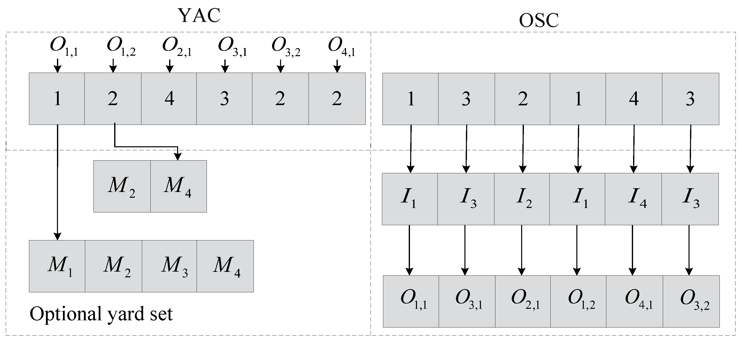
4.2. Particle Coding for Pickup Vehicle Arrangement

For the pickup vehicle arrangement scheme, two one-dimensional integer sequence codings are picked to encode particles. An operation sequence chain (OSC) is used to represent the sequence of vehicle operations and its length is equal to the total number of vehicle operations. In the OSC, each gene is directly encoded by the vehicle index; the position where the vehicle index appears indicates the sequence of operations for that vehicle. The yard allocation chain (YAC) is used to allocate a yard for each vehicle operation and its length is equal to the length of the OSC. Each gene of the YAC is arranged according to the vehicle index and vehicle operation sequence, and each integer represents the serial number of the yard currently allocated to the operation in the set of optional yards.

Figure 3 displays an instance of chromosome encoding, where the OSC is [1, 3, 2, 1, 4, 3] and the the YAC is [1, 2, 4, 3, 2, 2]. In the YAC, all operations of vehicle $I_1$ to vehicle $I_4$ are arranged in sequence. Operation $O_{1,1}$ has four optional yards, and the corresponding ‘1’ represents the first yard $M_1$ in the set of optional yards. Similarly, operation $O_{1,2}$ has two optional yards, which is yard $M_2$ and yard $M_4$, respectively. The corresponding ‘2’ represents the second yard in the optional yards, which is yard $M_4$. In the OSC, the first ‘1’ represents operation $O_{1,1}$ of vehicle $I_1$, and the second ‘3’ represents operation $O_{3,1}$ of vehicle $I_3$ and so on; the operation sequence of each vehicle is $O_{1,1}\to O_{3,1}\to O_{2,1}\to O_{1,2}\to O_{4,1}\to O_{3,2}$.

4.3. Cooperative Initialization Strategy

In order to improve the throughput of the steel logistics park and the scheduling efficiency of pickup vehicles, a cooperative initialization strategy that uses the pickup vehicle sequence and the pickup time in different yards is proposed to provide an initial solution for scheduling optimization.

The cooperative initialization strategy used in this paper includes three initialization mechanisms that have different effects on the optimization, and their details are depicted in the following.

4.3.1. YWB

YWB refers to yard workload balancing mechanism, which is designed to balance the workload of a yard to increase the throughput of the steel logistics park. In the procedure of YWB, we first encode the OSC based on vehicle data and shuffle the encoded sequence. Then, we allocate the yard with the minimum workload to each vehicle operation. The procedure of YWB is shown in Algorithm 2.

An example of YWB is shown in Figure 4. It is assumed there are two vehicles and each vehicle has two operations. According to S1 and S2, assume the OSC is [1, 2, 2, 1]; for each operation, allocate the yard that has the minimum value from the temporary array (indicated by a red box). Finally, the yards $[M_1,M_2,M_3,M_4]$ are accordingly allocated for $[O_{1,1},O_{2,1},O_{2,2},O_{1,2}]$ and the YAC is [1, 4, 2, 3].

Algorithm 2 Procedure of YWB

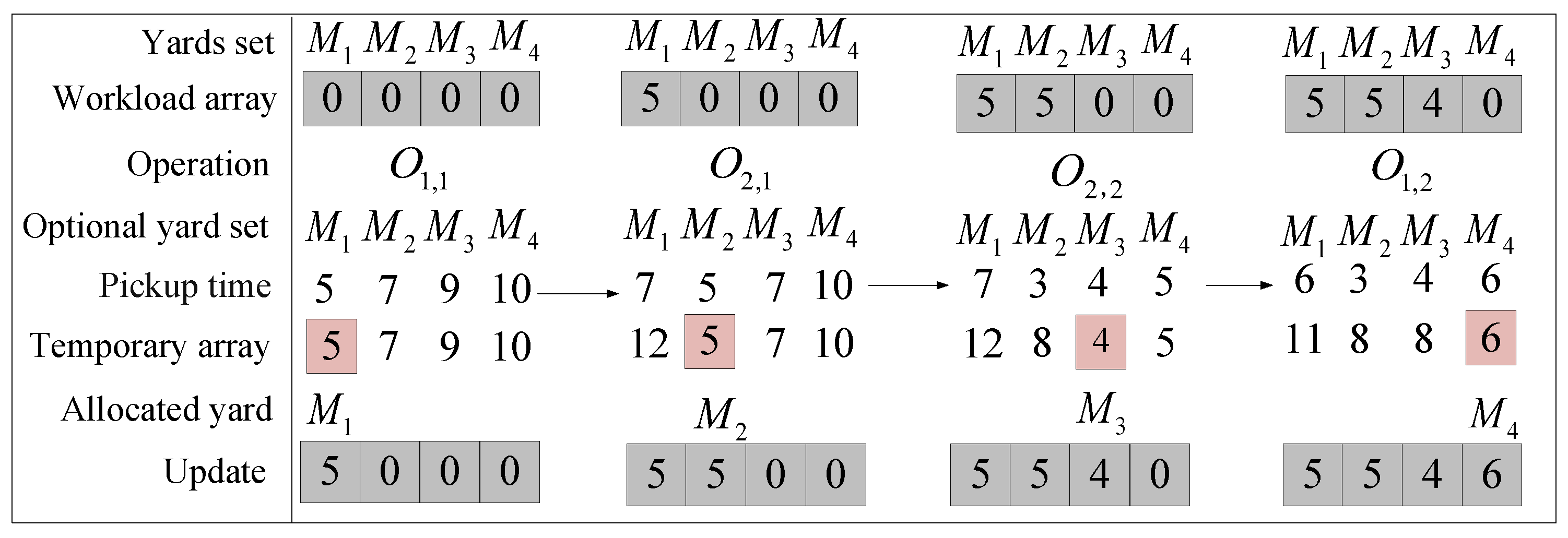
S1: Encode for OSC based on vehicle data, go to S2; S2: Shuffle the OSC, go to S3; S3: Initialize workload array with all elements set to zero, go to S4; for O in OSC do      S4: According to the optional yard set of O, add the pickup time to the workload array and save it in the temporary array, go to S5;      S5: Allocate the minimum workload yard to O, and set the corresponding gene of YAC to the yard (if there are multiple yards with the same minimum value, allocate the yard with the minimum pickup time), go to S6;      S6: Update the workload array; end for S7: Output OSC and YAC;

4.3.2. MPT

MPT refers to minimum pickup time mechanism, which is designed to allocate the yard with the minimum pickup time to vehicles to improve the efficiency of pickup vehicles. In the procedure of MPT, we first encode the OSC based on vehicle data and shuffle the encoded sequence. Then, we allocate the yard with the minimum pickup time to each vehicle operation. The procedure of MPT is shown in Algorithm 3.

Algorithm 3 Procedure of MPT

S1: Encode for the OSC based on vehicle data, go to S2; S2: Shuffle the OSC, go to S3; for O in the OSC do      S3: Allocate minimum pickup time to O in the optional yard, and set the corresponding gene of the YAC to the allocated yard (if there are multiple yards with the same minimum processing time, then one of them is randomly allocated); end for S4: Output the OSC and YAC;

4.3.3. RVS

RVS refers to the random vehicle sequential mechanism, which is designed to increase the diversity of vehicle scheduling schemes. The procedure of RVS is very similar to that of MPT, except that in S3, optional yards are randomly allocated to vehicles.

In solving the PVSP-MSS, the population is cooperatively initialized by YWB, MPT, and RVS in equal proportions.

4.4. Insertion Decoding

During the operation of the steel logistics park, a redundant yard idle time will affect the logistics efficiency. In this paper, an insertion decoding method is designed to insert vehicle operations into the idle time of a yard to sufficiently utilize the idle time of the yard if it meets the insertion conditions of the operation. This subsection will elucidate the implementation details of insertion decoding.

4.4.1. Decoding the YAC

The YAC can be converted into a yard allocation matrix $Y_m[j,h]$ and a time matrix $T[j,h]$, where $Y_m[j,h]$ indicates that the $h-th$ operation of the $I_j$ allocated yard and $T[j,h]$ indicates that the $h-th$ operation pickup time of $I_j$. It is worth noting that there is a one-to-one correspondence between $Y_m$ and T.

Taking Figure 3 as an example, the yard allocation chain is [1, 2, 4, 3, 2, 2]. The converted yard allocation matrix and time matrix are:

$$Y_m[j,h]=\left[\begin{array}{cc}1& 2\\ 4\\ 3& 2\\ 2\end{array}\right],T[j,h]=\left[\begin{array}{cc}5& 7\\ 8\\ 6& 4\\ 3\end{array}\right]$$

$Y_m[1,2]=2$ indicates the second operation of $I_1$ has been allocated to the second optional yard, which is $M_4$. Meanwhile, $T[1,2]=7$ indicates that the pickup time is 7 min for the second operation of $I_1$ at $M_4$.

4.4.2. Decoding the OSC

$Y_m$ and T are used to determine the corresponding yard $M_k$ and pickup time $t_{i,j,k}$. For vehicle operation $O_{i,j}$ and yard $M_k$, if $O_{i,j}$ is the first operation of vehicle i and the first operation of yard $M_k$, it can be inserted directly into the 0 moment for processing; if $O_{i,j}$ is the first operation of $M_k$ but not the first operation of vehicle i, $O_{i,j}$ can be inserted directly at the completion time of the previous operation $O_{i,j-1}$. Otherwise, find all idle time periods [$T{S}_x$, $T{E}_x$] for yard $M_k$, where $T{S}_x$ is the start time of the $x-th$ idle time period and $T{E}_x$ is the end time of the $x-th$ idle time period. During yard $M_k$’s work process, if $O_{i,j}$ satisfies the condition $max\{C_{i,j-1},T{S}_x\}+t_{i,j,k}\le T{E}_x$, it can be inserted into the idle time [$T{S}_x$, $T{E}_x$] with the start time of $\{C_{i,j-1},L{M}_k\}$, where $L{M}_k$ is the earliest available time for the current yard $M_k$.

Figure 5 shows an insertable example in $M_2$. $O_{4,1}$ is the first operation of $I_4$, and the pickup time $t_{4,1,2}$ is 3, which is less than the idle time period [$T{S}_1$,$T{E}_1$] of $M_2$. Therefore, $O_{4,1}$ can be inserted ahead of $O_{1,2}$ without affecting the normal operation of $I_1$.

Figure 6 shows a non-insertable example in $M_2$. $O_{3,2}$ is the second operation of $I_3$, and has $S_{3,2}\ge C_{3,1}\ge T{E}_1$. Therefore, $O_{3,2}$ cannot be inserted into the idle time of $M_2$ and it is assigned to the next operation after $O_{1,2}$.

4.5. Fitness Value

In the proposed ESPEA, the fitness value is calculated by considering both the raw fitness and the proximity density. The raw fitness is used to measure the superiority of individuals in the multi-objective function space and is determined by counting the number of times an individual is dominated by other individuals. A smaller raw fitness indicates a higher level of superiority in the objective space. On the other hand, the proximity density takes into account the distribution density of individuals in the population. It measures how crowded an individual is in its local region of the objective space. A smaller proximity density suggests a more even distribution of individuals.

In the iterative process, each individual i of population $P_q$ and elite archive $A_q$ is assigned a strength value $S\left(i\right)$, which is described as follows:

$$S\left(i\right)=\left|\{j\mid j\in P_q+A_q\wedge i\succ j\}\right|$$

(12)

Specifically, we first need to calculate the dominance relationship for each individual based on the object value. Then, the strength value $S\left(i\right)$ for individual i is calculated. Based on the value of $S\left(i\right)$, the raw fitness $R\left(i\right)$ of an individual i is calculated as follows:

$$R\left(i\right)=\sum _{j\in P_q+A_q,j\succ i}S\left(j\right)$$

(13)

When $R\left(i\right)$ = 0, this indicates that individual i is a non-dominated individual. The purpose of the algorithm is to find individuals with smaller $R\left(i\right)$ values and save them. However, most of the individuals do not dominate each other during the actual operation of the algorithm. Therefore, density information is introduced to distinguish individuals with the same original fitness value. The density $D\left(i\right)$ of individual i is defined as follows:

$$D\left(i\right)=\frac{1}{{\sigma }_i^k+2}$$

(14)

where ${\sigma }_i^k$ is the distance in the objective space between an individual i and the $k-$th adjacent individual. The parameter k is the near neighbor threshold, and adding two to ${\sigma }_i^k$ ensures that the range of values is within the interval $(0,1)$.

Finally, adding $D\left(i\right)$ to $R\left(i\right)$ calculates the fitness $F\left(i\right)$, as expressed as follows:

$$F\left(i\right)=R\left(i\right)+D\left(i\right)$$

(15)

4.6. Environment Selection

Environmental selection is the process of selecting elite individuals for the next generation in the process of evolution in order to select a good pickup vehicle scheduling scheme and thus accelerate algorithm convergence. During the selection process, the first step is to copy all non-dominated individuals in $P_q$ and $A_q$ to $A_{q+1}$, as expressed as follows:

$$A_{q+1}=\{x^i\mid x^i\in P_q\cup A_q\}$$

(16)

If the archived Pareto solution size of $A_{q+1}$ is over the elite archive size $\eta$, the size is reduced to $\eta$, but if the size of $A_{q+1}$ is less than $\eta$, the dominant solutions from $A_q$ and $P_q$ are added to $A_{q+1}$ until the size of $A_{q+1}$ is equal to $\eta$.

4.7. Crossover and Mutation

In the ESPEA, an elite archive preserves the outstanding individuals of the previous generation. The population diversity needs to be increased to prevent algorithms from falling into local optimization. Therefore, new population individuals need to be generated via crossovers and mutations from elite individuals.

4.7.1. Crossover Operator

For as much diversity as possible, precedence operation crossover [20] and two-point crossover [21] are applied to develop a crossover operator in the two one-dimensional integer sequence chains. The description is given in the following.

The process of precedence operation crossover for the vehicle operation sequence chain is as follows: (1) Randomly divide the vehicle set into two subsets $se{t}_1$ and $se{t}_2$. (2) Randomly select two solutions $S_1$ and $S_2$. For each vehicle belonging to $se{t}_1$, copy their operations into $New{S}_1$, and for each vehicle belonging to $se{t}_2$, copy their operations into $New{S}_2$. (3) For an empty space in $New{S}_1$ and $New{S}_2$, start from one side of S2 and copy the missing operation which does not appear in $New{S}_1$ to the vacant positions in $New{S}_1$ from left to right, and perform a similar operation for $New{S}_2$. An example of precedence operation crossover is illustrated in Figure 7.

The process of two-point crossover for the yard allocation chain is as follows: (1) Two gene sites are randomly selected in $S_1$ and $S_2$. (2) Mutual exchange of all genes between the two crossover points is performed to produce two new chromosomes: $New{S}_1$ and $New{S}_2$. The procedure is illustrated in Figure 8.

4.7.2. Mutation Operator

(1) Vehicle operation sequence chain mutation: randomly select two positions and exchange the value.

(2) Yard allocation chain mutation: randomly select two positions and choose one new yard from the optional yard set.

4.8. Local Search Based on Critical Paths

In this paper, we propose local search technology to improve the solution quality by swapping the pickup vehicle operations on the critical path in the steel logistics park.

The critical path directly affects the maximum completion time of scheduling; it is defined as the longest path of all paths from the start node to the end node and the operations in the critical path are defined as critical operations. Moving an operation on the critical path can optimize the current solution more efficiently [22]. In this paper, adjacent operations on the critical path in the same yard are called critical sets, and we design a critical path neighborhood structure based on the idea of critical operation movement. The detailed procedure of the local search technology based on critical paths is shown in Algorithm 4. In this local search technique, FindCriticalSetsOnCriticalPath() identifies all critical sets. LengthOfSet() determines the length of each set. As for LastTwoDiffVehicles(), if the last two critical operations belong to different vehicles, then LastTwoDiffVehicles() is true; otherwise, it is false. SwapLastTwoOps() represents swapping the last two critical operations. For FirstTwoDiffVehicles(), if the first two critical operations belong to different vehicles, then FirstTwoDiffVehicles() is true; otherwise, it is false. SwapFirstTwoOps() represents swapping the first two critical operations. An example of a local neighborhood based on the critical path is illustrated in Figure 9.

Algorithm 4 Local search based on critical paths

Input: Schedule S; Output: Improved schedule S’; $critical\_sets\leftarrow$ FindCriticalSetsOnCriticalPath(S); if LengthOfSet($set\left[0\right]$) > 1 then       if LastTwoDiffVehicles($critical\_sets\left[0\right]$) then             SwapLastTwoOps($critical\_sets\left[0\right]$)       end if end if if LengthOfSet($set[-1]$) > 1 then       if FirstTwoDiffVehicles($critical\_sets[-1]$) then             SwapFirstTwoOps($critical\_sets[-1]$)       end if end if for $set$ in $critical\_sets$ do       if LengthOfSet($set$) == 2 then             if FirstTwoDiffVehicles($set$) then                    SwapFirstTwoOps($set$)             end if       end if       if LengthOfSet($set$) $>=$ 4 then             if FirstTwoOpsDiffVehicles($set$) then                   SwapFirstTwoOps($set$)             end if             if LastTwoOpsDiffVehicles($set$) then                   SwapLastTwoOps($set$)             end if       end if end for Return $S^{\prime }$

5. Numerical Experiments

This section aims to prove the effectiveness of the proposed scheduling strategy through numerical experiments. The simulation experiments include the following aspects.

(1)

Validation of the proposed MILP model.

(2)

Effectiveness analysis of the improved strategies in the proposed ESPEA.

(3)

Comparison of the ESPEA with other multi-objective optimization algorithms on the PVSP-MSS.

All algorithms were coded in Python 3.9 and run on a computer with an Intel Core i5-12400 (2.5 GHz) and 32 GB RAM (Intel, Santa Clara, CA, USA).

5.1. Evaluation Metric

In this paper, we use $C_{max}$, $S{C}_{max}$, $CT\left(s\right)$ and the hypervolume ($HV$) [23] as the performance indicators. $C_{max}$ is the makespan of steel logistics park, which is defined in (2). $S{C}_{max}$ is the maximum makespan of all vehicles, which is defined in (3). $CT\left(s\right)$ is the running time of the algorithm and $HV$ is an evaluation indicator for multi-objective algorithms used to measure the quality of the solution, calculated as follows:

$$HV(P,r)=\bigcup _{x\in P}^{P}v(x,r)$$

(17)

where P is the Pareto frontier calculated by the algorithms, r is the reference point of the Pareto frontier and $r=(1,1)$. The non-dominant solution in the Pareto frontier needs to be normalized, which can be written as $x=\left(\frac{f_1}{f_{1max}},\frac{f_2}{f_{2max}}\right)$, where $f_{1max}$ and $f_{2max}$ are the ideal maximum values of the objective function for each problem scale. The larger the value of $HV$, the better the performance of the algorithm.

5.2. Test Data

In order to better verify the performance of the algorithm at different data scales, we select historic vehicle data from a real steel logistics park and extract the data of different vehicle quantities [10, 20, 30, 40, 50, 60, 70, 80, 90, 100]. The number of operations per vehicle is distributed between 1 and 4.

Table 1. Problem scales of the test data.

Index	Size
	Vehicle Number	Total Number of Operations
1	10	25
2	20	57
3	30	84
4	40	89
5	50	135
6	60	163
7	70	187
8	80	212
9	90	239
10	100	264

shows the total number of operations for all vehicles at different vehicle scales.

5.3. Validation of the Proposed MILP Model

In this experiment, we use six small-scale examples to validate the model and solve them using GUROBI 11.0 (the academic license is applied by Jinlong Wang from China) and ESPEA , where V/O/Y represents the number of vehicles, the number of operations for each vehicle, and the number of yards.

Table 2. Comparison results with the GUROBI solver on small scale of instances.

V/O/Y	GUROBI			ESPEA
	${\mathit{C}}_{\mathit{max}}$	${\mathit{SC}}_{\mathit{max}}$	$\mathit{CT}\mathbf{\left(}\mathit{s}\mathbf{\right)}$	${\mathit{C}}_{\mathit{max}}$	${\mathit{SC}}_{\mathit{max}}$	$\mathit{CT}\mathbf{\left(}\mathit{s}\mathbf{\right)}$
5/4/4	39	37	23.59	43	38	37.13
6/4/4	43	40	43,241	43	41	36.2
7/4/4	-	-	-	41	30	36.8
8/4/4	-	-	-	49	30	36.69
9/4/4	-	-	-	56	30	37.41
10/4/4	-	-	-	47	32	37.24

shows the comparison results with the GUROBI solver on a small scale of instances. Bold values represent the best results for the same metrics. As the test scale slightly increases, it can be seen that the time consumption of GUROBI increases exponentially. For the first two instances, GUROBI is slightly better than the ESPEA but the time consumption has increased 1800-fold, which is unacceptable in the application scenario. For the other instances, GUROBI cannot even find the optimal solution in the prescribed time; in contrast, the ESPEA can find feasible solutions in a short time.

5.4. Effectiveness Analysis of Each Improved Strategy

In order to verify the effectiveness of the proposed cooperative initialization strategy, insertion decoding method and local search technology based on critical paths, one ablation experiment was conducted. Specifically, three variants of the ESPEA are taken into account, namely ESPEA-1, ESPEA-2, and ESPEA-3. SPEA2 is the basic algorithm without any improvement, ESPEA-1 is SPEA2 with the cooperative initialization strategy, ESPEA-2 is ESPEA-1 with local search techniques based on critical paths, and ESPEA-3 is ESPEA-2 with insertion decoding. The $HV$ value of SPEA2 is used as a benchmark to evaluate the performance of the three versions of the ESPEA. To ensure fairness, all experiments were run 10 times. For the SPEA2 algorithm, “aver” represents the average value of the 10 experimental results, while “best” represents the best result among the 10 experiments. For the other three improved versions, “aver_gap” represents the improvement in each version’s average value relative to the average value of the 10 experiments of SPEA2, and “best_gap” represents the improvement relative to the best result among the 10 experiments. 

Table 3. Values of evaluation metrics for ESPEA variants.

Index	SPEA2		ESPEA-1		ESPEA-2		ESPEA-3
	aver	best	aver_gap	best_gap	aver_gap	best_gap	aver_gap	best_gap
1	0.54297521	0.557345	3.62%	3.06%	4.79%	3.06%	4.82%	3.06%
2	0.36817818	0.409204	14.87%	8.46%	17.06%	10.03%	19.94%	11.89%
3	0.35772439	0.380317	21.37%	20.68%	26.66%	23.26%	29.43%	26.36%
4	0.36172758	0.400679	17.41%	12.94%	22.50%	16.72%	25.56%	19.06%
5	0.33120254	0.35396	26.70%	24.87%	29.18%	24.62%	33.40%	30.81%
6	0.25820991	0.296639	37.35%	24.16%	41.45%	25.86%	47.79%	31.36%
7	0.22072806	0.248489	48.40%	35.68%	53.32%	41.78%	57.34%	44.66%
8	0.20389379	0.225313	57.08%	49.95%	59.15%	47.52%	64.47%	57.68%
9	0.21106804	0.224812	56.37%	49.36%	59.92%	52.98%	64.26%	58.99%
10	0.21625091	0.235104	53.35%	47.19%	56.03%	48.36%	61.94%	52.91%

shows the comparison results. Bold indicated the best result for each instance. As shown, for all test instances, each part improves the performance of the algorithm compared to the previous one; in particular, as the scale of the problem increases, the magnitude of the improvement becomes more pronounced. This proves the effectiveness of each improvement strategy.

5.5. Performance Analysis via an Algorithm Comparison

In order to better illustrate the performance of the proposed ESPEA, the performances of other excellent multi-objective algorithms are compared with that of the proposed algorithm. These comparison algorithms include ROMA/D [24], MOEA/D [25], SPEA2 [19], NSGAII [26] and NSGAIII [27], all of which have been proven to have an excellent performance. In order to fairly compare the solving ability of different algorithms, all algorithms used the same cooperative initialization strategy and genetic operators and all algorithms were run 10 independent times. These algorithms’ parameter settings are shown in

Table 4. Parameter settings.

Algorithm	Special Parameters	Common Parameters
ESPEA	Near neighbor threshold k = $\sqrt{200}$ Elite archive size $\eta$ = 100	Maximum iteration number $q_{max}$ = 100 Popsize size $NP$ = 100 Crossover rate $CP$ = 1 Mutation $MP$ = 0.8
RMOEA/D	Memory size LP = 40 Learning rate $\epsilon$ = 0.4 Discount rate $\gamma$ = 0.6 Greedy factor $\delta$ = 0.8 Neighborhood vector T = [5, 10, 15, 20] Vectors number = 100
MOEA/D	Neighborhood vector T = 20 Vector number = 100
NSGAII	None
NSGAIII	None
SPEA2	Near neighbor threshold k = $\sqrt{200}$ Elite archive size $\eta$ = 100

, and the results of $HV$ are given in

Table 5. $HV$ results for a comparison with other algorithms.

Index	ESPEA		RMOEA/D		MOEA/D		SPEA2		NSGAII		NSGAIII
	aver	best	aver	best	aver	best	aver	best	aver	best	aver	best
1	0.56913054	0.574422	0.559479	0.572862	0.556422	0.558821	0.562658	0.57438	0.568211	0.57438	0.564754	0.574212
2	0.44158741	0.457874	0.435142	0.441398	0.412667	0.4349381	0.422917	0.443818	0.422483	0.43538	0.419455	0.444849
3	0.46301166	0.480571	0.448158	0.467332	0.432563	0.4433533	0.434173	0.458972	0.432443	0.444264	0.442867	0.455924
4	0.45417245	0.477058	0.440325	0.455548	0.419309	0.432326	0.424721	0.452521	0.431632	0.442927	0.434009	0.445102
5	0.44181358	0.463014	0.589584	0.610275	0.410716	0.434287	0.419627	0.441983	0.419262	0.430315	0.417667	0.429318
6	0.3816034	0.389679	0.352019	0.372049	0.349841	0.3614302	0.354652	0.368318	0.354481	0.369025	0.354934	0.370934
7	0.34729293	0.359455	0.328926	0.346557	0.321556	0.3286682	0.327551	0.337147	0.327222	0.334943	0.324626	0.341105
8	0.33535407	0.355284	0.318119	0.336925	0.308004	0.3128554	0.320283	0.337848	0.317105	0.327807	0.3167	0.323428
9	0.34669923	0.357434	0.317965	0.336408	0.326519	0.339133	0.330039	0.335774	0.329104	0.338439	0.329755	0.34147
10	0.35019048	0.359495	0.323144	0.338917	0.328994	0.3369403	0.331614	0.346047	0.330904	0.344449	0.33791	0.348614

.

As shown in Table 5, it can be seen that the ESPEA is very competitive, obtaining the optimal values of the average $HV$ and the best $HV$ for different problem scales. It is worth noting that as the number of vehicles increases, the advantage of the ESPEA becomes increasingly prominent. This is because the local search technology based on critical paths in the ESPEA is more targeted than other local search technologies. This local search technology of swapping critical operations not only reduces the computational cost, but also optimizes the overall scheduling time. Additionally, the insertion decoding method adopted in the ESPEA effectively utilizes the idle time in the yard and improves the logistics efficiency. As the problem scale increases, the advantages of the local search based on critical paths and insertion decoding become more apparent.

Figure 10 shows the Pareto frontiers of the various comparison algorithms in instance 5. It can be seen that the Pareto frontier obtained by the ESPEA converges faster and is more diverse than other comparative algorithms. For the Pareto front obtained by the ESPEA, we can use the equivalent weight method to obtain the pickup vehicle scheduling scheme, as shown in Figure 11. In this scheme, the maximum makespan of all vehicles and the makespan of the steel logistics park of this scheme are [117, 225].

6. Conclusions

In this paper, we propose utilizing the data of vehicles collected from a real steel logistics park by the IIoT to optimize the pickup vehicle scheduling problem with mixed steel storage (PVSP-MSS). The PVSP-MSS is firstly formulated as a multi-objective mixed-integer linear programming model. Then, an enhanced algorithm based on SPEA2 is proposed to solve the optimization problem with a high efficiency. In the ESPEA, a cooperative initialization strategy is proposed to provide an initial solution for scheduling optimization. Moreover, an insertion decoding method is proposed to effectively utilize the idle time of a yard. Additionally, local search technology based on critical paths is proposed to improve the solution quality. The experimental results show that compared with other algorithms, the ESPEA can achieve better scheduling results.

This study effectively addresses the problem of cross-yard pickups in logistics scheduling in the steel industry and significantly improves the vehicle scheduling efficiency. However, this study does not consider the vehicle rescheduling problem in cases of vehicle delays and other exceptional situations. In future research, we will expand the model and develop more advanced algorithms to tackle more complex engineering scheduling problems.

References

1. Beham, A.; Raggl, S.; Hauder, V.A.; Karder, J.; Wagner, S.; Affenzeller, M. Performance, quality, and control in steel logistics 4.0. Procedia Manuf. 2020, 42, 429–433. [Google Scholar] [CrossRef]
2. Xu, Z.; Wang, J.; Yuan, M.; Yuan, Y.; Chen, B.; Zhang, Q.; Chen, C.; Guan, X. Joint optimization of steel plate shuffling and truck loading sequencing based on deep reinforcement learning. Adv. Eng. Inform. 2024, 60, 102392. [Google Scholar] [CrossRef]
3. Choi, J.; Xuelei, J.; Jeong, W. Optimizing the construction job site vehicle scheduling problem. Sustainability 2018, 10, 1381. [Google Scholar] [CrossRef]
4. Li, H.; Yuan, J.; Lv, T.; Chang, X. The two-echelon time-constrained vehicle routing problem in linehaul-delivery systems considering carbon dioxide emissions. Transp. Res. Part D Transp. Environ. 2016, 49, 231–245. [Google Scholar] [CrossRef]
5. Dong, C.; Wang, H.; Zhang, H.; Zhang, M.; Guan, J.; Zhang, Z.; Lin, Q.; Zuo, Z. Research on Fine Scheduling and Assembly Planning of Modular Integrated Building: A Case Study of the Baguang International Hotel Project. Buildings 2022, 12, 1892. [Google Scholar] [CrossRef]
6. Lim, A.; Zhang, Z.; Qin, H. Pickup and delivery service with manpower planning in Hong Kong public hospitals. Transp. Sci. 2017, 51, 688–705. [Google Scholar] [CrossRef]
7. Kulkarni, S.; Krishnamoorthy, M.; Ranade, A.; Ernst, A.T.; Patil, R. A new formulation and a column generation-based heuristic for the multiple depot vehicle scheduling problem. Transp. Res. Part B Methodol. 2018, 118, 457–487. [Google Scholar] [CrossRef]
8. Wang, C.L.; Wang, Y.; Zeng, Z.Y.; Lin, C.Y.; Yu, Q.L. Research on logistics distribution vehicle scheduling based on heuristic genetic algorithm. Complexity 2021, 2021, 1–8. [Google Scholar] [CrossRef]
9. Cota, P.M.; Nogueira, T.H.; Juan, A.A.; Ravetti, M.G. Integrating vehicle scheduling and open routing decisions in a cross-docking center with multiple docks. Comput. Ind. Eng. 2022, 164, 107869. [Google Scholar] [CrossRef]
10. Wang, C.; Shi, H.; Zuo, X. A multi-objective genetic algorithm based approach for dynamical bus vehicles scheduling under traffic congestion. Swarm Evol. Comput. 2020, 54, 100667. [Google Scholar] [CrossRef]
11. Liao, T.W. Integrated outbound vehicle routing and scheduling problem at a multi-door cross-dock terminal. IEEE Trans. Intell. Transp. Syst. 2020, 22, 5599–5612. [Google Scholar] [CrossRef]
12. Yağmur, E.; Kesen, S.E. Multi-trip heterogeneous vehicle routing problem coordinated with production scheduling: Memetic algorithm and simulated annealing approaches. Comput. Ind. Eng. 2021, 161, 107649. [Google Scholar] [CrossRef]
13. Wen, W.; Chen, K.; Wang, J.; Xu, Z.; Wang, R.; Chen, B.; Zhang, Q. Vehicle Scheduling for Steel Logistics Based on Vehicle Batching. In Proceedings of the 2022 IEEE International Conference on Industrial Technology (ICIT), Shanghai, China, 22–25 August 2022; IEEE: Piscataway, NJ, USA, 2022; pp. 1–6. [Google Scholar]
14. Tang, L.; Li, K. An Inherited Tabu Search Algorithm for the truck and trailer vehicle scheduling problem in iron and steel industry. ISIJ Int. 2009, 49, 51–57. [Google Scholar] [CrossRef]
15. Kunnapapdeelert, S.; Thawnern, C. Capacitated vehicle routing problem for Thailand’s steel industry via saving algorithms. J. Syst. Manag. Sci. 2021, 11, 171–181. [Google Scholar]
16. Pang, K.W.; Chan, H.L. Data mining-based algorithm for storage location assignment in a randomised warehouse. Int. J. Prod. Res. 2017, 55, 4035–4052. [Google Scholar] [CrossRef]
17. Wang, J.; Xu, Z.; Wen, W.; Wang, R.; Lin, Y.; Yuan, Y.; Chen, B.; Zhang, Q. Optimization for Storage Scheduling of Steel Plates Based on Cloud Manufacturing Platform. IEEE Trans. Ind. Inform. 2023, 19, 11653–11663. [Google Scholar] [CrossRef]
18. Simeone, A.; Zeng, Y.; Caggiano, A. Intelligent decision-making support system for manufacturing solution recommendation in a cloud framework. Int. J. Adv. Manuf. Technol. 2021, 112, 1035–1050. [Google Scholar] [CrossRef]
19. Zitzler, E.; Laumanns, M.; Thiele, L. SPEA2: Improving the strength Pareto evolutionary algorithm. TIK Rep. 2001, 103, 1–21. [Google Scholar]
20. Gao, K.Z.; Suganthan, P.N.; Chua, T.J.; Chong, C.S.; Cai, T.X.; Pan, Q.K. A two-stage artificial bee colony algorithm scheduling flexible job-shop scheduling problem with new job insertion. Expert Syst. Appl. 2015, 42, 7652–7663. [Google Scholar] [CrossRef]
21. Zhang, J.; Yang, J. Flexible job-shop scheduling with flexible workdays, preemption, overlapping in operations and satisfaction criteria: An industrial application. Int. J. Prod. Res. 2016, 54, 4894–4918. [Google Scholar] [CrossRef]
22. Doostali, S.; Babamir, S.M.; Eini, M. CP-PGWO: Multi-objective workflow scheduling for cloud computing using critical path. Clust. Comput. 2021, 24, 3607–3627. [Google Scholar] [CrossRef]
23. While, L.; Hingston, P.; Barone, L.; Huband, S. A faster algorithm for calculating hypervolume. IEEE Trans. Evol. Comput. 2006, 10, 29–38. [Google Scholar] [CrossRef]
24. Li, R.; Gong, W.; Lu, C. A reinforcement learning based RMOEA/D for bi-objective fuzzy flexible job shop scheduling. Expert Syst. Appl. 2022, 203, 117380. [Google Scholar] [CrossRef]
25. Zhang, Q.; Li, H. A multiobjective evolutionary algorithm based on decomposition. IEEE Trans. Evol. Comput. 2006, 11, 712–731. [Google Scholar] [CrossRef]
26. Deb, K.; Pratap, A.; Agarwal, S.; Meyarivan, T. A fast and elitist multiobjective genetic algorithm: NSGA-II. IEEE Trans. Evol. Comput. 2002, 6, 182–197. [Google Scholar] [CrossRef]
27. Deb, K.; Jain, H. An evolutionary many-objective optimization algorithm using reference-point-based nondominated sorting approach, part I: Solving problems with box constraints. IEEE Trans. Evol. Comput. 2013, 18, 577–601. [Google Scholar] [CrossRef]
Figure 1. The framework of pickup vehicle scheduling.
Applsci 14 03628 g001
Figure 2. Number of pickup vehicles.
Applsci 14 03628 g002
Figure 3. An instance of chromosome encoding.
Applsci 14 03628 g003
Figure 4. An example of YWB.
Applsci 14 03628 g004
Figure 5. An example of an insertable operation.
Applsci 14 03628 g005
Figure 6. An example of a non-insertable operation.
Applsci 14 03628 g006
Figure 7. An example of precedence operation crossover.
Applsci 14 03628 g007
Figure 8. An example of two-point crossover.
Applsci 14 03628 g008
Figure 9. An example of a local neighborhood based on the critical path.
Applsci 14 03628 g009
Figure 10. The Pareto frontier of all algorithms for instance 5.
Applsci 14 03628 g010
Figure 11. Pickup vehicle scheduling scheme.
Applsci 14 03628 g011