Article

Drive-by Bridge Damage Detection Using Continuous Wavelet Transform

by
Kultigin Demirlioglu
and
Emrah Erduran
*
Department of Built Environment, Oslo Metropolitan University, N-0130 Oslo, Norway
*
Author to whom correspondence should be addressed.
Appl. Sci. 2024, 14(7), 2969; https://doi.org/10.3390/app14072969
Submission received: 15 March 2024 / Revised: 27 March 2024 / Accepted: 29 March 2024 / Published: 31 March 2024

Abstract

:
Bridges serve as vital engineering structures crafted to facilitate secure and effective transportation networks. Throughout their life-cycle, they withstand various factors, including diverse environmental conditions, natural hazards, and substantial loads. Recent bridge failures underscore the significant risks posed to the structural integrity of bridges. Damage detection techniques, being core components of structural health monitoring, play a crucial role in objectively assessing bridge conditions. This article introduces a novel framework for identifying damage in bridges utilizing continuous wavelet analysis of accelerations recorded using two sensors mounted on a vehicle traversing the bridge. The proposed method leverages changes in the static response of the bridge, which has proven to be more sensitive to damage than its dynamic counterpart. By doing so, the method eliminates the reliance on modal parameters for damage identification, addressing a significant challenge in the field. The proposed framework also addresses key challenges encountered by drive-by monitoring methods. It mitigates the adverse effects of road roughness by utilizing residual accelerations and efficiently detects and locates damage even in the absence of corresponding data from an undamaged bridge. Numerical investigations demonstrate the robustness of the proposed method against various parameters, including damage location and extent, vehicle speeds, road roughness levels, different boundary conditions, and multi-damage scenarios.

1. Introduction

The aging of transport infrastructure presents a challenging dilemma for infrastructure managers tasked with maintaining extensive networks within budget constraints. Bridges play a crucial role in both road and rail transport, and their failure can disrupt transport networks and pose safety risks [1]. Notably, recent years have witnessed significant bridge collapses, such as the Tretten Bridge in 2022 and the Randklev Bridge in 2023 in Norway, illustrating the imperative for continuous inspection and monitoring. This underscores the need to prioritize ongoing safety assessments to ensure the well-being of bridges and implement intelligent maintenance practices. The development of Structural Health Monitoring (SHM) techniques has been underway for decades as a crucial step in achieving these goals. The vibration-based methodology within SHM methods presents innovative solutions to the previously mentioned challenges. Typically, these methods leverage changes in structural modal characteristics before and after damage occurs, making them capable of detecting not only surface faults but also sensitive to interior damage. However, conventional vibration-based methods usually necessitate multiple sensors and specialized data collection systems tailored to specific applications [2,3,4,5,6,7,8,9]. The custom nature and associated costs of traditional SHM approaches often pose obstacles for large-scale monitoring initiatives. Consequently, there has been a notable shift towards adopting indirect monitoring techniques for bridges, ranging from drone-based visual inspections [10,11] to capturing bridge vibration signals using measurements collected on a specially equipped passing vehicle, commonly known as “drive-by monitoring” or “vehicle scanning method” (VSM). In VSM method, initially proposed by Yang et al. [12], the instrumented vehicle serves as both the actuator and receiver while traversing a bridge. Drive-by monitoring systems offer advantages over vision-based damage identification systems, as signals collected from the vehicle can reveal structural changes caused by damage on a bridge, providing valuable insights into the impact of the damage on the overall behavior of the structure [13]. As a result, this approach has gained popularity and undergone further development to extract the dynamic characteristics of bridges including natural frequencies [14,15,16,17,18,19], mode shapes [20,21,22,23,24], and damping ratios [25,26,27]. Some studies focused on estimating and characterizing road profiles [28,29,30]. Several studies validated theoretical and numerical findings through laboratory and field experiments [31,32,33,34,35]. However, the literature on damage identification is relatively sparse in comparison to the abundance of articles addressing modal properties using drive-by monitoring methods.
Damage detection techniques, being one of the core components of SHM, offer essential means for assessing the condition of bridges [36]. To this end, typically, drive-by monitoring methods establish a bridge damage index using either modal-related parameters or other damage-related parameters extracted from the vibration data using data-driven algorithms. In modal-parameter-based methods, as the name suggests, the initial step involves identifying the frequency, mode shapes, and damping of the bridge using the acceleration data obtained from the vehicles. Subsequently, the bridge damage index is constructed based on these modal characteristics. For example, O’Brien and Malekjafarian [37] introduced an innovative algorithm for bridge damage detection based on mode shapes, using laser vibrometers and accelerometers on an instrumented vehicle. The algorithm demonstrated effectiveness and precision, particularly at speeds below 8 m/s. Similarly, Oshima et al. [38] assessed bridge damage, including support immobilization and reduced girder stiffness at mid-span, utilizing mode shapes recovered from passing vehicle responses. Zhang et al. [20,39] proposed a damage detection method using mode shape squares derived from the amplitude history of Short Time Fourier Transform applied to the recorded acceleration of the vehicle after crossing the bridge. Tan et al. [40] also utilized mode shape squares extracted from the response of a moving vehicle via the Hilbert Transform (HT) for detecting damage in bridges. In a different approach, Tan et al. [41] employed bridge frequencies to identify damage in bridges. They utilized acceleration signals from a quarter car model, processed them using Continuous Wavelet Transform, and analyzed them to quantify the modal frequencies of the bridge under various vehicle speeds and damage scenarios. The reduction in natural frequency served as a damage index, enabling the identification of the presence and severity of the damage.
Alternative methods frequently leverage other damage-related parameters, such as instantaneous mode functions and instantaneous amplitude squared (IAS) of the driving component, extracted through data-driven algorithms, incorporating signal processing techniques and machine learning. The benefit of machine learning algorithms lies in their ability to effectively utilize the extensive data amassed by the drive-by monitoring. Mei et al. [42] introduced an innovative method for the indirect health monitoring of bridge populations using acceleration data collected from a mobile sensor network. Distinguishing itself from the majority of literature, the study involved obtaining acceleration responses from a variety of vehicles under both baseline and damaged conditions. In both scenarios, the acceleration data from each vehicle crossing the bridge were collected and processed using Mel-frequency cepstrum (MFC). For damage identification, the extracted MFC coefficients were utilized in combination with Principal Component Analysis [42], Kullback–Leibler (KL) divergence [43], and the root mean square deviation [44]. Sarwar and Cantero [45] proposed a damage assessment method using a deep autoencoder (DAE) with multiple convolutional layers and an LSTM layer. The DAE, trained for healthy bridge conditions, constructed a feature space sensitive to bridge dynamics. The damage index, based on KL divergence, was found to be effective for damage detection and severity quantification, as in [43]. Corbally and Malekjafarian [1] introduced an innovative deep learning framework for bridge damage detection, employing an artificial neural network (ANN), taking into account environmental factors such as temperature and operational effects such as road roughness, similar to [46].
Some studies studied proposed detection methodologies that do not rely on modal parameters, eliminating the need for acceleration data collected from a mobile sensor network. Kildashti et al. [47] utilized Instantaneous Mode Functions (IMFs) derived through Empirical Mode Decomposition (EMD) applied to the response of a moving vehicle passing over a bridge. They proposed a damage indicator based on the difference between the IMFs of the vehicle response during passage over a healthy bridge and a damaged bridge to characterize damage. Zhang et al. [48] developed a method using the instantaneous amplitude squared (IAS) of the contact point acceleration via Hilbert transform, leveraging its narrow-band nature for damage detection and localization. Numerical simulations demonstrated the successful detection and localization of damage using the IAS at the driving frequency. Erduran and Gonen [49] introduced a novel damage detection method that establishes a physical link between contact point accelerations and the instantaneous curvature of a bridge. This approach facilitates effective and precise damage detection and localization in bridges through drive-by monitoring methods. Hester and Gonzalez [50,51] proposed a wavelet-based drive-by algorithm for damage detection in bridges, using wavelet coefficients obtained from the acceleration responses of the vehicle within specific frequency bands sensitive to damage. Inspired by this approach [51], Zhang et al. [52] employed characteristic wavelet coefficients (CWC) extracted from the contact point acceleration of a quarter car to identify bridge damage.
While these studies have made significant strides in bridge damage identification using indirect measurements, there remains a critical gap in the literature. Approaches relying on modal-related parameters necessitate prior knowledge of modal parameters such as frequencies, mode shapes in normal/healthy conditions, posing a significant drawback for efficient first-time damage inspection where damage already exists [20,37,38,39,40,41]. On the other hand, the studies utilizing non-modal-related parameters [1,42,43,44,45,46] and incorporating machine learning demonstrate the capability to identify the presence of damage through continuous monitoring as it propagates throughout the lifespan of the structures. However, they fall short in providing information about the specific location of the damage. Moreover, machine-learning-based indirect inspection methods require extensive training data, presenting additional challenges for damage identification and are prone to overfitting. On the other hand, studies utilizing contact point accelerations show better promise in detecting and localizing damage when the car configurations are known or when the same car is used for both baseline and damaged cases. However, this requirement may pose challenges in real-world applications where a standardized test car configuration is not feasible. Certain studies [50,51,52] also showcase significant potential for both detecting and localizing damage, even in cases with no prior information about the damage presence in the bridge. Nevertheless, their effectiveness diminishes in the presence of road roughness, as the high-frequency content of roughness contaminates the extracted components (wavelet coefficients), leading to a hindrance in damage detection.
In order to address these gaps and enhance the robustness of bridge damage identification using drive-by monitoring methods, we propose a framework that is based on the continuous wavelet analysis of accelerations recorded on two sensors mounted on a vehicle that crosses the bridge. The proposed framework improves the state-of-the-art in damage detection using drive-by monitoring methods by combining the following aspects, which lead to a more reliable, accurate, and applicable approach.
  • The proposed method aims to utilize the changes in the static response of the bridge, which was shown to be much more sensitive to damage than its dynamic counterpart. As such, it eliminates the dependence on modal parameters, which are known to be significantly affected by factors other than damage such as environmental factors.
  • Unlike the methods that depend on contact point acceleration, the proposed method does not require a priori knowledge about the mechanical properties of the instrumented vehicle such as its suspension stiffness and damping. The only vehicle parameter that is required to apply the proposed framework is the vehicle frequency, which can be easily measured.
  • The proposed framework attenuates the negative impacts of road roughness by using the residual accelerations computed as the difference between front-axle and rear-axle accelerations.
  • The proposed framework can detect and locate damage in the absence of corresponding data from the undamaged bridge.
As such, the article contributes significantly to our common understanding of use of drive-by monitoring methods for damage detection paving the way to more accurate, reliable, and economical structural health monitoring practices.

2. Numerical Models

The efficacy of the proposed framework in detecting and locating damage will be developed and validated through numerical simulations. For this, we used a single-span bridge with a 25 m span length. The instrumented vehicle was modeled as a two-axle vehicle, commonly known as a 2 DOF half-car model. An overview of the numerical models of the bridge and the vehicle used in the numerical analysis is shown in Figure 1 The bridge was modeled using Bernoulli beam elements spaced at equal intervals of 0.5 m. The values of the bridge and vehicle parameters are presented in Table 1. In the first phase, we modeled the boundary conditions of the bridge as pin-supports, which completely restrain the vertical movement at the support nodes. However, virtually all bridges globally rest on bearings that attenuate the thermal and seismic effects. Therefore, in the parametric study, supports were modeled using elastic springs which emulate the behavior of bearings. The supports were assumed to be fixed in the longitudinal and transverse directions as the stiffness in these directions do not have significant impact in the vertical behavior of the bridge. Ref. [53] demonstrated that the supports in existing bridges can have some rotational stiffness due to several reasons such as aging. Nevertheless, this study ignored these effects, and the supports were simulated as free to rotate.
Finally, rigid beams were modeled at both ends of the bridge to emulate the bridge approaches. Accordingly, the vehicle starts its trip with its front axle positioned at the first support and continues until the rear axle reaches the final support. In this situation, the rear axle moves during the initial phase of the car’s motion on the approach, whereas the front axle undergoes a similar motion towards the end.
Among the parameters that adversely affect the accuracy of drive-by monitoring methods in e.g., estimating bridge frequencies and mode shapes or detecting damage, road roughness remains one of the most important because it is a major source of dynamic excitation in vehicles. While a vehicle traverses a rugged road surface, it experiences forces resulting from the uneven terrain, influencing its behavior and dynamic response, thereby contaminating the recorded accelerations of the vehicle. Thus, any drive-by monitoring method has to account for the adverse effects of road roughness. For this, we numerically generated a road roughness profile following the procedure described below and elsewhere [54].
Dodds and Robson [55] proposed the Power Spectral Density (PSD) functions to generate the road surface roughness that is assumed to be a zero-mean stationary Gaussian random process. This function supplies the amplitudes of surface roughness based on its spatial frequency. Spatial frequency refers to the reciprocal of the wavelength of the roughness features. According to ISO-8608 [56], the one-sided PSD function, G ( n ) , is described in Equation (1).
G ( n ) = G ( n 0 ) n n 0 2 n min < n < n max
where G ( n 0 ) is the roughness coefficient that represents the degree of roughness in the road classification ranging from Class A to Class H. In this study, G ( n 0 ) is adopted as 0.01 × 10 6 m3, which accounts for Class A profile in the road classification [56], n 0 = 0.1 cycles/m is the reference spatial frequency. n min = 0.01 cycles/m and n max = 10 cycles/m are the lower and upper spatial frequency limits, respectively. n is the spatial frequency value increased incrementally by Δ n = 0.01 cycles/m in the range between n min to n max . Road roughness irregularities are generated using the sum of a series of harmonics as described in Equation (2).
r ( x ) = i = 1 N 2 G ( n i ) Δ n c o s ( 2 π n i x + φ i )
where φ i is the random phase angle that varies between 0 and 2 π , x denotes a location on the surface where the irregularity r ( x ) is defined, and N represents the number of spatial frequencies, which is calculated as follows:
N = n max n min Δ n + 1
The road roughness profile was generated at 10 mm intervals along the 25 m span of the bridge, as shown in Figure 2a. Figure 2b depicts the PSD of the generated road profile and the target PSD.

3. Continuous Wavelet Transform and Development of the Proposed Method

Traditionally, Fourier transform is extensively used for analyzing the frequency content of a signal. However, it has two primary limitations. First, it examines the entire signal without offering insights into potential variations in its frequency content over time. Additionally, the Fourier transform is constrained to using sinusoidal waves as the basis for signal decomposition. The Wavelet Transform (WT) addresses both shortcomings by offering detailed information about the temporal variation of frequency content and permitting the use of diverse basis functions, known as mother wavelets, for signal decomposition [57]. A mother wavelet, is a waveform of limited duration and has an average value of zero:
+ Ψ ( t ) d t = 0
where Ψ ( t ) is the mother wavelet function. The Continuous Wavelet Transform (CWT) of a signal f ( t ) is then given by:
W ( a , b ) = 1 a + f ( t ) Ψ ( t b a ) d t = 0
The function W ( a , b ) denotes the degree of correlation between the signal at a particular time interval and the mother wavelet. The scaling parameter, a, is employed to stretch and dilate the mother wavelet and is associated with the frequency of the wavelet, while the translation parameter, b, is utilized to shift the finite-duration wavelet in time. The function W ( a , b ) can be plotted as a wavelet coefficient map (WCM), which presents the variation of wavelet coefficients with time at different scales, which are correlated with the frequency. As such, a wavelet coefficient map provides information about the variation of the frequency content of the signal with time. Equation (6) shows the relationship between the scales used in CWT and frequency:
f = F c s Δ t
where f is the pseudo-frequency corresponding to the scale s, F c is the central frequency of the mother wavelet, and Δ t is the time step of the analysis. As indicated by Equation (6), scale and frequency are inversely proportional to each other; i.e., the frequency decreases as the scale increases and vice versa.
The methodology developed here is inspired by the work by Hester and Gonzalez [50], which shows that, when a vehicle crosses over a damaged bridge, the wavelet coefficient map of the accelerations recorded on the bridge reveals the damage and its location at scales that are significantly higher than the scale that corresponds to the lowest bridge frequency. Later, Hester and Gonzalez [51] further developed the method to detect damage on the bridges from the accelerations recorded on the vehicle. For this, they conducted a numerical study where the bridge and the vehicle were modeled in a similar way to this study while only one sensor was used to record the accelerations. In these studies, Hester and Gonzalez [50,51] showed that, damage can be observed as deviations at the damage locations in the horizontal sections of the WCM of the accelerations recorded both on the bridge [50] and on the vehicle [51], when the vehicle travels on a smooth bridge. However, when road roughness was included, detection and location of damage became very difficult when the accelerations were recorded on the bridge (i.e., direct monitoring) and impossible when the accelerations were recorded on the vehicle (drive-by monitoring). Further, in both studies, damage could only be detected and located only when compared with the corresponding information obtained from the undamaged bridge. In this study, we aim to negate the adverse effects of road roughness on damage detection using continuous wavelet analysis of accelerations recorded on the vehicle while proposing a standardized framework that will allow us to detect and locate damage in the absence of corresponding information from the undamaged bridge.
However, we will first take a step back and explain the physical principles of the methodology that will be utilized in the proposed framework. For this, we will discuss the components of the response of a bridge to a moving load (or vehicle). When the bridge is exposed to the dynamic loading applied by a moving load, there are three components to its response. The first one is the static response, which is the response created by the presence of the load at a certain location on the bridge. The other component is the dynamic response that is created by the movement of the load. These two components are present in the response of all bridges; damaged or undamaged. The third component is the damage component, that is visible only in the damaged bridges and close to the damage location. The damage component impacts both of the other two components of the bridge response; the static component and the dynamic component. However, the main impact of the damage component is on the static component while its effect on the dynamic component is much more subtle. For example, Figure 3a shows the displacement response of the bridge both in its undamaged and damaged states. The depicted displacement response is computed separately for each point on the span at the instant the back axle is exactly at that point. For comparison, Figure 3b depicts the first mode shape of the undamaged and damaged bridges, which have frequencies of 4.35 Hz and 4.20 Hz, respectively. Comparing Figure 3a,b, and considering that the change in the first mode frequency is relatively small, it is clear that the impact of the damage is mostly visible on the static response while its impact on the mode shape remains imperceptible.
Thus, if we can estimate the static response of the bridge from the vibrations recorded on the vehicle, we can then, potentially, detect the presence of damage and estimate its location.
Based on this fact, Hester and Gonzalez [50,51] state that, for the case of direct monitoring, a horizontal section of the wavelet coefficient maps at a scale significantly higher than the scale corresponding to the first mode frequency of the bridge will be free from the dynamic response and closer to the static response. As such, Hester and Gonzalez [50,51] showcases that the wavelet coefficients taken at such high scales can be used to detect and locate damage.
In this article, we will build on this work by expanding it to drive-by monitoring methods while also eliminating the negative impacts of road roughness, which is arguably the parameter that most adversely affects the success of these methods.
For this, let us first examine how damage effects the wavelet coefficient maps and how it can be used to detect damage. Figure 4 depicts the WCM of the accelerations recorded at the rear-axle of the vehicle as it travels with a constant speed of 2 m/s over the undamaged and damaged bridges with no road roughness. The Mexican hat wavelet was used in the continuous wavelet transform as it was previously shown to be very effective in damage detection [51]. Also depicted in Figure 4 is the scale that corresponds to the first bridge frequency, which is 4.35 Hz. The damage is introduced in the bridge by reducing the flexural stiffness of a one-meter segment of the bridge between 12 m and 13 m by 50%. Comparing Figure 4a with Figure 4b, we can observe that, damage clearly leads to disturbances in the wavelet coefficients at scales higher than 250 in the vicinity of damage, while the coefficients for an undamaged bridge remains constant throughout the entire length of the bridge. These disturbances can be better observed when we take a horizontal section at a scale that is far away from driving, bridge and vehicle frequencies, which is plotted at a scale of 600; see Figure 5. In this figure, the location on the bridge in the abscissa corresponds the location of the vehicle on the bridge at a given instant and computed as x = v t , where v is the vehicle speed and t is time. Figure 5 clearly shows that, in the absence of road roughness, the induced damage leads to a significant disturbance in the wavelet coefficients close to the damage location while the wavelet coefficients for the undamaged bridge remain stable at zero.
When we repeat the exercise summarized above on a bridge with the road roughness profile depicted in Figure 2, we can observe that the wavelet coefficient maps for the damaged and undamaged case are significantly affected by the road roughness; see Figure 6. As a result, the wavelet coefficient maps, especially in the higher scales, become more chaotic and the effect of damage on the WCM becomes negligible compared to the effect of road roughness. Accordingly, when we take a horizontal section from WCMs for the undamaged and damaged bridges at the same scale (Figure 7), the wavelet coefficients fail to provide any useful information about the state of the bridge yet alone the location of the damage.
The wavelet coefficient maps and the wavelet coefficients at a scale of 600 shown in Figure 4, Figure 5, Figure 6 and Figure 7 suggest that these tools can be effective in detecting and locating damage if only we can suppress the adverse effects of road roughness. Since the negative impacts of road roughness on the drive-by monitoring methods have been known for a long time, researchers have invested significant time and energy to negate them [58,59,60,61]. One of the most successful methods to minimize the negative effects of road roughness was shown to drive the vehicle twice on the same bridge and subtract the accelerations recorded in the second run from the first run. However, this method assumes that the vehicle drives over the exact same roughness profile, a challenging task to achieve in practice. A more practical application of this approach is to use two sensors on the same vehicle, one at the front axle and one at the back axle, and subtract the acceleration response recorded at the back axle from that recorded at the front axle. Several studies [15,26,62] demonstrate, both theoretically and numerically, that the residual acceleration thus calculated is free from the adverse effects of road roughness and provides much improved results for tasks like frequency and mode shape estimation using drive-by monitoring methods. Compared to its counterpart where the vehicle is driven over the bridge twice, this method is much more easier to apply in practice, because the front and back axles of the car should be expected to travel over the same roughness profile unless the direction of the vehicle changes sharply. In this study, we leverage this approach to minimize the effects of road roughness.
The wavelet coefficient maps of the residual accelerations obtained by subtracting the accelerations recorded at the rear-axle from those recorded at the front-axle for the undamaged and damaged bridges are shown in Figure 8. Comparing Figure 8 with Figure 4 and Figure 6, we can observe that the approach utilized to remove the road roughness effects indeed leads to a wavelet coefficient map that is closer to that obtained from a vehicle crossing a bridge that has a smooth surface rather than that obtained from a bridge with road roughness. Particularly, the WCM of the residual accelerations on an undamaged bridge in Figure 8a demonstrate that the effect of road roughness is minimized at scales greater than 300, which is the region of interest for us. As such, once we plot the WCM of the residual accelerations recorded on a damage bridge (Figure 8b), the damage leads to disturbances in the WCM at the higher scales that are clearly visible on the WCM.
Further, taking a horizontal section of the wavelet coefficient maps at a scale of 600 in Figure 9, we can clearly see the perturbations in the wavelet coefficients close to the damage location on the damaged bridge. On the contrary the wavelet coefficients for the undamaged bridge remains relatively stable at zero even in the presence of road roughness.
Next, we will explain how we decided to use the scale 600, where the horizontal section depicted in Figure 5, Figure 7 and Figure 9 is taken at. As indicated before, Hester and Gonzales [50] recommends, in case of direct monitoring, the scale where the horizontal section is taken to be significantly higher than the scale corresponding to the bridge frequency to be able to capture the static response. However, in case of vehicle scanning, where the accelerations are recorded on the vehicle rather than the bridge, vehicle frequencies and driving frequencies also need to be considered. The scale where we will take the horizontal section should be far away from the vibration frequencies of the vehicle because the behavior at scales close to these vibration frequencies will be dominated by the vehicle response itself and not the static response of the bridge. On the other hand, the driving frequency is free from the stiffness properties of the bridge and, thus, the behavior of the bridge at this frequency should be expected to be either unaffected or minimally affected by any damage in the bridge. Here, we should note that the driving frequency is generally a very low frequency, especially for lower vehicle speeds for which the drive-by monitoring methods have been shown to be most effective. Thus, the scale where we will take the horizontal section needs to be higher than those corresponding to the vehicle and bridge frequencies to ensure that we are capturing the static response of the bridge and not dynamic response, but also needs to be lower than the driving frequency. In our study, the vehicle frequency is 5.77 Hz, and the first bridge frequency is 4.35 Hz (Table 1). These frequencies correspond to Scale 44 and Scale 60 in the Wavelet Coefficient Map (WCM), respectively, as computed using Equation (6) with F c = 0.25 Hz for the Mexican Hat wavelet and Δ t = 0.001 s. Figure 10 illustrates the WCM of the residual acceleration response of the vehicle as it moves at a constant speed of 2 m/s across the damaged bridge with road roughness.The driving frequency is 0.08 Hz, aligning with scale 3150 in the WCM. Figure 10 schematically represents a region where the horizontal section can be taken between the scales of the driving frequency and the first bridge frequency. Note that the driving frequency is not shown in Figure 10 because it corresponds to such a high scale. We selected scale 600 as it is close to the middle of the window but any scale within this window can be a viable option as they correspond to relatively low frequencies, and thus, capturing static response. In each application of the proposed framework, we recommend that the user creates a similar figure and determines the scale where the horizontal section will be taken accordingly.
Finally, we will focus on localizing the damage. For this, we will use Figure 9, which depicts the wavelet coefficients at a scale of 600 extracted from the WCM of the residual accelerations recorded on the undamaged and damaged bridges; see Figure 8. As expected, in the absence of damage, the wavelet coefficients remain stable around zero while damage causes a disturbance in these coefficients. Further, in our numerical analysis, we observed that these disturbances follow a unique pattern as will be demonstrated for other cases in the upcoming sections. There are two, nearly identical, peaks in terms of absolute value: one in the negative direction and one in the positive direction as indicated in Figure 9. The negative peak occurs just before the vehicle reaches the damaged location followed by an increase in the wavelet coefficients leading to the second peak (the positive peak) which is observed after the damage location. While the wavelet coefficients are increasing from the negative peak to the positive one, they cross the horizontal axis (wavelet coefficients = 0) within the damaged zone, generally very close to the middle of the damage location. As such, using this unique pattern, we can estimate the location of the damage. Here, we should note that, the negative and positive peaks used to locate the damage is observed only when the WCM is computed for the residual vehicle response. On the other hand, we cannot observe the same behavior when the WCM is computed for the accelerations recorded only on the rear-axle (or front-axle) of the vehicle traveling on a smooth bridge (Figure 5), because using residual response is not necessary in this case due to the lack of road roughness. We should also note the smooth road profile case only presents an academic case as all bridges exhibit a certain level of road roughness. Thus, tracing the negative and positive peaks of the WCM of residual vehicle response as shown in Figure 9 will lead to successful damage location in real-life applications. To explain why the disturbances in the wavelet coefficients (Figure 9) start before the damaged zone and extend beyond it, we need to take a closer look at the static displacements under the moving load depicted in Figure 3. It is clear from this figure that the changes in the static displacements due to damage also extend to a range that is much longer than the damage location. Since the scale we focus on is carefully selected to reveal the pseudo-static behavior of the bridge, the disturbances in the wavelet coefficients occur approximately at the region of the bridge where the damage significantly impacts the static displacements.
At the end of this section, we should also mention a recognized phenomenon in continuous wavelet transform that leads to high wavelet coefficients at the two ends of the bridge. These relatively high coefficients are attributed to boundary effects due the finite length of the input signal [50,51]. These effects are generally limited to the first and final 20 % of the bridge length. These edge effects can clearly be seen in the first and last 5 m of the WCM (Figure 10). Due to these edge effects, the proposed method are limited to detecting and locating damage where these edge effects are not prominent (i.e., between 0.2 L and 0.8 L where L is the length of the bridge). As such, the horizontal sections of the WCM will be presented for a bridge section between x = 5 m and 20 m. This limitation is also mentioned in other studies that rely on WCM for damage detection [50,51,52].
The proposed damage detection and location method can be summarized as:
  • Drive the instrumented vehicle over the bridge and record the accelerations at the front and rear axles.
  • Subtract the rear-axle accelerations from the front-axle accelerations with a time lag to compute the residual accelerations.
  • Conduct a continuous wavelet transform of the residual accelerations to obtain the wavelet coefficient map.
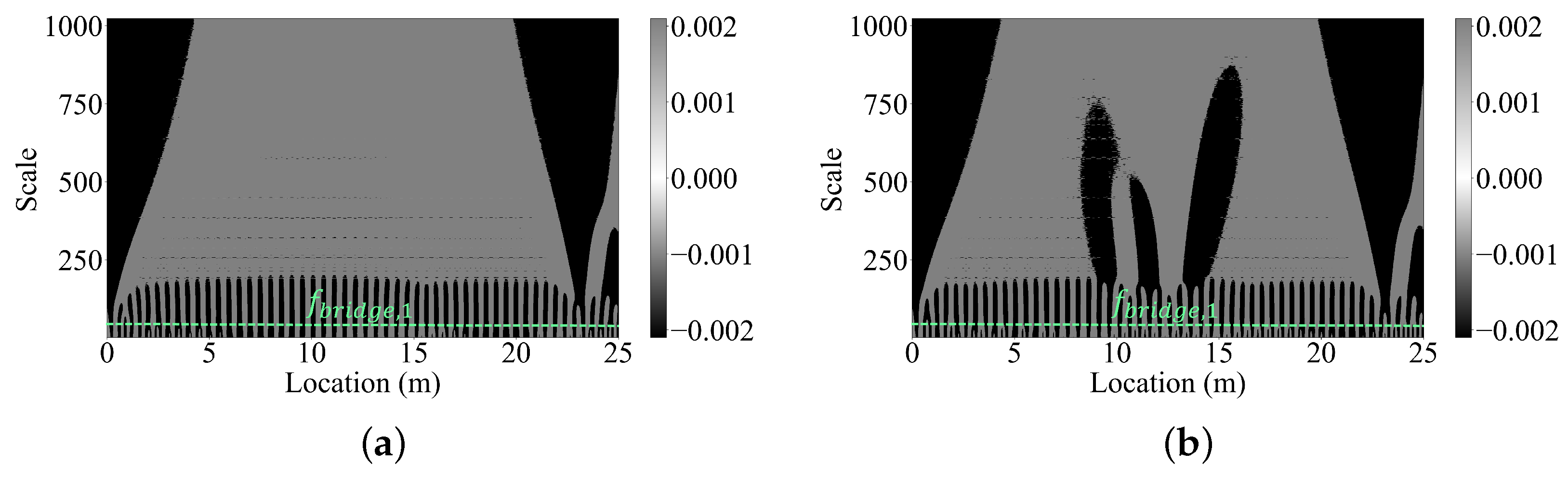
  • Determine the window which is sufficiently lower than the scale corresponding to the driving frequency and higher than the scales corresponding to the vehicle and the bridge frequencies. Decide on the scale where the horizontal section will be taken. Although, any scale within this window can be a viable option for the horizontal section, as they correspond to relatively low frequencies that capture static response, some engineering judgment can be required to select the final horizontal section.
  • Plot the horizontal section of the WCM at the selected scale for a bridge segment between x 0.2 L and x 0.8 L and evaluate the variation of the wavelet coefficients over the length of the bridge. Due to the edge effects that are commonly encountered in WCM of signals, the proposed method cannot detect damage that is located between 0–0.2 L and 0.8–1 L.
  • If the wavelet coefficients remain stable around zero, the bridge can be assessed to be undamaged. However, disturbances of the wavelet coefficients similar to those in Figure 9 indicate presence of damage.
  • Once damage is detected, its approximate location can be estimated as the point where the wavelet coefficients crosses the zero line between the negative and the positive peaks of the disturbance; see Figure 9.

4. Parametric Study

After demonstrating the efficacy of the proposed framework to detect and locate damage, we conducted a parametric study to evaluate the impact of different parameters on the damage estimates of the proposed framework. Accordingly, we repeated the numerical analysis by varying the following parameters: (1) Damage location and amount (2) vehicle speed (3) road roughness level (4) boundary conditions and (5) multiple damage.

4.1. Damage Location and Level
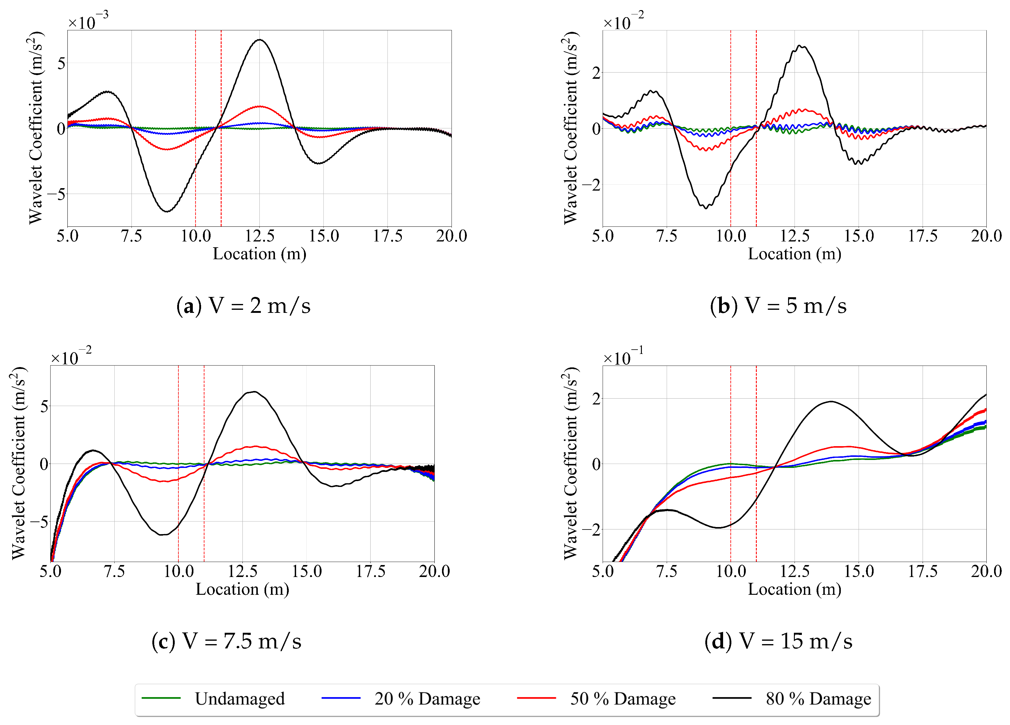
First, we will take a look at the efficacy of the proposed framework to detect and locate different levels of damage at different locations. For this, we simulated three different levels of damage that correspond to 20 % , 50 % , and 80 % reduction in the flexural stiffness of the bridge at three different segments. These segments start at 7 m, 12 m, and 16 m away from the left support of the bridge and are 1 m long. For each case, we first conducted a numerical analysis for a vehicle speed of 2 m/s and a sampling frequency of 1000 Hz. The road roughness profile in Figure 2 was considered in the analyses. We then carried out a continuous wavelet transform on the residual accelerations, which are computed by subtracting the accelerations recorded at the back-axle from those recorded at the front axle, to create the wavelet coefficient map for each case. Finally, we took a horizontal section of the wavelet coefficient maps at scale 600, which meets the criteria summarized above. Figure 11 presents the variation of the wavelet coefficients with location on the bridge for different damage locations and levels including the undamaged case. The plots are provided between x = 5 m and x = 20 m, i.e., 5 m away from each support due to the aforementioned edge effects.
In Figure 11, the damage location is marked by red-colored vertical dashed lines, and, for each damage location, the wavelet coefficients were plotted for the different damage levels. The wavelet coefficients for the undamaged case remain relatively stable at zero. On the other hand, induced damage creates a clear perturbation in the wavelet coefficient around the damage location, while they revert to zero once the vehicle travels away from the damage. As such, presence of damage can be successfully detected for each damage location and each damage level depicted in Figure 11. Further, the disturbances in the wavelet coefficients follow the unique pattern explained in Figure 11. Accordingly, the wavelet coefficients reach a negative peak before the damage location, start to increase crossing the horizontal axis close to the middle of the damaged segment on their path to a positive peak, which occurs after the damaged section. Hence, the location of the damage can successfully estimated for each damage location by the proposed method.
Further, the perturbations in the wavelet coefficient maps increase with an increase in the damage level paving the way for potentially quantifying the damage. However, this amplification in the perturbations with damage level, makes it difficult to visually identify the effect of 20 % damage on the wavelet coefficients when we plot all three damage levels in one plot. Therefore, we re-plotted the wavelet coefficients for the undamaged case and the 20 % damage between 12–13 m and 16–17 m cases in Figure 12. In this figure, we can clearly observe that, the wavelet coefficients for 20 % damage follows their counterparts for higher damage levels in Figure 11. Thus, we can confidently state that, the proposed framework can detect and locate damage for all damage levels and locations investigated.

4.2. Vehicle Speed

Next, we will take a look at the effect of vehicle speed on the accuracy of the proposed framework. The first immediate impact of the driving speed on the proposed framework is its effect on the driving frequency and the scale it corresponds to. As such, it is likely to alter the scale at which we take a horizontal section of the WCM. The shift in the scale corresponding to the driving frequency with the vehicle speed is demonstrated in the wavelet coefficient maps depicted in Figure 13 for different vehicle speeds. Recalling the procedure to select the scale where a horizontal section of the WCM will be taken, we first need to identify a range of scales which is sufficiently lower than the scale corresponding to the driving frequency and higher than the scales corresponding to the vehicle and the bridge frequencies. As shown in Figure 13 and also in Figure 10 for a speed of 2 m/s, which is not repeated here for brevity, this range is quite wide for lower vehicle speeds but gets narrower as the vehicle speed increases because the scale corresponding to the driving frequency decreases with increasing vehicle speed. Also depicted in the figure are the suitable ranges of scales for each vehicle speed to select the scale that will be used for damage detection and location. Accordingly, we selected the scales 600, 240, 240, and 185 for vehicle speeds of 2 m/s, 5 m/s, 7.5 m/s, and 15 m/s, respectively, as indicated by the dashed, red lines in Figure 13.
The variation of wavelet coefficients with the location of the vehicle on the bridge for different vehicle speeds at the respective scales are shown in Figure 14. The damage is located between x = 10 m and x = 11 m and the damage level varies between 20 % and 80 % . Figure 14 along with Figure 13 indicate that the accuracy of the proposed framework in detecting and locating damage decreases significantly with an increase in the vehicle speed.
This can be attributed to the fact that, the interaction between the driving frequency, bridge frequency and the vehicle frequency increases as the vehicle speed increases, i.e., when the driving frequency decreases. This interaction make it difficult to find a scale that is dominated by the static response, which is critical for the success of the proposed framework. Further, the dynamic response of the bridge is amplified significantly with an increase in the vehicle speed. As such, capturing the static response of the bridge becomes more difficult as the vehicle speed increases due to the increased dynamic response and the interaction between the driving, bridge and vehicle frequencies. Recalling that the proposed method owes its success in estimating the static displacements of the bridge, lower vehicle speeds lead to a much improved success rate in detecting and locating damage.

4.3. Road Roughness Level

As discussed above, road roughness is one of the parameters that adversely affect the success of drive-by monitoring methods in estimating bridge modal parameters and detecting damage. We also demonstrated in Section 3 that using residual accelerations, which are computed as the difference between the accelerations recorded on the front-axle and the rear-axle, eliminates these adverse effects. However, so far, we only tested the efficacy of this approach for one roughness level. This section investigates the effect of four distinct Class A roads on damage estimation of the bridge utilizing the proposed method. The roughness profiles were generated using Equations (1)–(3). The G ( n 0 ) value was specified as 0.01 × 10 6 m3, 0.1 × 10 6 m3, 1 × 10 6 m3, and 10 × 10 6 m3 for very low, low, moderate, and high roughness levels, respectively.
Figure 15 depicts the wavelet coefficients at a scale of 600 obtained from the residual accelerations for the different roughness levels. Different levels of damage is introduced between 10 m and 11 m. The speed of the vehicle was kept constant at 2 m/s. The results indicate that, despite the remedies taken to reduce its effect, road roughness still plays a significant role in detecting damage. For very low and low levels of road roughness, its effects are very limited and we can clearly detect the lowest levels of damage investigated in this study. However, once we reach the moderate roughness level, it becomes very difficult to distinguish the wavelet coefficients from the undamaged case and 20% damaged case. As such, only damage levels of 50% and above can be clearly identified for this roughness level. Finally, for the high roughness level, the fluctuations in the wavelet coefficients of the damaged case due to the road roughness become so significant that it is not possible to ascertain whether they are created by the damage or by the road roughness. Further for the moderate and high levels of road roughness, the wavelet coefficients for the undamaged bridge do not remain as stable as they do for the lower roughness levels, making it difficult for the proposed method to detect and locate the damage.
One question that needs to be considered here is: “If we do not know the road roughness level, how do we understand if the fluctuations are due to damage (e.g., Figure 15a) or due to road roughness (e.g., Figure 15d)”. This is a crucial question for the success of the practical applications of the proposed method. Focusing on Figure 15a,d, which depict the wavelet coefficients for very low and high roughness levels, respectively, we can observe that the fluctuations due to damage have mainly low frequency. On the other hand, fluctuations due to road roughness have significant high frequency components as can be observed from Figure 15d, and to a certain extent, Figure 15c. Therefore, the frequency content of the fluctuations in the wavelet coefficients should be examined to determine the source of the fluctuations in the wavelet coefficients to ascertain whether they are caused by road roughness or damage.

4.4. Boundary Conditions

To explore the impact of finite support stiffness on the efficacy of the proposed method, we substituted the pin-supports at both ends of the bridge with elastic springs. Commonly available bearings typically exhibit vertical stiffness ranging from k s p r = 1 × 10 5 kN/m and k s p r = 1 × 10 7 kN/m [63]. Hence, we systematically altered the vertical spring stiffness within this range, using equal values for the springs on both sides. Damage is introduced to the model as a 20 % , 50 % , and 80 % reduction in the bending stiffness of the bridge between x = 10 m and x = 11 m and the analyses were conducted for a vehicle speed of 2 m/s. Road profile A depicted in Figure 2 was used in the analysis.
Figure 16 presents the wavelet coefficients at a scale of 600 computed from the residual accelerations recorded on a vehicle crossing a bridge with different boundary conditions. Comparing Figure 16a,d, which represent the softest and stiffest boundary conditions, respectively, we can observe that the edge effects associated with the continuous wavelet transform are distributed over a longer section of the bridge when the softest bearing stiffness is used. As a result, the section of the bridge where damage can be identified using the proposed method becomes more limited. More specifically, for bearing stiffness of k s p r = 1 × 10 6 kN/m and higher, it is possible to detect damage between 5 m and 20 m away from the left support. On the other hand, for k s p r = 1 × 10 5 kN/m, the wavelet coefficients become flat only when the vehicle reaches 7.5 m due to the edge effects limiting the possible damage detection to a portion of the bridge between 7.5 m and 17.5 m. When the damage is simulated between 10m and 11m, as is the case in this study, the disturbance in the wavelet coefficients around the damage location can clearly be identified for all three levels of damage leading to successful detection and localization of damage.

4.5. Multiple Damage

Damage in bridges is not necessarily confined to one portion of the bridge, but, especially if created by environmental conditions, can occur simultaneously at different sections. To investigate the efficacy of the proposed method to detect damage at multiple locations, we simulated two scenarios where damage is introduced at two separate sections. In the first scenario, damage is simulated between 7 m and 8 m and also between 12 m and 13 m measured from the left-hand support. In the second scenario, the damage is between 7 m and 8 m and between 16 m and 17 m. In both scenarios, we focused only on 20% damage because detecting and locating this damage level ensures that higher damage levels can also be detected and located. The numerical analysis was then repeated for both scenarios with road roughness, and the residual accelerations on the vehicle were computed. The vehicle speed was 2 m/s. Figure 17 depicts the variation of the wavelet coefficients with location at a scale of 600.
Comparing Figure 12 and Figure 17, we can observe that multiple damage leads to two separate peaks (two each with positive and negative sign) with virtually the same amplitude in the wavelet coefficients when two separate sections of the bridge are damaged. On the other hand, only a one peak in the wavelet coefficients (one with negative and one with positive sign), that has a much higher amplitude, occurs when a single section of the bridge is damaged. Hence, presence of multiple damage can be detected using the proposed method in the form of multiple peaks in the wavelet coefficients.
Further, the peaks, and more specifically the location where the wavelet coefficient crosses the horizontal axis between the negative peak and the positive peak clearly indicates the location of the damage.
As such, we can confidently state that, for low vehicle speeds and relatively low road roughness levels, the proposed method can detect and locate multiple damage occurring concurrently on the bridge.

5. Concluding Remarks

This article summarizes a drive-by monitoring method that is based on the continuous wavelet transform of the residual accelerations recorded on a vehicle crossing the bridge. First, we demonstrated that, using the residual accelerations, which are computed by the accelerations recorded at the back axle from those recorded at the front axle, eliminates the adverse effects of road roughness on the wavelet coefficient maps. Once these effects are eliminated, the wavelet coefficients at a scale far away from the bridge, vehicle and driving frequencies, are shown to be stable around zero in the absence of damage. On the other hand, flexural damage leads to disturbances in the wavelet coefficients around the damage location. Leveraging this observation, the proposed method can detect and locate damage even in the absence of data from the undamaged bridge.
We also conducted a parametric study to investigate the effect of different parameters on the efficacy of the proposed method. Through this parametric study, we observed that:
  • The proposed method can successfully detect damage as low as 20 % at different locations of the bridge even in the presence of road roughness.
  • The proposed method illustrated that, as the damage level increases, perturbations in the wavelet coefficient maps also increase, potentially facilitating the quantification of damage. However, the proposed method cannot quantify the damage level in its current form when the damage is detected for the first time. However, as the damage propagates with time, repeated application of the proposed method enables the detection of the escalating damage levels.
  • The vehicle speed has a negative impact on damage detection using the proposed method because, as the vehicle speed increases the driving frequency becomes closer to the vehicle and bridge frequencies, minimizing the window that we select the scale used for damage detection. Hence, the proposed method should be used with low vehicle speeds to ensure successful damage detection.
  • Although using the residual accelerations largely eliminates the negative impacts of road roughness when road roughness is limited to low levels, for higher levels of road roughness, only higher levels of damage can be detected successfully.
  • Owing to the edge effects encountered in CWT, the proposed method is constrained to identifying and locating damage in regions where these edge effects are less pronounced.
  • When the bridge is seated on relatively soft bearings, the edge effects associated with continuous wavelet transform, is amplified and extends to a longer section of the bridge at the ends. As such, the segment of the bridge where damage can be detected becomes shorter. However, when the damage is close to the middle of the span and sufficiently away from the supports, the proposed method can successfully detect and locate damage.
  • The proposed method was also shown to detect and locate presence of multiple damaged sections. In the numerical analysis where we introduced damage in two separate sections of the bridge, we can clearly observe two peaks, both negative and positive, close to the damage locations, while we could only observe a single peak when only one bridge section was damaged. Further, as in the case of single damage, the wavelet coefficients reach a negative peak just before the damage location, increase after this peak, and cross the time axis at the middle of the bridge location before attaining a positive peak. Thus, using the proposed method, we can locate both damaged sections successfully.
One parameter that we did not include in the parametric study is the measurement noise. The main reason for omitting this parameter lies in the underlying principle of the proposed framework, which aims to capture the static response of the structure at low frequencies. Thus, the proposed framework is relatively immune to the effects of measurement noise, which is typically proportional to the square root of the bridge frequency, as indicated by most accelerometer manufacturers [49]. Additionally, Yang et al. [64] demonstrated that noise tends to affect bridge frequencies more prominently in the high frequency region, above 22 Hz, while having minimal impact on the first few frequencies. In this study, given that the damage component of the bridge was extracted from the wavelet scales corresponding to frequencies between 0.4 Hz and 1.0 Hz, that are situated far from the high frequency region where the measurement noise effects are most prominent. With that being said, the effects of measurement noise on the efficacy of the proposed framework should be investigated in future studies to confirm that the proposed framework is indeed immune to the adverse effects of this parameter.
Further, in future studies, the efficacy of the proposed method in detecting damage in three-dimensional structures should be investigated. Further, laboratory and field tests should be conducted to test its efficacy in physical applications. Finally, the method should be improved further to minimize the edge effects to ensure that damage close to the supports can also be successfully detected and located.

Author Contributions

Conceptualization, K.D. and E.E.; formal analysis, K.D; investigation, K.D.; writing—original draft preparation, K.D. and E.E.; methodology, K.D. and E.E.; supervision, E.E. All authors have read and agreed to the published version of the manuscript.

Funding

This research received no external funding.

Institutional Review Board Statement

Not applicable.

Informed Consent Statement

Not applicable.

Data Availability Statement

Data will be made available on request.

Conflicts of Interest

The authors declare no conflicts of interest.

References

  1. Corbally, R.; Malekjafarian, A. A data-driven approach for drive-by damage detection in bridges considering the influence of temperature change. Eng. Struct. 2022, 253, 113783. [Google Scholar] [CrossRef]
  2. Salehi, M.; Demirlioglu, K.; Erduran, E. Evaluation of the effect of operational modal analysis algorithms on identified modal parameters of railway bridges. In Proceedings of the IABSE Congress, Ghent—Structural Engineering for Future Societal Needs, Ghent, Belgium, 22–24 September 2021; pp. 22–24. [Google Scholar]
  3. Kamariotis, A.; Chatzi, E.; Straub, D. A framework for quantifying the value of vibration-based structural health monitoring. Mech. Syst. Signal Process. 2023, 184, 109708. [Google Scholar] [CrossRef]
  4. Gonen, S.; Demirlioglu, K.; Erduran, E. Optimal sensor placement for structural parameter identification of bridges with modeling uncertainties. Eng. Struct. 2023, 292, 116561. [Google Scholar] [CrossRef]
  5. Erduran, E.; Gonen, S.; Alkanany, A. Parametric analysis of the dynamic response of railway bridges due to vibrations induced by heavy-haul trains. Struct. Infrastruct. Eng. 2022, 20, 326–339. [Google Scholar] [CrossRef]
  6. Demirlioglu, K.; Gonen, S.; Erduran, E. On the Selection of Mode Shapes Used in Optimal Sensor Placement. In Sensors and Instrumentation, Aircraft/Aerospace and Dynamic Environments Testing, Volume 7: Proceedings of the 40th IMAC, A Conference and Exposition on Structural Dynamics 2022; Springer: Berlin/Heidelberg, Germany, 2022; pp. 85–92. [Google Scholar]
  7. Seo, J.; Hu, J.W.; Lee, J. Summary review of structural health monitoring applications for highway bridges. J. Perform. Constr. Facil. 2016, 30, 04015072. [Google Scholar] [CrossRef]
  8. Huffman, J.T.; Xiao, F.; Chen, G.; Hulsey, J.L. Detection of soil-abutment interaction by monitoring bridge response using vehicle excitation. J. Civ. Struct. Health Monit. 2015, 5, 389–395. [Google Scholar] [CrossRef]
  9. Gonen, S.; Demirlioglu, K.; Erduran, E. Modal Identification of a Railway Bridge Under Train Crossings: A Comparative Study. In Dynamics of Civil Structures, Volume 2: Proceedings of the 40th IMAC, A Conference and Exposition on Structural Dynamics 2022; Springer: Berlin/Heidelberg, Germany, 2022; pp. 33–40. [Google Scholar]
  10. Flammini, F.; Pragliola, C.; Smarra, G. Railway infrastructure monitoring by drones. In Proceedings of the 2016 International Conference on Electrical Systems for Aircraft, Railway, Ship Propulsion and Road Vehicles & International Transportation Electrification Conference (ESARS-ITEC), Toulouse, France, 2–4 November 2016; pp. 1–6. [Google Scholar]
  11. Kalaitzakis, M.; Kattil, S.R.; Vitzilaios, N.; Rizos, D.; Sutton, M. Dynamic structural health monitoring using a DIC-enabled drone. In Proceedings of the 2019 International Conference on Unmanned Aircraft Systems (ICUAS), Atlanta, GA, USA, 11–14 June 2019; pp. 321–327. [Google Scholar]
  12. Yang, Y.B.; Lin, C.; Yau, J. Extracting bridge frequencies from the dynamic response of a passing vehicle. J. Sound Vib. 2004, 272, 471–493. [Google Scholar] [CrossRef]
  13. Hajializadeh, D. Deep learning-based indirect bridge damage identification system. Struct. Health Monit. 2023, 22, 897–912. [Google Scholar] [CrossRef]
  14. Elhattab, A.; Uddin, N.; OBrien, E. Drive-by bridge frequency identification under operational roadway speeds employing frequency independent underdamped pinning stochastic resonance (FI-UPSR). Sensors 2018, 18, 4207. [Google Scholar] [CrossRef]
  15. He, Y.; Yang, J.P. Using acceleration residual spectrum from single two-axle vehicle at contact points to extract bridge frequencies. Eng. Struct. 2022, 266, 114538. [Google Scholar] [CrossRef]
  16. Erduran, E.; Pettersen, F.M.; Gonen, S.; Lau, A. Identification of Vibration Frequencies of Railway Bridges from Train-Mounted Sensors Using Wavelet Transformation. Sensors 2023, 23, 1191. [Google Scholar] [CrossRef]
  17. Li, Z.; Lin, W.; Zhang, Y. Bridge Frequency Scanning Using the Contact-Point Response of an Instrumented 3D Vehicle: Theory and Numerical Simulation. Struct. Control Health Monit. 2023, 2023. [Google Scholar] [CrossRef]
  18. Malekjafarian, A.; Khan, M.A.; OBrien, E.J.; Micu, E.A.; Bowe, C.; Ghiasi, R. Indirect monitoring of frequencies of a multiple span bridge using data collected from an instrumented train: A field case study. Sensors 2022, 22, 7468. [Google Scholar] [CrossRef]
  19. Sitton, J.D.; Rajan, D.; Story, B.A. Bridge frequency estimation strategies using smartphones. J. Civ. Struct. Health Monit. 2020, 10, 513–526. [Google Scholar] [CrossRef]
  20. Zhang, Y.; Wang, L.; Xiang, Z. Damage detection by mode shape squares extracted from a passing vehicle. J. Sound Vib. 2012, 331, 291–307. [Google Scholar] [CrossRef]
  21. Demirlioglu, K.; Gonen, S.; Erduran, E. Efficacy of vehicle scanning methods in estimating the mode shapes of bridges seated on elastic supports. Sensors 2023, 23, 6335. [Google Scholar] [CrossRef]
  22. Xu, H.; Liu, Y.; Yang, M.; Yang, D.; Yang, Y. Mode shape construction for bridges from contact responses of a two-axle test vehicle by wavelet transform. Mech. Syst. Signal Process. 2023, 195, 110304. [Google Scholar] [CrossRef]
  23. He, W.Y.; Ren, W.X.; Zuo, X.H. Mass-normalized mode shape identification method for bridge structures using parking vehicle-induced frequency change. Struct. Control Health Monit. 2018, 25, e2174. [Google Scholar] [CrossRef]
  24. Demirlioglu, K.; Gonen, S.; Erduran, E. Mode Shape Identification using Drive-by Monitoring: A comparative study. In Society for Experimental Mechanics Annual Conference and Exposition; Springer: Berlin/Heidelberg, Germany, 2023; pp. 57–66. [Google Scholar]
  25. González, A.; OBrien, E.J.; McGetrick, P. Identification of damping in a bridge using a moving instrumented vehicle. J. Sound Vib. 2012, 331, 4115–4131. [Google Scholar] [CrossRef]
  26. Yang, Y.; Zhang, B.; Chen, Y.; Qian, Y.; Wu, Y. Bridge damping identification by vehicle scanning method. Eng. Struct. 2019, 183, 637–645. [Google Scholar] [CrossRef]
  27. Shi, Z.; Uddin, N. Extracting multiple bridge frequencies from test vehicle–a theoretical study. J. Sound Vib. 2021, 490, 115735. [Google Scholar] [CrossRef]
  28. Keenahan, J.; Ren, Y.; OBrien, E.J. Determination of road profile using multiple passing vehicle measurements. Struct. Infrastruct. Eng. 2020, 16, 1262–1275. [Google Scholar] [CrossRef]
  29. Feng, K.; Casero, M.; González, A. Characterization of the road profile and the rotational stiffness of supports in a bridge based on axle accelerations of a crossing vehicle. Comput. Aided Civ. Infrastruct. Eng. 2023, 38, 1935–1954. [Google Scholar] [CrossRef]
  30. González, A.; Feng, K.; Casero, M. Detection, localisation and quantification of stiffness loss in a bridge using indirect drive-by measurements. Struct. Infrastruct. Eng. 2023, 2023, 1–19. [Google Scholar] [CrossRef]
  31. Lin, C.; Yang, Y. Use of a passing vehicle to scan the fundamental bridge frequencies: An experimental verification. Eng. Struct. 2005, 27, 1865–1878. [Google Scholar] [CrossRef]
  32. Kim, J.; Lynch, J.P. Experimental analysis of vehicle–bridge interaction using a wireless monitoring system and a two-stage system identification technique. Mech. Syst. Signal Process. 2012, 28, 3–19. [Google Scholar] [CrossRef]
  33. Siringoringo, D.M.; Fujino, Y. Estimating bridge fundamental frequency from vibration response of instrumented passing vehicle: Analytical and experimental study. Adv. Struct. Eng. 2012, 15, 417–433. [Google Scholar] [CrossRef]
  34. Yang, Y.; Xu, H.; Zhang, B.; Xiong, F.; Wang, Z. Measuring bridge frequencies by a test vehicle in non-moving and moving states. Eng. Struct. 2020, 203, 109859. [Google Scholar] [CrossRef]
  35. McGetrick, P.J.; Kim, C.W.; González, A.; Brien, E.J. Experimental validation of a drive-by stiffness identification method for bridge monitoring. Struct. Health Monit. 2015, 14, 317–331. [Google Scholar] [CrossRef]
  36. Xiao, F.; Sun, H.; Mao, Y.; Chen, G.S. Damage identification of large-scale space truss structures based on stiffness separation method. In Structures; Elsevier: Amsterdam, The Netherlands, 2023; Volume 53, pp. 109–118. [Google Scholar]
  37. OBrien, E.J.; Malekjafarian, A. A mode shape-based damage detection approach using laser measurement from a vehicle crossing a simply supported bridge. Struct. Control Health Monit. 2016, 23, 1273–1286. [Google Scholar] [CrossRef]
  38. Oshima, Y.; Yamamoto, K.; Sugiura, K. Damage assessment of a bridge based on mode shapes estimated by responses of passing vehicles. Smart Struct. Syst. 2014, 13, 731–753. [Google Scholar] [CrossRef]
  39. Zhang, Y.; Lie, S.T.; Xiang, Z. Damage detection method based on operating deflection shape curvature extracted from dynamic response of a passing vehicle. Mech. Syst. Signal Process. 2013, 35, 238–254. [Google Scholar] [CrossRef]
  40. Tan, C.; Zhao, H.; OBrien, E.J.; Uddin, N.; Fitzgerald, P.C.; McGetrick, P.J.; Kim, C.W. Extracting mode shapes from drive-by measurements to detect global and local damage in bridges. Struct. Infrastruct. Eng. 2021, 17, 1582–1596. [Google Scholar] [CrossRef]
  41. Tan, C.; Elhattab, A.; Uddin, N. “Drive-by’’ bridge frequency-based monitoring utilizing wavelet transform. J. Civ. Struct. Health Monit. 2017, 7, 615–625. [Google Scholar] [CrossRef]
  42. Mei, Q.; Gül, M.; Boay, M. Indirect health monitoring of bridges using Mel-frequency cepstral coefficients and principal component analysis. Mech. Syst. Signal Process. 2019, 119, 523–546. [Google Scholar] [CrossRef]
  43. Mei, Q.; Gül, M. A crowdsourcing-based methodology using smartphones for bridge health monitoring. Struct. Health Monit. 2019, 18, 1602–1619. [Google Scholar] [CrossRef]
  44. Mei, Q.; Gül, M.; Shirzad-Ghaleroudkhani, N. Towards smart cities: Crowdsensing-based monitoring of transportation infrastructure using in-traffic vehicles. J. Civ. Struct. Health Monit. 2020, 10, 653–665. [Google Scholar] [CrossRef]
  45. Sarwar, M.Z.; Cantero, D. Deep autoencoder architecture for bridge damage assessment using responses from several vehicles. Eng. Struct. 2021, 246, 113064. [Google Scholar] [CrossRef]
  46. Locke, W.; Sybrandt, J.; Redmond, L.; Safro, I.; Atamturktur, S. Using drive-by health monitoring to detect bridge damage considering environmental and operational effects. J. Sound Vib. 2020, 468, 115088. [Google Scholar] [CrossRef]
  47. Kildashti, K.; Alamdari, M.M.; Kim, C.; Gao, W.; Samali, B. Drive-by-bridge inspection for damage identification in a cable-stayed bridge: Numerical investigations. Eng. Struct. 2020, 223, 110891. [Google Scholar] [CrossRef]
  48. Zhang, B.; Qian, Y.; Wu, Y.; Yang, Y. An effective means for damage detection of bridges using the contact-point response of a moving test vehicle. J. Sound Vib. 2018, 419, 158–172. [Google Scholar] [CrossRef]
  49. Erduran, E.; Gonen, S. Contact point accelerations, instantaneous curvature, and physics-based damage detection and location using vehicle-mounted sensors. Eng. Struct. 2024, 304, 117608. [Google Scholar] [CrossRef]
  50. Hester, D.; González, A. A wavelet-based damage detection algorithm based on bridge acceleration response to a vehicle. Mech. Syst. Signal Process. 2012, 28, 145–166. [Google Scholar] [CrossRef]
  51. Hester, D.; González, A. A discussion on the merits and limitations of using drive-by monitoring to detect localised damage in a bridge. Mech. Syst. Signal Process. 2017, 90, 234–253. [Google Scholar] [CrossRef]
  52. Zhang, T.; Zhu, J.; Xiong, Z.; Zheng, K.; Wu, M. A new drive-by method for bridge damage inspection based on characteristic wavelet coefficient. Buildings 2023, 13, 397. [Google Scholar] [CrossRef]
  53. Salehi, M.; Erduran, E. Identification of boundary conditions of railway bridges using artificial neural networks. J. Civ. Struct. Health Monit. 2022, 12, 1223–1246. [Google Scholar] [CrossRef]
  54. Demirlioglu, K.; Gonen, S.; Erduran, E. Effect of Road Roughness on the Dynamic Response of Vehicles in Vehicle-Bridge Interaction Modeling. In International Conference on Experimental Vibration Analysis for Civil Engineering Structures; Springer Nature: Cham, Switzerland, 2023. [Google Scholar]
  55. Dodds, C.; Robson, J. The description of road surface roughness. J. Sound Vib. 1973, 31, 175–183. [Google Scholar] [CrossRef]
  56. ISO 8608; Road Surface Profiles–Reporting of Measured Data. International Standards Organisation: Geneva, Switzerland, 2016.
  57. Mallat, S. A Wavelet Tour of Signal Processing; Elsevier: Amsterdam, The Netherlands, 1999. [Google Scholar]
  58. Yang, Y.; Li, Y.; Chang, K. Effect of road surface roughness on the response of a moving vehicle for identification of bridge frequencies. Interact. Multiscale Mech. 2012, 5, 347–368. [Google Scholar] [CrossRef]
  59. González, A.; O’brien, E.J.; Li, Y.Y.; Cashell, K. The use of vehicle acceleration measurements to estimate road roughness. Veh. Syst. Dyn. 2008, 46, 483–499. [Google Scholar] [CrossRef]
  60. Harris, N.K.; González, A.; OBrien, E.J.; McGetrick, P. Characterisation of pavement profile heights using accelerometer readings and a combinatorial optimisation technique. J. Sound Vib. 2010, 329, 497–508. [Google Scholar] [CrossRef]
  61. Zhan, Y.; Au, F. Bridge surface roughness identification based on vehicle–bridge interaction. Int. J. Struct. Stab. Dyn. 2019, 19, 1950069. [Google Scholar] [CrossRef]
  62. Kong, X.; Cai, C.; Kong, B. Numerically extracting bridge modal properties from dynamic responses of moving vehicles. J. Eng. Mech. 2016, 142, 04016025. [Google Scholar] [CrossRef]
  63. Erduran, E.; Nordli, C.; Gonen, S. Effect of Elastomeric Bearing Stiffness on the Dynamic Response of Railway Bridges Considering Vehicle–Bridge Interaction. Appl. Sci. 2022, 12, 1952. [Google Scholar] [CrossRef]
  64. Yang, Y.; Xu, H.; Wang, Z.L.; Shi, K. Using vehicle–bridge contact spectra and residue to scan bridge’s modal properties with vehicle frequencies and road roughness eliminated. Struct. Control Health Monit. 2022, 29, e2968. [Google Scholar] [CrossRef]
Figure 1. Bridge and vehicle models.
Applsci 14 02969 g001
Figure 2. (a) The road roughness profile generated (b) Power Spectral Density of the road profile.
Applsci 14 02969 g002
Figure 3. (a) The displacement of the undamaged and damaged bridge under a moving vehicle (b) first mode shape of the undamaged and damaged bridges.
Applsci 14 02969 g003
Figure 4. Wavelet Coefficient Map of the rear-axle accelerations for smooth profile (a) Undamaged case (b) 50 % damage.
Applsci 14 02969 g004
Figure 5. Wavelet coefficients at scale 600 of the rear-axle accelerations for smooth profile and 50 % damage.
Applsci 14 02969 g005
Figure 6. Wavelet Coefficient Map of the rear-axle accelerations for rough profile (a) Undamaged case (b) 50 % damage.
Applsci 14 02969 g006
Figure 7. Wavelet coefficients at scale 600 of the rear-axle accelerations for rough profile and 50 % damage.
Applsci 14 02969 g007
Figure 8. Wavelet Coefficient Map of residual acceleration response for rough profile (a) undamaged case (b) 50 % damage.
Applsci 14 02969 g008
Figure 9. Wavelet coefficients at scale 600 for 50 % damage.
Applsci 14 02969 g009
Figure 10. Wavelet Coefficient Map between using vehicle’s residual acceleration response at 2 m/s for 50 % damage.
Applsci 14 02969 g010
Figure 11. Wavelet coefficients at scale 600 for different damage locations and amounts.
Applsci 14 02969 g011
Figure 12. Wavelet coefficients at scale 600 for 20 % damage at different locations for.
Applsci 14 02969 g012
Figure 13. Wavelet coefficient maps for different vehicle speeds.
Applsci 14 02969 g013
Figure 14. Wavelet coefficients at for different vehicle speeds.
Applsci 14 02969 g014
Figure 15. Wavelet coefficients at a scale of 600 for different roughness levels.
Applsci 14 02969 g015
Figure 16. Wavelet coefficients at a scale of 600 for different boundary conditions.
Applsci 14 02969 g016
Figure 17. Wavelet coefficients at scale 600 for 20 % damage at multiple locations. (a) Multiple damages between 7–8 m and between 12–13 m, (b) Multiple damages between 7–8 m and between 16–17 m.
Applsci 14 02969 g017
Table 1. The properties of bridge and instrumented vehicle [21].
BridgeMass per lengthρ = 2 t/m
Young’s modulus E = 30 GPa
Moment of inertiaI = 0.20 m4
First mode frequency f b , 1 = 4.35 Hz
Second mode frequency f b , 2 = 17.23 Hz
Third mode frequency f b , 3 = 38.06 Hz
VehicleMass m v = 5  t
Mass moment of Inertia J v = 3.5 t·m2
Stiffness coefficient (front) k 1 = 5750 kN/m
Stiffness coefficient (rear) k 2 = 2875 kN/m
Damping coefficient (front) c 1 = 2.5 kN·s/m
Damping coefficient (rear) c 2 = 2.5 kN·s/m
Axle distance to the mass d 1 = d 2 = 1 m
Bounce frequency f v , h = 5.77 Hz
Pitching frequency f v , r = 8.53 Hz
Disclaimer/Publisher’s Note: The statements, opinions and data contained in all publications are solely those of the individual author(s) and contributor(s) and not of MDPI and/or the editor(s). MDPI and/or the editor(s) disclaim responsibility for any injury to people or property resulting from any ideas, methods, instructions or products referred to in the content.

