A Boundary Scan Test Vectors Optimization Method Based on Improved GA-AO* Approach Considering Fault Probability Model

Abstract

The generation of test vectors is a key technique that affects the efficiency and fault detection rate of the boundary scan test. Aiming at the local optimal solution problem of the current common test vectors generation algorithm, this paper proposes a test vectors generation algorithm based on improved GA-AO* model, through which the test vectors are generated by using the idea of heuristic search and backtracking correction. In order to speed up the heuristic search, this paper designed a heuristic function with both prior and posterior parameters to describe the influence of typical faults on the failure probability index of the test vectors. At the same time, this paper used a genetic algorithm (GA) to determine the specific values of the posterior parameters iteratively. Finally, through theoretical analysis and physical verification, compared with the test vector generated by the traditional method, the test vector generated by this method is optimized on the prior failure probability index and performs better in the physical experiment.

1. Introduction

The boundary scan test is an advanced technique for digital circuit fault detection, which is widely used in large-scale digital circuit tests due to its fast and efficient testing advantages [1,2,3,4,5]. However, with the increase in IC density and complexity, the scale of boundary scan test vectors also increases rapidly, which leads to a decrease in test efficiency and fault detection precision [6,7]. How to generate a high-performance matrix of test vectors (MTV) for large-scale circuits has become a challenging problem [8,9,10].

In order to improve the quality of the MTV itself and achieve the goal of satisfying both test efficiency and fault isolation rate, many algorithms based on the mathematical characteristics of the test vector itself have been proposed, for example, counting sequence algorithm, modified counting sequence algorithm [11,12], Walking-1/0 sequence algorithm [13], W-test adaptive algorithm [14]. These methods are studied from the perspective of the mathematical characteristics of the MTV to achieve its optimization; they do not take into account the physical characteristics of the circuit under test. In order to bring the characteristics of the circuit itself and circuit fault into the scope of study, the limited fault model is proposed by researchers. Based on the physical distance between the networks in the circuit under test, the limited fault model calculates the prior probability of short-circuit fault and generates the MTV according to the probabilities, so that the MTV is further optimized. Ref. [15] uses the PSO algorithm to optimize the direction of generation for MTV; under the condition of maintaining the optimal test efficiency, the misjudgment rate and confusion rate of MTV are reduced. In Ref. [16], the genetic algorithm is used to optimize the grouping mode of circuit networks under test, and the MTV are optimized by assigning the networks with low probability of short circuit fault to the same test group. Ref. [17] describes the performance of MTV by fitness function and iterates test vectors with excellent performance by the genetic algorithm. Ref. [18] presents a method for optimizing test vectors based on fault information using the idea of heuristic. Ref. [19] provides a way to optimize test vectors by using randomly generated faults.

While keeping the testing efficiency unchanged, the above methods generate MTV by using intelligent iterative algorithm and reduce the misjudgment rate and confusion rate of MTV to some extent. However, the improper design of particle iteration and the difficulty to determine the search direction of these intelligent algorithms leads to the fast convergence in the optimization of misjudgment rate and confusion rate, the result is always trapped in the local optimal solution [20,21,22,23,24,25]. With the increase in the network size of the circuit under test, the local optimal solution of misjudgment rate and confusion rate will lead to a serious decline in the fault detection accuracy of the boundary scan [26,27,28]. A new approach to further optimize MTV is needed.

In this paper, an optimization method of MTV based on GA (Genetic Algorithm) and an improved AO*model is proposed. Firstly, this paper analyzes the mathematical model of interconnected short-circuit fault under the limited fault model and obtains the short-circuit fault mode which has the most influence on the circuit. After modeling the faults, this paper gives the evaluation indexes of misjudgment rate and confusion rate of MTV under these fault modes, and this paper sets the evaluation index of the MTVs to be optimized as the upper bound of the search and generates the MTV within the upper bound of the search by using the improved AO* model, which is an AND/OR graph search algorithm based on heuristic function and backtracking correction [29]; thus, the optimization of MTV is realized. To balance the search speed and the performance of the generated MTV, this paper sets the threshold and the number of threshold searches to improve the AO* model and adjusted the threshold in an adaptive way. At the same time, this paper establishes a heuristic function model combining the characteristics of the boundary scan test and the characteristics of the circuit under test and used a genetic algorithm to generate the parameters of the heuristic function that describe the characteristics of the circuit under test. When using the improved AO* model to generate MTV, this paper determines the generation direction according to the results of the heuristic function so that generation efficiency can be improved. This paper has the following innovations:

• A probability model of typical fault for the boundary scan test is established, and a new heuristic function is proposed based on this model to balance the test accuracy and the search efficiency of the algorithm.
• A method is designed to describe the characteristics of the system under test by using several undetermined parameters, which effectively improves the test precision of the complex circuit system.
• An improved AO* model with adaptive strategy is proposed to improve the MTV generation efficiency of complex circuit system.

This paper is organized as follows: In Section 2, this paper establishes and analyzes the mathematical model of interconnect short-circuit fault, then this paper identifies the most common types of faults. In Section 3, based on these fault characteristics, this paper gives the mathematical form of the heuristic function in AO* mode. Then, this paper uses the genetic algorithm to determine the parameters in the heuristic function, which are used to describe the characteristics of the actual circuit under test. After obtaining the heuristic function and the parameters, this paper uses the improved AO* model to generate the MTV. In Section 4, this paper uses different algorithms to generate MTV and compare them with the MTV generated by our method from the perspective of priori index and actual test results. Finally, the conclusion is wrapped up in Section 5.

2. Constructing the Probability Model of Typical Faults

During the manufacturing process of large-scale integrated circuit (LSI) systems, virtual soldering, de-soldering, and network short-circuit fault caused by soldering can easily occur. For an integrated circuit system with n networks, the probability of short-circuit fault between any two networks can be described by a symmetric matrix, as shown in Equation (1).

$$\begin{array}{cccc}0& p_{12}& \cdots & p_{1n}\\ p_{21}& 0& \cdots & p_{2n}\\ ⋮& ⋮& \ddots & ⋮\\ p_{n1}& p_{n2}& \cdots & 0\end{array}$$

(1)

The values of matrix elements $p_{ij}$ and $p_{ji}$ are equal, indicating the probability of a short-circuit fault occurring between the network numbered i and the network numbered j, and their values are calculated according to Equation (2).

$$p_{ij}=\left\{\begin{array}{c}{a}_0·A^{\left(1-\frac{L_{ij}}{L_0}\right)} L_0\le L_{ij}\le L_M\\ 0 otherwise\end{array}\right.$$

(2)

$a_0$ is the probability of a short-circuit between the nearest two networks, $L_0$ is the minimum distance between any two networks, $L_{ij}$ is the distance between net $N_i$ and net $N_j$, $L_M$ is the maximum physical distance between two nets capable of short-circuit failure, and A is an exponential decay function. The above parameters are determined according to the actual conditions of the integrated circuit system.

In this paper, it is called m-order short-circuit fault when the number of networks participating in the short-circuit fault is m. For a circuit with n networks $(m\le n)$, if each network is treated as a node of an undirected graph, and if a short-circuit fault occurs between networks, there is an edge between the corresponding nodes, the occurrence of an m-order short-circuit fault in this circuit is equivalent to the formation of a connected graph in which the number of nodes is according to the properties of connected graphs, and the minimum number of edges of m-nodes connected graphs is m − 1 [30,31]. Therefore, the number of possible m-order short-circuit faults is the number of connected graphs with m nodes and m − 1 edges, which equals the number of graphs with m nodes and m − 1 edges minus the number of all non-connected graphs with m nodes and m − 1 edges. Let the number of unconnected nodes in these graphs be t $(1\le t<m)$. According to the graph theory, the remaining m − t nodes can form $C_{m-t}^2$ edges at most. If the remaining m − t nodes form a graph with at least m − 1 edges, it must satisfy that $C_{m-t}^2\ge m-1$, so that t must satisfy the following conditions.

$$1\le t\le \frac{2m-1-\sqrt{8m-7}}{2}$$

(3)

If the largest integer value of t which satisfies Equation (3) is $t_0$, and this paper defines the number of graphs which have m − 1 edges and $m-t_0$ nodes as $K_0$, then $K_0$ can be calculated as follows:

$$K_0=C_{C_{m-t_0}^2}^{m-1}$$

(4)

Likewise, as this paper defines the number of graphs which have m − 1 edges and $m-t_0+1$ nodes as $K_1$, $K_1$ can be calculated as follows:

$$K_1=C_{C_{m-t_0+1}^2}^{m-1}-C_{m-t_0+1}^1·K_0$$

(5)

And similarly, as this paper defines the number of graphs which have m − 1 edges and $m$ nodes as $K_{t_0}$, $K_{t_0}$ can be calculated as follows:

$$K_{t_0}=C_{C_{m-t_0}^2}^{m-1}-\sum _{j=1}^{t_0}{C}_{m-t_0+j}^j ·K_{n-j}$$

(6)

The probabilities of these $K_{t_0}$ groups of m − 1 short-circuit faults in each group are taken out from Equation (1) and put into matrix $Q_m$, which is shown in Equation (7). Each line of $Q_m$ represents a combination of network short-circuit faults that can cause m-order short-circuit faults, and element $q_{ij}$ is the probability of these network short-circuit faults occurring.

$$\begin{array}{cccc}{q}_{11}& q_{12}& \cdots & q_{1(m-1)}\\ q_{21}& q_{22}& \cdots & q_{2(m-1)}\\ ⋮& ⋮& \ddots & ⋮\\ q_{K_{t_0}1}& q_{K_{t_0}2}& \cdots & q_{K_{t_0}(m-1)}\end{array}$$

(7)

Considering short-circuit faults between each network as independent events, the probability of m-order short-circuits faults ($P_m$) is as follows.

$$P_m=1-\prod _{i=1}^{K_{t_0}}\left(1-\prod _{j=1}^{m-1}{q}_{ij}\right)$$

(8)

Setting $P_{max}$ to the maximum of short-circuit faults probability $q_{ij}$, we obtain the following relationship:

$$P_m\le 1-(1-{P_{max}}^{m-1}{)}^{K_{t_0}}$$

(9)

Setting $P_{Mm}$ to the upper bound of m-order short-circuit faults probability $P_m$, its value is as follows.

$$P_{Mm}=1-(1-{P_{max}}^{m-1}{)}^{K_{t_0}}$$

(10)

$P_{max}$ is a value far less than 1. With 0.001 as the step size of $P_{max}$ change, $P_{Mm}$ varies with m, as shown in Figure 1.

Equations (4)–(10) are the probability models of typical faults established in this paper. By this probability model, the upper bounds of the probability of short-circuit faults of each order can be calculated. According to the calculation results, this paper analyzes and studies those fault modes with high probability, so as to improve the efficiency of the following algorithms while ensuring the test precision.

As shown in Figure 1, the probability of a fault with order greater than 3 approaches 0, so the short-circuit fault model established in this paper only considers short-circuit faults with order no greater than 3.

3. Proposed Method

3.1. Method Overview

The heuristic function is the key of using the GA-AO* approach to generate MTV. If the calculation of heuristic function is much bigger than the true value, the result of AO* will have a bad performance. On the contrary, if the calculation of heuristic function is much smaller than true value, the efficiency of AO* will become too low to solve such an NP-hard question. In order to have an appropriate heuristic function, firstly, this paper established the model of evaluation index—${\mathrm{P}}_{\mathrm{M}\mathrm{T}\mathrm{V}}$. Based on the characteristics of ${\mathrm{P}}_{\mathrm{M}\mathrm{T}\mathrm{V}}$, this paper determined the mathematical form of heuristic function and used both prior and posterior parameters to describe the question. Among them, the prior parameters were obtained by calculation, and the posterior parameters were obtained by the genetic algorithm (GA) based on the characteristics of the system under test. After obtaining the heuristic function, this paper judges whether the relative error of estimated value of ${\mathrm{P}}_{\mathrm{M}\mathrm{T}\mathrm{V}}$ calculated by the heuristic function is lower than the condition proposed by testers. If it meets the condition, this paper uses it to choose the search direction for the AO* and uses the AO* to generate the MTV. In addition, in order to improve the efficiency of the AO* algorithm, the adaptive strategy is used to improve it. The above process is shown in Figure 2.

3.2. Failure Probability of the Matrix of Test Vectors

The process of interconnect test of the integrated circuit system by boundary scan technique is injecting MTV (matrix of test vectors) and reading MRV (matrix of response vectors), by comparing the difference between them to carry out the fault diagnosis process. A schematic of the structure of the boundary scan test is shown in Figure 3. This architecture is proposed by IEEE1149.1 standard, which is based on JTAG (Joint Test Action Group) interface and BSC (Boundary Scan Cell) [32]. The TDI and TDO ports of the JTAG interface of the chip under test are connected in the form of daisy chain. During each test, the test vectors move into the boundary scan test unit through the TDI serial of each chip, motivating the corresponding pins. After the excitation, the response vectors are displaced from the TDO port of the chip. The whole testing process is controlled by TCK and TMS signals in the form of a bus.

The elements of MTV are logical values of 0 or 1. The rows of the matrix which are called STV (Sequential Test Vector) represent the logical values that are applied to the same network in multiple boundary scan test cycles. The columns of the matrix which are called PTV (Parallel Test Vector) represent vectors composed of logical values that are loaded onto each network during a boundary scan test cycle. MTV is as follows.

$$\begin{array}{cccc}{a}_{11}& a_{12}& \cdots & a_{1m}\\ a_{21}& a_{22}& \cdots & a_{2m}\\ ⋮& ⋮& \ddots & ⋮\\ a_{n1}& a_{n2}& \cdots & a_{nm}\end{array}$$

(11)

The number of MTV’s rows(n) is equal to the number of networks under test. The number of MTV’s rows(m) is called compactness index, which needs to satisfy the following requirements.

$$m\ge {log}_2(n+2)$$

(12)

The rows of MRV are called SRV (Sequential Response Vector). Each SRV is a collection of logical values received on a network in the circuit under test. The columns of MRV are called PRV (Parallel Response Vector). Each SRV is a collection of logical values received from a network in one cycle of the boundary scan test. When short-circuit faults occur between networks, the SRVs received from the fault networks are presented as a result of wired-AND of STVs (wired-AND and wired-OR are dual models. There is only one situation in the same circuit, so this paper only discusses wired-AND here). By observing which networks SRV is the result of corresponding STVs wired-AND, testers can judge which networks have a short-circuit fault.

On this basis, the definition of the short-circuit fault diagnosis through the SRV network with the phenomenon of misjudgment and confusion is as follows.

Misjudgment: When an STV injected into one network is the same as the result of wired-AND of STVs injected into another group of networks. It is not possible to judge whether there is a short-circuit failure between this network and this set of networks. At this point, a misjudgment has occurred on the MTV. As an example, shown in Figure 4, the result of wired-AND of the STV injected into net1 and net2 is the same as the STV injected into net3, when a short-circuit fault occurs between net1 and net2, testers cannot determine whether net3 has a short-circuit fault with them (as shown by the red dotted line), so the misjudgment occurred.

Confusion: When the result of wired-AND of a group STVs is the same as the result of wired-AND of another group STVs (There is no overlap between them). It is not possible to judge whether there is a short-circuit failure between these two groups of networks. At this point, a confusion has occurred on the MTV. As an example, shown in Figure 5, the result of wired-AND of the STV injected into net1, net2, and net4 is the same as the result of wired-AND of STV injected into net3 and net5, when a short-circuit fault occurs between net1, net2, and net4, and a short-circuit fault occurs between net3 and net5. Testers cannot determine whether the first group of nets have a short-circuit fault with the second (as shown by the red dotted line), so the confusion occurred.

Based on the analysis in Section 3.1 of this paper, the fault model considered in this paper is 2-order, 3-order short-circuit fault model. At the same time, it is stipulated that the test vectors generated in this paper are all carried out under the optimal compactness index, that is, the number of columns(m) of MTV is an upward rounding of ${log}_2(n+2)$.

Under this premise, we can divide the phenomenon of misjudgment and confusion in MTV into the following kinds of events:

• Misjudgment caused by 2-order short-circuit: the result of wired-AND of 2 STVs is the same as another STV.
• Misjudgment caused by 3-order short-circuit: the result of wired-AND of 3 STVs is the same as another STV.
• Confusion caused by 2-order short-circuit: the result of wired-AND of 2 STVs is the same as the result of wired-AND of other 2 STVs.

Definition: The failure probability of MTV ($P_{MTV}$) is the probability of the above three events in a set of STVs. Let S be the set of STVs. Let power set $A\in 2^S$, and $\left|A\right|=2$. Let power set $B\in 2^S$, and |B| = 3. Let power set $C\in 2^A$, and |C| = 2, it can be calculated by the following equation.

$$\begin{array}{c}{P}_{MTV}=1-\prod _{\left[{STV}_{i1},{STV}_{i2}\right]\in A}(1-k_{i1i2}·p_{i1i2})·\prod _{\left[{STV}_{i1},{STV}_{i2},{STV}_{i3}\right]\in B}(1-k_{i1i2i3}·p_{i1i2i3})\\ ·\prod _{\left[{(STV}_{i1},{STV}_{i2}),{(STV}_{i3},{STV}_{i4})\right]\in C}(1-k_{i1i2i3i4}·p_{i1i2}·p_{i3i4})\end{array}$$

(13)

$p_{i1i2}$ is the probability of 2-order short-circuiting fault between networks i1 and i2. $p_{i1i2i3}$ is the probability of 3-order short-circuit fault between networks i1, i2, and i3. When the 2-order short-circuit between i1 and i2 causes misjudgment, $k_{i1i2}$ is 1, otherwise it is 0. When the 3-order short-circuit between i1, i2, i3 causes misjudgment, $k_{i1i2i3}$ is 1, otherwise it is 0. When the 2-order short-circuit between i1 and i2 and 2-order short-circuit between i3 and i4 causes confusion, $k_{i1i2i3i4}$ is 1, otherwise it is 0.

Since different networks have different short-circuit probabilities, and each network corresponds to an STV in MTV, and if each STV in MTV is treated as a unit of a sequence, the whole MTV is treated as a sequence, then the generation of MTV problem with minimum $P_{MTV}$ will transform into the optimal cost sequence search problem.

3.3. Heuristic Function Based on the Characteristics of MTV

The generation of MTV using AO* model includes forward searching and backward tracing. In the forward searching, let the test vector matrix composed of STVs from the first row to row $i$ be a sub-matrix ${MTV}_i$, as shown in Equation (14).

$${MTV}_n\left\{\begin{array}{c}\begin{array}{c}{MTV}_i\left\{\begin{array}{c}{MTV}_2\left\{\begin{array}{c}{MTV}_1\{\\ \begin{array}{c}\end{array}\end{array}\right.\\ \begin{array}{c}\end{array}\\ \begin{array}{c}\end{array}\end{array}\right.\\ \\ \end{array}\end{array}\begin{array}{cccc}{a}_{11}& a_{12}& \cdots & a_{1m}\\ a_{21}& a_{22}& \cdots & a_{2m}\\ ⋮& ⋮& \ddots & ⋮\\ a_{i1}& a_{i2}& \cdots & a_{im}\\ ⋮& ⋮& \ddots & ⋮\\ a_{n1}& a_{n2}& \cdots & a_{nm}\end{array}\right.$$

(14)

The heuristic function $f\left({MTV}_i\right)$ will calculate the ${\widehat{P}}_{{MTV}_i}$ (estimated $P_{MTV}$) of the sub-matrix ${MTV}_i$, then this paper will choose the ${MTV}_i$ with least ${\widehat{P}}_{{MTV}_i}$ as a direction of searching. ${\widehat{P}}_{{MTV}_i}$ is calculated by Equation (15).

It represents an estimate of the $P_{MTV}$ of the MTV after completing the remaining n−i rows if the previous i-row STVs are ${MTV}_i$.

$${\widehat{P}}_{{MTV}_i}=P_{{MTV}_i}+f\left({MTV}_i\right)-P_{{MTV}_i}·f\left({MTV}_i\right)$$

(15)

The implication of the $f\left({MTV}_i\right)$ is to estimate the $P_{MTV}$ of the MTV after generation based on the information of STVs in former i row, that is, to evaluate the impact of the STVs in former i row in the future. According to the analysis of Section 3.2, for a given STV, its effect on $P_{MTV}$ can be divided into three types of events:

• The result of wired-AND between it and other STVs is the same as other STVs in latter n−i rows, thus leading to misjudgment.
• The result of wired-AND of other STVs (at least one of those STVs is from latter n−i row) is the same as it, thus leading to misjudgment.
• The result of wired-AND between it and another STV is the same as the result of wired-AND of another two STVs (at least one of those three STVs is from latter n−i row), thus leading to confusion.

These events can be divided into 13 cases, depending on whether STVs belong to the former i row or latter n−i row, and the order of wired-AND. For a given STV, each case is independent. Let $f_{jk}$ be the estimate of influence on $P_{MTV}$ of the case k ($1\le k\le 13$) of ${STV}_j$ (the row j of ${MTV}_i$). Then, $f\left({MTV}_i\right)$ can be represented by the following Equation (16).

$$f\left({MTV}_i\right)=\prod _{j=1}^i\prod _{k=1}^{13}{f}_{jk}$$

(16)

According to the analysis of the 3.2, the effect of each case on $P_{MTV}$ is represented by $P_{MTV}$ times $(1-P_k)$. Under the premise of randomly assigning STV, $P_k$ is the probability that case k will occur according to the classical probability. At the same time, for a given ${STV}_j$, there are different random combinations that make the case k occur, and the occurrence of these combinations is independent of each other, If the number of these combinations is $D_{jk}$, then the effect of $P_{MTV}$ is the product of all the results, which is $(1-P_k{)}^{D_{jk}}$. Considering the characteristics of the different circuits, it is necessary to add parameters $\beta$ to describe the characteristics of the circuits in each case, so the final form of $f_{jk}$ is as follows:

$$f_{jk}=(1-{\beta }_k·P_{jk}{)}^{D_{jk}}$$

(17)

For a $n\times m$ MTV and each of its sub-matrix ${MTV}_i$, set $N_a=2^m-2$, $N_a$ denotes the number of all types of STV with length m, that is, the number of 0/1 sequences with length m. Set $N_s=2^m-2-i$, $N_s$ denotes the number of available STV types left when the former i rows have been set. Set $N_e=n-i$, $N_e$ denotes the number of STVs waiting to be set. $N_{j1}$ is the number of 1 in ${STV}_j$, $N_{j0}$ is the number of 0 in ${STV}_j$, the calculation and range of $P_{jk}$ and $D_{jk}$ in Equation (17) are shown in

Table 1. The calculation and range of $P_{jk}$ and $D_{jk}$.

k	${\mathit{D}}_{\mathit{j}\mathit{k}}$	${\mathit{P}}_{\mathit{j}\mathit{k}}$	Range
1	$\frac{{\mathrm{C}}_{{\mathrm{N}}_{\mathrm{a}}-2}^{{\mathrm{N}}_{\mathrm{s}}-2}}{{\mathrm{C}}_{{\mathrm{N}}_{\mathrm{a}}}^{{\mathrm{N}}_{\mathrm{s}}}}·\frac{{\mathrm{C}}_{{\mathrm{N}}_{\mathrm{s}}-2}^{{\mathrm{N}}_{\mathrm{e}}-2}}{{\mathrm{C}}_{{\mathrm{N}}_{\mathrm{s}}}^{{\mathrm{N}}_{\mathrm{e}}}}$	${\displaystyle \sum _{\mathrm{t}=1}^{\frac{{\mathrm{N}}_{\mathrm{j}1}}{2}}}{\mathrm{C}}_{{\mathrm{N}}_{\mathrm{j}1}}^{\mathrm{t}}$	$N_{j1}\ge 3$
2	$\frac{{\mathrm{C}}_{{\mathrm{N}}_{\mathrm{a}}-3}^{{\mathrm{N}}_{\mathrm{s}}-3}}{{\mathrm{C}}_{{\mathrm{N}}_{\mathrm{a}}}^{{\mathrm{N}}_{\mathrm{s}}}}·\frac{{\mathrm{C}}_{{\mathrm{N}}_{\mathrm{s}}-3}^{{\mathrm{N}}_{\mathrm{e}}-3}}{{\mathrm{C}}_{{\mathrm{N}}_{\mathrm{s}}}^{{\mathrm{N}}_{\mathrm{e}}}}$	${\displaystyle \sum _{\mathrm{t}=1}^{\frac{{\mathrm{N}}_{\mathrm{j}1}}{3}}}{\displaystyle \sum _{\mathrm{u}=1}^{\frac{{\mathrm{N}}_{\mathrm{j}1}-\mathrm{t}}{2}}}{\mathrm{C}}_{{\mathrm{N}}_{\mathrm{j}1}}^{\mathrm{t}}·{\mathrm{C}}_{{\mathrm{N}}_{\mathrm{j}1}-\mathrm{t}}^{\mathrm{u}}$	$N_{j1}\ge 4$
3	$\frac{{\mathrm{C}}_{{\mathrm{N}}_{\mathrm{a}}-2}^{{\mathrm{N}}_{\mathrm{s}}-2}}{{\mathrm{C}}_{{\mathrm{N}}_{\mathrm{a}}}^{{\mathrm{N}}_{\mathrm{s}}}}·\frac{{\mathrm{C}}_{{\mathrm{N}}_{\mathrm{s}}-2}^{{\mathrm{N}}_{\mathrm{e}}-2}}{{\mathrm{C}}_{{\mathrm{N}}_{\mathrm{s}}}^{{\mathrm{N}}_{\mathrm{e}}}}$	${\displaystyle \sum _{\mathrm{t}=1}^{{\mathrm{N}}_{\mathrm{j}0}-1}}{\mathrm{C}}_{\mathrm{n}}^{\mathrm{t}}$	$N_{j0}\ge 3$
4	$\frac{{\mathrm{C}}_{{\mathrm{N}}_{\mathrm{a}}-3}^{{\mathrm{N}}_{\mathrm{s}}-3}}{{\mathrm{C}}_{{\mathrm{N}}_{\mathrm{a}}}^{{\mathrm{N}}_{\mathrm{s}}}}·\frac{{\mathrm{C}}_{{\mathrm{N}}_{\mathrm{s}}-3}^{{\mathrm{N}}_{\mathrm{e}}-3}}{{\mathrm{C}}_{{\mathrm{N}}_{\mathrm{s}}}^{{\mathrm{N}}_{\mathrm{e}}}}$	${\displaystyle \sum _{\mathrm{t}=2}^{{\mathrm{N}}_{\mathrm{j}0}-1}}{\displaystyle \sum _{\mathrm{u}=1}^{\frac{\mathrm{t}}{2}}}{\mathrm{C}}_n^{\mathrm{t}}·{\mathrm{C}}_{\mathrm{t}}^{\mathrm{u}}$	$N_{j0}\ge 4$
5	$\frac{{\mathrm{C}}_{{\mathrm{N}}_{\mathrm{a}}-4}^{{\mathrm{N}}_{\mathrm{s}}-4}}{{\mathrm{C}}_{{\mathrm{N}}_{\mathrm{a}}}^{{\mathrm{N}}_{\mathrm{s}}}}·\frac{{\mathrm{C}}_{{\mathrm{N}}_{\mathrm{s}}-4}^{{\mathrm{N}}_{\mathrm{e}}-4}}{{\mathrm{C}}_{{\mathrm{N}}_{\mathrm{s}}}^{{\mathrm{N}}_{\mathrm{e}}}}$	${\displaystyle \sum _{\mathrm{t}=2}^{{\mathrm{N}}_{\mathrm{j}1}-1}}{\displaystyle \sum _{\mathrm{u}=1}^{\frac{\mathrm{t}+{\mathrm{N}}_{\mathrm{j}1}}{2}}}({\mathrm{C}}_{{\mathrm{N}}_{\mathrm{j}0}}^{\mathrm{t}}·{\mathrm{C}}_{\mathrm{t}+{\mathrm{N}}_{\mathrm{j}1}}^{\mathrm{u}}-1)$	$N_{j1}\ge 1$
6	$\frac{{\mathrm{C}}_{{\mathrm{N}}_{\mathrm{a}}-1}^{{\mathrm{N}}_{\mathrm{s}}-1}}{{\mathrm{C}}_{{\mathrm{N}}_{\mathrm{a}}}^{{\mathrm{N}}_{\mathrm{s}}}}·\frac{{\mathrm{C}}_{{\mathrm{N}}_{\mathrm{s}}-1}^{{\mathrm{N}}_{\mathrm{e}}-1}}{{\mathrm{C}}_{{\mathrm{N}}_{\mathrm{s}}}^{{\mathrm{N}}_{\mathrm{e}}}}$	$1$	$N_{j1}<n$
7	$\frac{{\mathrm{C}}_{{\mathrm{N}}_{\mathrm{a}}-2}^{{\mathrm{N}}_{\mathrm{s}}-2}}{{\mathrm{C}}_{{\mathrm{N}}_{\mathrm{a}}}^{{\mathrm{N}}_{\mathrm{s}}}}·\frac{{\mathrm{C}}_{{\mathrm{N}}_{\mathrm{s}}-2}^{{\mathrm{N}}_{\mathrm{e}}-2}}{{\mathrm{C}}_{{\mathrm{N}}_{\mathrm{s}}}^{{\mathrm{N}}_{\mathrm{e}}}}$	${\displaystyle \sum _{\mathrm{t}=1}^{\frac{{\mathrm{N}}_{\mathrm{j}1}}{2}}}{\mathrm{C}}_{{\mathrm{N}}_{\mathrm{j}1}}^{\mathrm{t}}-1$	$N_{j1}\ge 3$
8	$\frac{{\mathrm{C}}_{{\mathrm{N}}_{\mathrm{a}}-2}^{{\mathrm{N}}_{\mathrm{s}}-2}}{{\mathrm{C}}_{{\mathrm{N}}_{\mathrm{a}}}^{{\mathrm{N}}_{\mathrm{s}}}}·\frac{{\mathrm{C}}_{{\mathrm{N}}_{\mathrm{s}}-2}^{{\mathrm{N}}_{\mathrm{e}}-2}}{{\mathrm{C}}_{{\mathrm{N}}_{\mathrm{s}}}^{{\mathrm{N}}_{\mathrm{e}}}}$	${\displaystyle \sum _{\mathrm{t}=1}^{{\mathrm{N}}_{\mathrm{j}0}-1}}{\mathrm{C}}_{{\mathrm{N}}_{\mathrm{j}0}}^{\mathrm{t}}$	$N_{j0}\ge 2$
9	$\frac{{\mathrm{C}}_{{\mathrm{N}}_{\mathrm{a}}-1}^{{\mathrm{N}}_{\mathrm{s}}-1}}{{\mathrm{C}}_{{\mathrm{N}}_{\mathrm{a}}}^{{\mathrm{N}}_{\mathrm{s}}}}·\frac{{\mathrm{C}}_{{\mathrm{N}}_{\mathrm{s}}-1}^{{\mathrm{N}}_{\mathrm{e}}-1}}{{\mathrm{C}}_{{\mathrm{N}}_{\mathrm{s}}}^{{\mathrm{N}}_{\mathrm{e}}}}$	$1$	$N_{j0}\ge 1$
10	$\frac{{\mathrm{C}}_{{\mathrm{N}}_{\mathrm{a}}-2}^{{\mathrm{N}}_{\mathrm{s}}-2}}{{\mathrm{C}}_{{\mathrm{N}}_{\mathrm{a}}}^{{\mathrm{N}}_{\mathrm{s}}}}·\frac{{\mathrm{C}}_{{\mathrm{N}}_{\mathrm{s}}-2}^{{\mathrm{N}}_{\mathrm{e}}-2}}{{\mathrm{C}}_{{\mathrm{N}}_{\mathrm{s}}}^{{\mathrm{N}}_{\mathrm{e}}}}$	${\displaystyle \sum _{\mathrm{t}=1}^{\frac{{\mathrm{N}}_{\mathrm{j}0}}{2}}}{\mathrm{C}}_{{\mathrm{N}}_{\mathrm{j}0}}^{\mathrm{t}}-1$	$N_{j0}\ge 3$
11	$\frac{{\mathrm{C}}_{{\mathrm{N}}_{\mathrm{a}}-3}^{{\mathrm{N}}_{\mathrm{s}}-3}}{{\mathrm{C}}_{{\mathrm{N}}_{\mathrm{a}}}^{{\mathrm{N}}_{\mathrm{s}}}}·\frac{{\mathrm{C}}_{{\mathrm{N}}_{\mathrm{s}}-3}^{{\mathrm{N}}_{\mathrm{e}}-3}}{{\mathrm{C}}_{{\mathrm{N}}_{\mathrm{s}}}^{{\mathrm{N}}_{\mathrm{e}}}}$	${\displaystyle \sum _{\mathrm{t}=2}^{{\mathrm{N}}_{\mathrm{j}0}-1}}{\displaystyle \sum _{\mathrm{u}=1}^{\frac{\mathrm{t}}{2}}}{\mathrm{C}}_n^{\mathrm{t}}·{\mathrm{C}}_{\mathrm{t}}^{\mathrm{u}}$	$N_{j0}\ge 4$
12	$\frac{{\mathrm{C}}_{{\mathrm{N}}_{\mathrm{a}}-4}^{{\mathrm{N}}_{\mathrm{s}}-4}}{{\mathrm{C}}_{{\mathrm{N}}_{\mathrm{a}}}^{{\mathrm{N}}_{\mathrm{s}}}}·\frac{{\mathrm{C}}_{{\mathrm{N}}_{\mathrm{s}}-4}^{{\mathrm{N}}_{\mathrm{e}}-4}}{{\mathrm{C}}_{{\mathrm{N}}_{\mathrm{s}}}^{{\mathrm{N}}_{\mathrm{e}}}}$	${\displaystyle \sum _{\mathrm{t}=2}^{{\mathrm{N}}_{\mathrm{j}0}-1}}{\displaystyle \sum _{\mathrm{u}=1}^{\frac{\mathrm{t}+{\mathrm{N}}_{\mathrm{j}0}}{2}}}({\mathrm{C}}_{{\mathrm{N}}_{\mathrm{j}1}}^{\mathrm{t}}·{\mathrm{C}}_{\mathrm{t}+{\mathrm{N}}_{\mathrm{j}0}}^{\mathrm{u}}-1)$	$N_{j0}\ge 1$
13	$\frac{{\mathrm{C}}_{{\mathrm{N}}_{\mathrm{a}}-1}^{{\mathrm{N}}_{\mathrm{s}}-1}}{{\mathrm{C}}_{{\mathrm{N}}_{\mathrm{a}}}^{{\mathrm{N}}_{\mathrm{s}}}}·\frac{{\mathrm{C}}_{{\mathrm{N}}_{\mathrm{s}}-1}^{{\mathrm{N}}_{\mathrm{e}}-1}}{{\mathrm{C}}_{{\mathrm{N}}_{\mathrm{s}}}^{{\mathrm{N}}_{\mathrm{e}}}}$	$1$	$N_{j0}<n$

. For a sub-matrix ${MTV}_i$, firstly, this paper calculates its $N_a$, $N_s$, and $N_e$ according to i. Then, this paper counts the number of 1 and 0 in each row of ${MTV}_i$ from the row 1 to the row i to obtain $N_{j1}$ and $N_{j0}$. Using the parameters above, $P_{jk}$ and $D_{jk}$ can be calculated from Table 1. When out of the range shown in the table below, $f_{jk}$ = 1, indicating that case k cannot occur at this time and has no effect on $P_{MTV}$.

3.4. Parameter Determination Method of Heuristic Function Based on Improved Genetic Algorithm

After the analysis of Section 3.3, this paper establishes the heuristic function with 13 parameters. These parameters are used to describe the characteristics of the circuit under 13 different fault cases. In this section, this paper will use the improved genetic algorithm to determine the value of these parameters. For circuits under test with network number of n, this paper randomly generates a large number of MTVs. For each MTV, this paper calculates the ${\widehat{P}}_{{MTV}_i}$ for each of its sub-matrices ${MTV}_i$ $(1\le i\le n)$ in turn, and averages the ${\widehat{P}}_{{MTV}_i}$ of all the ${MTV}_i$, so that this paper can obtain a function $F\left(i\right)$ which is only related to i. According to Equation (17), ${\widehat{P}}_{\mathrm{M}\mathrm{T}\mathrm{V}}$ contains 13 undetermined parameters $\beta$; these parameters can be determined by fitting $F\left(i\right)$, for $F\left(i\right)$ includes the $P_{{MTV}_i}$ of the sub-matrix ${MTV}_i$ itself and the estimated impact on $P_{\mathrm{M}\mathrm{T}\mathrm{V}}$. For each MTV, this paper will calculate its $P_{\mathrm{M}\mathrm{T}\mathrm{V}}$ as well as $P_{{MTV}_{n-i}}$ of its sub-matrix ${MTV}_{n-i}$, so that we can obtain the objective function $G\left(i\right)$ that is shown as Equation (18).

$$G\left(i\right)=1-\frac{1-{\overline{P}}_{MTV}}{(1-{\overline{P}}_{{MTV}_i})·{(1-\overline{P}}_{{MTV}_{n-i}})}$$

(18)

This paper treats the 13 parameters in $F\left(i\right)$ as a vector $B_k$, and each $B_k$ is treated as an individual of the genetic algorithm. The fitness function of $B_k$ is shown in Equation (19).

$${H(B}_k)=\sum _{i=1}^n({F\left(i\right)-G\left(i\right))}^2$$

(19)

In the iterative process of the genetic algorithm, this paper uses the roulette wheel strategy to extract the offspring and uses the elite retention strategy to avoid the loss of the optimal individuals in the iterative process.

The optimization result of traditional genetic algorithm often depends on the selection of the initial population. Because of the randomness of the initial value selection, it often leads to the problem of the difference of the final optimization result and the slow convergence rate. Therefore, this paper proposed an improved scheme for the iteration termination condition. Because the elite reservation policy is used, the optimal solution of the offspring is always less than or equal to the optimal solution of the parent; if the best individual of the offspring is equal to the best individual of the parent in continuous generation c (initial value of c is 0), then the whole mutation operation is performed on the rest of the offspring. According to the characteristics of the genetic algorithm, the population will converge gradually with the progress of the algorithm, so if the iterated algebra is $c_a$, then the probability of mutation of each individual ($P_c$) is shown as Equation (20):

$$P_c=1-\frac{c}{c_a}$$

(20)

If the optimal individual is $[{\beta 0}_{1 },{\beta 0}_{2 }\cdots {\beta 0}_{13 }]$ and the other is $[{\beta i}_{1 },{\beta i}_{2 }\cdots {\beta i}_{13 }]$, the 13 parameters in another individual are mutated in sequence as shown in Equation (21).

$${\beta i}_j={\beta i}_j+\frac{|{\beta i}_j-{\beta 0}_j|}{{\beta i}_j}·k_{ij}$$

(21)

Let $k_{ij}$ be a random parameter subject to normal distribution, if ${\beta i}_j\le {\beta 0}_j$, the range of $k_{ij}$ is [0, ${\beta 0}_j$]. Otherwise, the range of $k_{ij}$ is [−${\beta 0}_j$, 0]. Set the number of termination iterations to $c_{end}$, when $c_{end}$ iterations occur, the algorithm is completed. The optimal individual in the final offspring is the value of ${\beta }_k$ in Equation (17), and the flow of the algorithm is shown in Algorithm 1.

Algorithm 1. The flow of determining parameters of heuristic function by genetic algorithm
Procedure
Step 1	Randomly generate $n\times (2^m-2)$ groups of MTVs of $n$ rows and $m$ columns. Then, calculate the $f\left({MTV}_i\right)$ for the sub-matrixes ${MTV}_i$ of each MTV from i = 1 to i = n − 1. Average all of the $f\left({MTV}_i\right)$, so that we can obtain $\mathrm{F}\left(\mathrm{i}\right)$ in Equation (19).
Step 2	Calculate the $P_{{MTV}_i}$ of sub-matrixes ${MTV}_i$ which is consists of the former i rows of each MTV. Calculate the $P_{{MTV}_{n-i}}$ of sub-matrixes ${MTV}_{n-i}$ which is consists of the latter n−i rows of each MTV, Calculate the $P_{\mathrm{M}\mathrm{T}\mathrm{V}}$ of each MTV. Average them in turn, so that we can obtain ${\overline{P}}_{{MTV}_i}, {\overline{P}}_{{MTV}_{n-i}}$ and ${\overline{P}}_{MTV}$ in Equation (18), then we can obtain $G\left(i\right)$.
Step 3	Average all the elements in the Equation (1) except diagonal elements and set the result as $\overline{P}$. For the circuit with n networks, randomly generate $C_n^2$ individual, each individual $B_k$ is a vector like $[{\beta k}_{1 },{\beta k}_{2 }\cdots {\beta k}_{10 }]$, the value of ${\beta k}_i$ is a random number in $[0,\overline{ P}]$. Calculate ${H(B}_k)$ of each $B_k$ by Equation (19).
Step 4	Randomly cross the 80% of individual in parents to generate the offspring. According to the number of times that the best individual of the offspring is equal to the best individual of the parent generation, calculate the probability of mutation $P_c$, and use $P_c$ to judge whether each of individual need mutation. For those which need mutation, this algorithm will operate them by Equation (20).
Step 5	sort the offspring and the parent generation and determine whether the best individual of the offspring is equal to the best individual of the parent, If the answer is yes, add $c$ of Equation (20) to 1, otherwise set $c$ to 0.
Step 6	When the number of iterations is $c_{end}$, the algorithm terminates, and the best individual in the offspring is the value of $\beta$ in Equation (17).

3.5. The Generation of MTV by Improved AO* Model

After the parameters $\beta$ are determined, this paper will use the data of the circuit under test to judge whether the relative error of estimated value of ${\mathrm{P}}_{\mathrm{M}\mathrm{T}\mathrm{V}}$ calculated by the heuristic function meets the condition of the testers. If the result does not meet the condition, this paper will regenerate parameters by setting the initial values to these time results. Otherwise, this paper will use AO* model to search MTV heuristically. In order to improve the generation searching, this paper makes several improvements to the AO* model.

• Set the $P_{\mathrm{M}\mathrm{T}\mathrm{V}}$ of the MTVs needed to be optimized as $P_{min}$, which is the upper bound of the search. For the search process, the search path with ${\widehat{P}}_{{MTV}_i}$ bigger than $P_{min}$ will not continue to search.
• In order to avoid the influence of the multi-optimal solution problem, this paper uses adaptive method to consider both search efficiency and low $P_{\mathrm{M}\mathrm{T}\mathrm{V}}$ of the solution. This paper sets the meet-threshold $\theta$ according to the upper bound of the search and use the depth-first strategy to search. When the ratio of $P_{\mathrm{M}\mathrm{T}\mathrm{V}}$ of a solution to $P_{min}$ is less than or equal to $\theta$, the algorithm ends. At the same time, this paper sets the threshold number of searches to $c_s$. When cumulative number of searches reach $c_s$, this paper adjusts $\theta$ according to Equation (22).

  $$\theta =\frac{c_s+1}{c_s}·\theta$$

  (22)

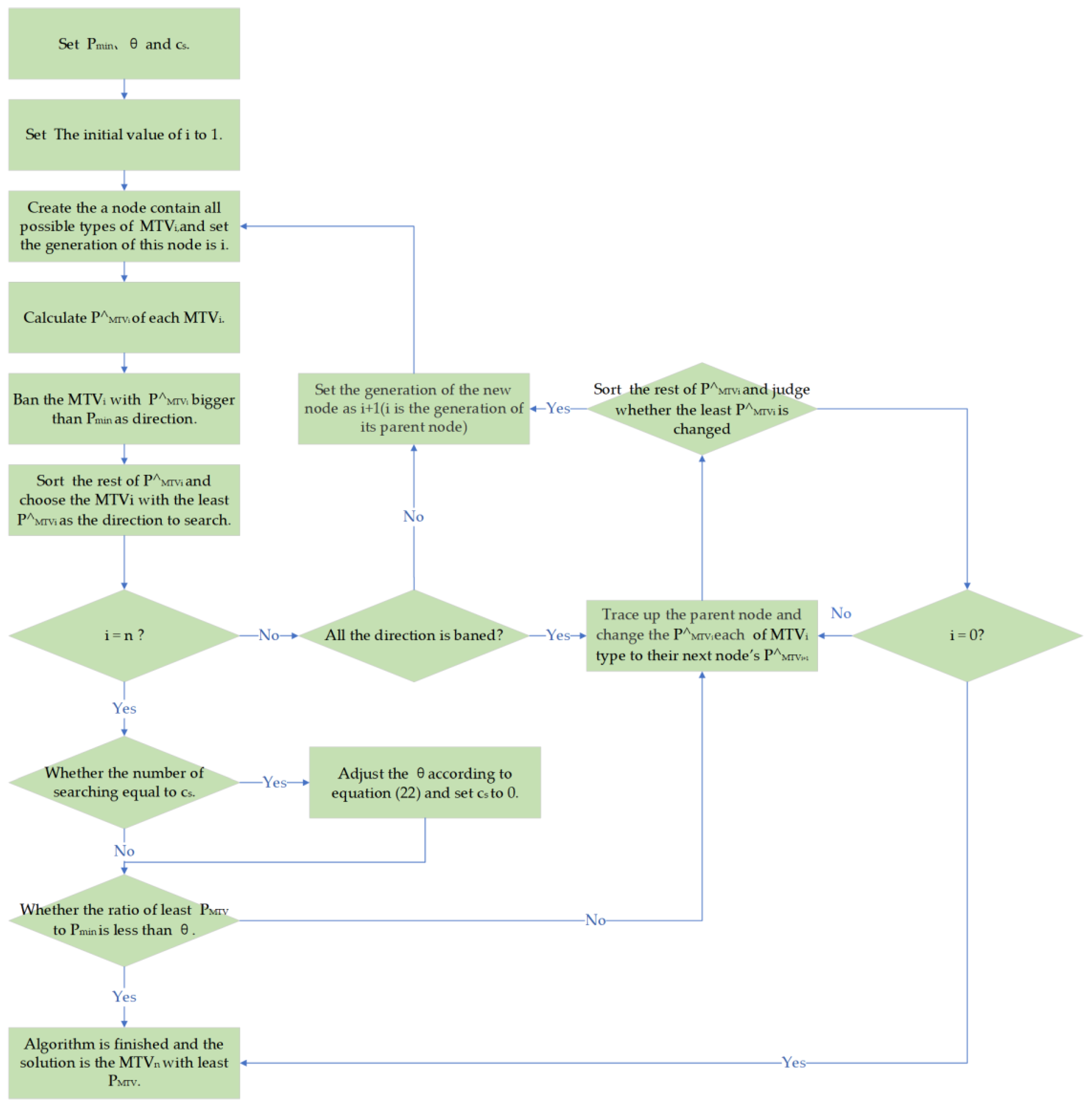
Based on the above improvement, the whole algorithm flow is as follows:

Step 1: According to the P_MTV of the MTVs needed to be optimized, set the $P_{min}, \theta$ and $c_s$.

Step 2: Create the root node of the search tree; the root node contains all possible types of the sub-matrix ${MTV}_1$, each of which corresponds to a search direction.

Step 3: Calculate the ${f(MTV}_1)$ of each type of ${MTV}_1$, then calculate the ${\widehat{P}}_{{MTV}_1}$ of each type of ${MTV}_1$. Ban the direction of those ${MTV}_1$ whose ${\widehat{P}}_{{MTV}_1}$ is bigger than $P_{min}$. Find the ${MTV}_1$ with least ${\widehat{P}}_{{MTV}_1}$ and set it as the direction to expand. Create the next node for ${MTV}_2$, as the same model, and so on, until the node for ${MTV}_n$ is reached.

Step 4: When the number of layers of MTV corresponding to a node is n, it means one search is finished and we obtain a solution. Calculate the $P_{\mathrm{M}\mathrm{T}\mathrm{V}}$ of these ${MTV}_n$s, find the least $P_{\mathrm{M}\mathrm{T}\mathrm{V}}$, and calculate the ratio of $P_{\mathrm{M}\mathrm{T}\mathrm{V}}$ to $P_{min}$. If the ratio is equal to or less than $\theta$, the algorithm ends, and the ${MTV}_n$ with least $P_{\mathrm{M}\mathrm{T}\mathrm{V}}$ is the final solution. Otherwise, if the cumulative number of searches reaches the $c_s$, this algorithm adjusts the $\theta$ by Equation (22).

Step 5: If the algorithm is not finished, trace up the parent node and change the each ${\widehat{P}}_{{MTV}_i}$ of ${MTV}_i$ type to their next node’s ${\widehat{P}}_{{MTV}_{i+1}}$. Find the MTV with the least $P_{\mathrm{M}\mathrm{T}\mathrm{V}}$, and set its direction as the direction needed to expand. If the direction is not changed, continue to trace up. Otherwise, this algorithm will expand in a new direction. If the search tree traces up to the root node, the algorithm ends and, according to the direction of root node, the ${MTV}_n$ with least $P_{\mathrm{M}\mathrm{T}\mathrm{V}}$ is the final solution.

The above steps can be represented by a flow diagram (Figure 6).

The running process of traditional AO* algorithm is a backtracking search process. In the worst case, its time complexity is close to the enumerated type. For the searching of an $n\times m$-scale MTV, the worst time complexity is O ($n!$). The method of this paper introduces adaptive method and depth-first strategy, through observing the result of every $c_s$ searching, the termination condition of the algorithm is adjusted adaptively. The worst time complexity of each searching is $n·{(2}^m-2)$. Under the optimal compactness index, m is up rounding of ${log}_2\left(n+2\right)$. So, the time complexity of this method is O ($c_s·n^2$). The paper’s improvement of AO* algorithm speeds up the efficiency of searching of MTV for large-scale questions, and the process is offline, so it does not affect the actual test efficiency.

4. Experiments and Results

To test our method’s optimization for $P_{MTV}$, this paper used Particle Swarm Optimization Algorithm (PSO), Walk-1 Algorithm, and our method to generate MTVs, and used them to carry out the boundary scan test on the same module under test which is developed by our laboratory. In this test, this paper set the relative error of estimated value of ${\mathrm{P}}_{\mathrm{M}\mathrm{T}\mathrm{V}}$ lower than 10%. The module under test is shown in Figure 7a; it consisted of 3 ICs, including an XC7K325T FPGA, an XC7Z045 FPGA, and a JYCSW1848 CPU. All chips are powered by power modules that allow them to work properly. The circuit under test contains a total of 123 networks and 371 pins. A total of 158 pins of those ICs are connected to the headers, so that testers can inject the shorted-circuit fault they need by using jumper cable to connect the pins of the networks. There are 87 testable networks, covering 71% of all networks. By connecting the JTAG port of the module to our boundary scan test system, which is shown in Figure 7b, testers can do a boundary scan test on it with MTVs generated by this paper.

4.1. P_MTV of Different Algorithms

This paper randomly selects 20 networks from all testable networks and numbers them. Then, this paper calculates their probabilities of shorted circuit by Equation (2). The probabilities are arranged into a matrix in the form of Formula (1), which is shown as

Table 2. The probability of shorted circuit (×10⁻⁵).

Net	1	2	3	4	5	6	7	8	9	10	11	12	13	14	15	16	17	18	19	20
1	0.00	6.37	8.56	6.68	7.98	3.13	5.98	5.18	5.49	2.86	3.24	3.27	5.56	5.89	8.55	5.67	7.66	5.78	6.61	7.92
2	6.37	0.00	4.74	8.15	5.97	1.17	4.88	9.60	4.21	5.33	3.76	8.08	6.63	6.47	7.29	7.24	4.83	3.24	3.15	1.85
3	8.56	4.74	0.00	3.76	7.76	3.72	5.21	5.75	1.50	6.28	5.89	5.36	3.85	4.65	7.37	6.54	2.73	4.47	0.55	6.37
4	6.68	8.15	3.76	0.00	3.47	5.42	6.55	1.89	3.36	6.94	4.13	3.43	3.30	2.43	6.15	3.56	6.09	5.19	9.64	7.08
5	7.98	5.97	7.76	3.47	0.00	6.14	4.08	2.85	3.28	3.95	2.16	4.58	1.65	4.59	5.04	5.60	8.75	6.90	5.07	8.08
6	3.13	1.17	3.72	5.42	6.14	0.00	1.88	3.57	3.85	4.98	5.10	4.29	5.68	8.11	4.20	7.97	9.31	4.46	2.96	5.08
7	5.98	4.88	5.21	6.55	4.08	1.88	0.00	1.08	5.98	3.85	4.46	4.73	4.18	3.90	3.10	0.67	4.09	8.17	4.23	2.83
8	5.18	9.60	5.75	1.89	2.85	3.57	1.08	0.00	6.78	5.09	5.99	1.53	7.02	3.49	5.04	5.80	9.94	6.32	7.59	8.55
9	5.49	4.21	1.50	3.36	3.28	3.85	5.98	6.78	0.00	6.57	9.10	4.84	1.92	6.49	1.55	3.38	1.83	1.46	6.01	8.25
10	2.86	5.33	6.28	6.94	3.95	4.98	3.85	5.09	6.57	0.00	4.65	4.07	2.96	4.94	4.83	2.21	3.16	4.95	5.35	4.57
11	3.24	3.76	5.89	4.13	2.16	5.10	4.46	5.99	9.10	4.65	0.00	3.15	4.27	6.89	1.75	5.36	2.69	4.50	4.18	6.34
12	3.27	8.08	5.36	3.43	4.58	4.29	4.73	1.53	4.84	4.07	3.15	0.00	4.36	4.50	5.24	4.98	8.53	6.56	4.02	5.77
13	5.56	6.63	3.85	3.30	1.65	5.68	4.18	7.02	1.92	2.96	4.27	4.36	0.00	4.38	5.07	6.54	8.51	2.90	4.52	7.18
14	5.89	6.47	4.65	2.43	4.59	8.11	3.90	3.49	6.49	4.94	6.89	4.50	4.38	0.00	4.13	6.23	2.95	4.91	2.84	5.36
15	8.55	7.29	7.37	6.15	5.04	4.20	3.10	5.04	4.20	3.10	5.04	1.55	4.83	4.13	0.00	5.53	3.81	4.62	3.97	9.25
16	5.67	7.24	6.54	3.56	5.60	7.97	0.67	5.60	7.97	0.67	5.80	3.38	2.21	5.36	5.53	0.00	5.04	1.83	5.26	3.31
17	7.66	4.83	2.73	6.09	8.75	9.31	4.09	8.75	9.31	4.09	9.94	1.83	3.16	2.69	8.53	5.04	0.00	2.46	3.20	4.03
18	5.78	3.24	4.47	5.19	6.90	4.46	8.17	6.90	4.46	8.17	6.32	1.46	2.90	4.91	4.62	1.83	2.46	0.00	7.73	6.83
19	6.61	3.15	0.55	9.64	5.07	2.96	4.23	5.07	2.96	4.23	7.59	6.01	4.52	2.83	3.97	5.26	3.20	7.73	0.00	6.09
20	7.92	1.85	6.37	7.08	8.08	5.08	2.83	8.55	8.25	4.57	6.34	5.77	7.18	5.36	9.25	3.31	4.03	6.83	6.09	0.00

.

After the probability of shorted circuit is obtained, according to the description in Section 3.4; this paper used the improved genetic algorithm to determine the parameters ${\beta }_k$ of the heuristic function in GA-AO* approach. This paper set $c_{end}$ to 5000. After iteration, the final value of ${\beta }_k$ is shown in

Table 3. Actual values of ${\beta }_k$.

k	1	3	4	5	6	7	8	9	10	11	12	13
Value $({10}^{-4})$	1.157	2.076	0.211	0.007	0.273	2.678	0.001	0.002	0.001	0.002	0.001	0.001

.

The estimated $P_{\mathrm{M}\mathrm{T}\mathrm{V}}$ and actual $P_{\mathrm{M}\mathrm{T}\mathrm{V}}$ under each order of sub-matrix is shown in Figure 8, with an average relative error of 6.9%. The results show that our heuristic function has good estimation ability for $P_{\mathrm{M}\mathrm{T}\mathrm{V}}$.

This paper used these three algorithms to generate MTVs according to the probability of shorted circuit in Table 2. The codes of these algorithms were implemented on MATLAB 2020. The CPU type of the computer running codes was “Intel (R) Core (TM) i7-10750H CPU@2.60 GHz”. All algorithms generated MTVs for the same networks under optimal compactness, which means this paper set the number of columns of MTVs as the rounding up of ${log}_2(n+2)$ (n is the number of networks under test). This paper set the $P_{\mathrm{M}\mathrm{T}\mathrm{V}}$ of MTVs which is generated by PSO as the initial value of $P_{min}$. Finally, this paper set $\theta$ to 80% and $c_s$ to 100. PSO and Walk-1 are implemented according to the ways and parameters provided in reference [16] and reference [17], respectively. Under these conditions, this paper observed the changes of $P_{\mathrm{M}\mathrm{T}\mathrm{V}}$ of the three algorithms by changing the number of networks under the boundary scan test and evaluated the $P_{\mathrm{M}\mathrm{T}\mathrm{V}}$. When the number of networks is 5, 10, 15, and 20, respectively, the $P_{\mathrm{M}\mathrm{T}\mathrm{V}}$ of the MTVs generated by three algorithms are shown in

Table 4. The $P_{\mathrm{M}\mathrm{T}\mathrm{V}}$ of each algorithm under different number of networks under test.

Number of Networks	Walk-1	PSO	Our Method
5	0	$3.47\times {10}^{-5}$	0
10	$6.05\times {10}^{-4}$	$4.10\times {10}^{-4}$	$1.85\times {10}^{-4}$
15	0.0024	0.0016	$3.16\times {10}^{-4}$
20	0.0068	0.0030	0.0021

.

The $P_{\mathrm{M}\mathrm{T}\mathrm{V}}$ of the MTVs generated by the three algorithms varies with the number of networks as shown as Figure 9.

As can be seen from Table 4 and Figure 9, all three algorithms can generate fault-free MTVs when the number of networks is small. With the increase in network size, the $P_{\mathrm{M}\mathrm{T}\mathrm{V}}$ of MTV generated by Walk-1 algorithm increases significantly because of fixed compactness index, while the MTVs generated by PSO and by our method can still maintain a low $P_{\mathrm{M}\mathrm{T}\mathrm{V}}$. At the same time, because we take the $P_{\mathrm{M}\mathrm{T}\mathrm{V}}$ of the MTVs generated by the PSO as $P_{min}$ of our method, the $P_{\mathrm{M}\mathrm{T}\mathrm{V}}$ of the MTVs generated by our method is always less than or equal to the $P_{\mathrm{M}\mathrm{T}\mathrm{V}}$ of the MTVs generated by the PSO, so our method realizes the optimization. When the number of networks is 20, the running time of the three algorithms is 0.074 s, 248 s, and 1756 s. For the actual test, the generation of MTV for the same type of circuit is one-time and offline, so the generation time of MTV will not affect the test efficiency basically.

4.2. Test Performance of Different Algorithms

In order to test the performance of MTVs generated by three algorithms in the actual boundary scan test, we actually inject these faults into the module under test by connecting the corresponding jumper cables and using the MTVs generated by these three algorithms to do the boundary scan test on it. We use the method of weighted sampling to extract the shorted-circuit fault to be injected from Figure 4. Each time, we will extract one or two faults to simulate the 2-order and the 3-order short-circuit fault. The weight of a 2-order or a 3-order short-circuit fault is the ratio of the probability of it and the sum of all the probabilities of all the 2-order and 3-order shorted faults. After injecting the faults extracted, we connect the JTAG of the module to our boundary scan test system EasyScan-USB IEEE 1149.1 and use the system to inject the MTVs. For each algorithm, we do the 200 experiments. The rates of misjudgment or confusion in the test using MTVs generated by each algorithm are shown in

Table 5. The rates of misjudgment or confusion in the test using MTVs generated by each algorithm.

Number of Tests	Walk-1	PSO	Our Method
50	48.3%	34.1%	27.4%
100	44.1%	33.2%	26.5%
150	47.6%	34.3%	26.6%
200	45.7%	34.1%	26.3%

. The results show that the MTVs generated by our method are less frequently misjudged or confused than those generated by walk-1 and PSO. It shows, from a posterior perspective, that our MTVs have a lower failure rate when tested.

5. Conclusions

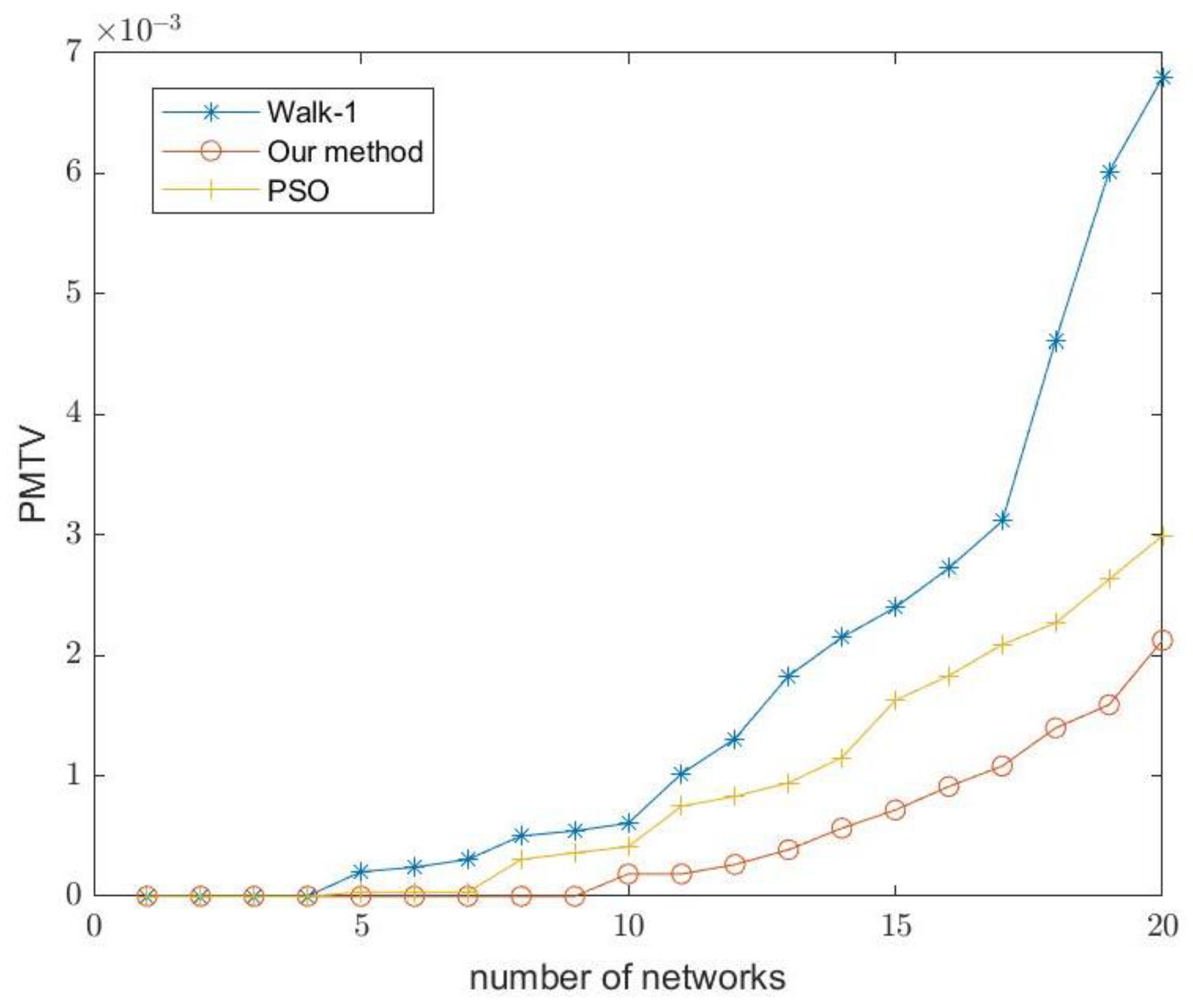
In this paper, a method of generating boundary-scan MTV by combining the genetic algorithm and improved AO* model is proposed, which effectively solves the problem of optimizing the $P_{\mathrm{M}\mathrm{T}\mathrm{V}}$ of MTV under the optimal compactness index. We use walk-1, PSO, and our method to generate MTVs for the same module and calculate the $P_{\mathrm{M}\mathrm{T}\mathrm{V}}$ of each MTV. At the same time, we also used these MTVs for the actual boundary scan test. Based on the analysis and experiments, we can draw the following conclusions:

• Compared with the MTVs generated by Walk-1 and PSO, the MTVs generated by our method have lower P_MTV, and MTVs generated by our method have lower apriorism probability of misjudgment and confusion in the boundary scan test.
• Through the experiment of fault injection based on probability of shorted circuit, it is shown that the MTVs generated by our method have lower fault incidence than those generated by walk-1 and PSO. The MTVs generated by our method have lower failure rate from a posteriori point of view.

Our research can be used to generate MTV in the boundary scan test and to optimize the $P_{\mathrm{M}\mathrm{T}\mathrm{V}}$ of existing MTVs. It has certain practical value. In the future, we will do more research on the generation of larger MTVs and adaptive optimization with failure rate and compactness.