A Study on the Surrogate-Based Optimization of Flexible Wings Considering a Flutter Constraint ^†

Abstract

Accounting for aeroelastic phenomena, such as flutter, in the conceptual design phase is becoming more important as the trend toward increasing the wing aspect ratio forges ahead. However, this task is computationally expensive, especially when utilizing high-fidelity simulations and numerical optimization. Thus, the development of efficient computational strategies is necessary. With this goal in mind, this work proposes a surrogate-based optimization (SBO) methodology for wing design using a predefined machine learning model. For this purpose, a custom-made Python framework was built based on different open-source codes. The test subject was the classical Goland wing, parameterized to allow for SBO. The process consists of employing a Latin Hypercube Sampling plan and subsequently simulating the resulting wing on SHARPy to generate a dataset. A regression-based machine learning model is then used to build surrogate models for lift and drag coefficients, structural mass, and flutter speed. Finally, after validating the surrogate model, a multi-objective optimization problem aiming to maximize the lift-to-drag ratio and minimize the structural mass is solved through NSGA-II, considering a flutter constraint. This SBO methodology was successfully tested, reaching reductions of three orders of magnitude in the optimization computational time.

1. Introduction

The need to account for aeroelastic phenomena, namely, flutter, during the conceptual design phase has gained relevancy as wing designs become slenderer to reduce the induced drag [1]. However, this need comes with a computational challenge, especially when integrated into a Multidisciplinary Design Optimization (MDO) [2] environment to perform Fluid–Structure Interaction (FSI) simulations to estimate flutter speed. Therefore, searching for more computationally efficient solutions that are able to maximize wing performance without reaching flutter within the flight envelope is required. With this goal in mind, different approaches are considered in the literature, namely, multi-fidelity models [3,4], conventional [5] and machine learning-based surrogate models [6], and reduced-order models [7].

Low-fidelity (LF) [8], high-fidelity (HF) [9,10], and multi-fidelity (MF) [11,12] models have all been tested in different flutter-constrained MDO problems of wings. These models span from LF models such as potential flow theory and panel methods with corrections [8,11,12], accounting for both compressibility and viscous effects, to Euler [11] and HF Reynolds-Averaged Navier–Stokes (RANS) solvers [9,10,12]. Most of these optimization problems were aimed at maximizing range [8,9,11], although fuel burn [12] and structural mass [10] minimization has also been chosen.

Even though reduced-order and surrogate models have been applied to aeroelasticity problems for some time [13], especially to study unsteady nonlinear aeroelasticity problems that arise from unconventional features such as limit-cycle oscillations [14,15,16], their usage for MDO problems considering flutter is scarce [17,18,19] in the open literature, particularly for MDO problems considering aerodynamic performance and structural weight. For instance, Sohst et al. [17] developed an MDO strategy that uses multi-fidelity solvers and surrogate models to design strut-braced and high-aspect-ratio wings considering flutter and stress constraints. They found that, although the flutter constraint was respected in the optimization process, unaccounted buckling was observed in a nonlinear assessment of the optimized strut-braced wing aircraft design. Cea and Palacios [18] implemented an optimization framework based on ROMs that couples different open-source codes, including SHARPy, for minimizing the mass of a flexible strut-braced wing while accounting for flutter speed as a constraint. Toffol and Ricci [19] developed a methodology combining in-house codes with surrogate models to optimize the structural layout of a conventional aircraft such that its mass is minimized while considering stress and flutter constraints. The application of surrogate models based on machine learning is scarcer. Nevertheless, this research field is starting to emerge, particularly for aerodynamics [6,20].

In this work, a surrogate-based optimization (SBO) strategy is presented to conceptually design flexible wings based on machine learning-based surrogate models with the aim of maximizing aerodynamic performance, minimizing structural mass, and satisfying the flutter constraint.

2. Methodology

The methodology employed in this work and depicted in Figure 1 adheres to three fundamental steps commonly found in SBO: (i) dataset definition and generation; (ii) surrogate model training, validation, and testing; and (iii) the optimization process. All these tasks were performed using available open-source Python codes and specially developed Python scripts. For illustrative purposes, the methodology is applied for a cruise speed of 30 m/s, but it is applicable to other speeds.

Firstly, the Goland wing [21] was selected to be the baseline model for this work. The reason for this choice was two-fold: (i) experimental data exist to validate the implementation; (ii) it has been already used to validate SHARPy [22], the open-source code chosen for the aeroelastic simulations and developed by Imperial College London. SHARPy provides a coupled aeroelastic solution considering the Unsteady Vortex Lattice Method (UVLM) [23] and Geometrically Exact Beam Model (GEBM) [24] for aerodynamic and structural analyses, respectively. Krylov and modal projections are used in SHARPy to linearize aerodynamic and structural subsystems, respectively. These are then used to estimate the flutter speed by means of the iterative p-k method at the nonlinear aeroelastic equilibrium. The flutter speed was predicted in the SHARPy implementation used for this work to be under 5% of the relative error for the Goland wing, in agreement with the value obtained by SHARPy developers [25]. To improve the accuracy of the drag estimation, the flat-plate theory [26] was implemented, offering an estimation of skin-friction drag multiplied by form (more adequate for small angles of attack) and interference factors. Currently, there are some efforts being made by the SHARPy team [27,28] to include viscous considerations in the UVLM, which are typically not of major importance when the focus is on aeroelastic phenomena.

2.1. Dataset Definition and Generation

2.1.1. Design Space

In regard to the design variables, the choice rested on four key parameters in aeroelasticity: wing aspect ratio (AR), sweep angle ($\Lambda$), torsional stiffness ($GJ$), and angle of attack ($\alpha$). The AR is vital to improve aerodynamic efficiency and fuel consumption, although it poses aeroelastic and structural challenges [1]. The sweep angle ($\Lambda$) influences transonic flow onset and aircraft aeroelastic stability [29]. $GJ$ relates how wings respond to aerodynamic loads and is critical to averting aeroelastic instabilities [29]. Lastly, $\alpha$ impacts lift and drag, affecting flight stability. Besides their relevancy to and impact on the aeroelastic behavior, SHARPy’s ability to modify these variables without coding was fundamental in their selection. The upper and lower boundaries (UB and LB, respectively) of these parameters are listed in

Table 1. The design variables and respective boundaries used for the dataset generation and optimization problem.

DVs	Initial	LB	UB	Units
AR	6.67	6	16	-
$\Lambda$	0	0	40	deg
GJ	0.99 × ${10}^6$	0.70 × ${10}^6$	1.70 × ${10}^6$	N.m2
$\alpha$	0.05	–5	15	deg

alongside the initial values that correspond to the Goland wing specifications. These boundaries were later adjusted based on the preliminary optimization results.

2.1.2. Sampling Plan

For sampling, Latin Hypercube Sampling (LHS) was adopted using the pyDOE2 package [30] due to its uniform coverage across the design space and its efficient sampling scheme. Simulations conducted in SHARPy focused on the wing metrics to be used in the optimization: structural mass, flutter speed, and aerodynamic coefficients ($C_L$ and $C_D$). For this study, 2000 simulation samples were generated. Despite this number appearing to be modest given the complexity of the problem, the high computational demands of SHARPy made this a significant effort. Each simulation averaged around 93.5 s. The simulations were run on a host computer with Windows 11, an Intel i7-10510U processor, 16 GB DDR4 RAM, and a 477 GB SSD. This machine also used NVIDIA GeForce MX250 graphics. Within this system, a virtual machine operated on Ubuntu 22.10, utilizing 4 cores, 11 GB RAM, and 59.2 GB of storage space. Virtualization was facilitated by Oracle VM VirtualBox 7.0.6.

2.2. Surrogate Model Training, Validation, and Testing

This subsection provides an overview of surrogate model development, from training to testing. The goal is to find a machine learning-based surrogate model that meets computational needs and offers a high predictive accuracy. Our criteria for selecting the model include accuracy, efficiency, and robustness.

We considered various regression-based machine learning models from the scikit-learn Python library [31], including Bayesian Ridge, Decision Tree Regressor, Extra Trees Regressor, Lasso, ARD Regression, and Linear Regression. For the model generation, we considered a 60%–30%–10% split for training, validation, and testing, respectively, based on experimenting with different combinations for generating surrogates of $C_L$, $C_D$, mass, and flutter speed. A random procedure was followed to assign the data points to each set. These machine learning models were set with random hyperparameters to gauge their baseline performance. Each was then assessed on the validation subset.

The methods were evaluated for flutter speed, mass, drag, and lift coefficients, i.e., the output parameters from SHARPy that were used for the optimization problem definition. All the considered models were able to well represent the structural mass, drag, and lift coefficients, with values of R² higher than 0.99 and of Root Mean Squared Error (RMSE) lower than 1%. However, the models evidenced difficulty in provide accurate predictions of flutter speed, as shown in

Table 2. Flutter speed performance metrics.

Method	R2 (-)	RMSE (%)
Extra Tree Regressor	0.921	8.92
Decision Tree Regressor	0.749	15.84
Linear Regression	0.245	27.5
Bayesian Ridge	0.245	27.5
Lasso	0.244	27.5
ARDR Regression	0.243	27.5

.

While, for this model, only the Decision Tree method approached the performance of Extra Trees (still remaining inferior), for the other models, the difference between the methods was minimal. With these considerations in mind and for consistency and simplicity in the workflow, we chose to use the Extra Trees Regressor as the surrogate model method for all output variables. After determining the Extra Trees Regressor’s aptitude, the training and validation processes began.

Alternatively, another SBO strategy could be explored in the future, where new infill points are added alongside the optimization using an appropriate acquisition function and Bayesian Optimization [32]. This approach was recently applied to an aero-structural problem by Cardoso et al. [33].

2.2.1. Training and Validation

The model was trained using the dataset, focusing on hyperparameter tuning. Hyperparameters were carefully adjusted to ensure model accuracy and prevent overfitting. The optimal settings were identified via a Grid Search, using RMSE and R² for selection. The model’s hyperparameters analyzed were the number of trees in the ensemble, maximum tree depth, minimum samples at a leaf node, and minimum samples for a node split [34]. The objective during training is to minimize a loss function for improved prediction based on input data, ensuring that hyperparameters are set for both known (training set) and unseen (validation set) data.

2.2.2. Testing

After training and validation, the model is tested on a dataset it has not seen before, known as the test set, to gauge the model’s effectiveness. Learning curves further evaluate the model’s generalization. The final surrogate models used for testing and the later optimization process are based on the optimal hyperparameters obtained for each model after tuning. The suitability of surrogate models for the aeroelastic analyses required for the optimization process was visualized using parameters from the testing dataset. The results for each model are shown in Figure 2.

From the results, the surrogate models accurately predict the mass and lift coefficient. Discrepancies in the drag coefficient suggest complexities in aeroelastic interactions in certain regions of the design space. The flutter speed showed the greatest difference, with an R² of 0.921. The flutter model might have been overfitting, as can be seen from the learning curves in Figure 3, and more data might improve its performance. Challenges in flutter modeling could arise from estimating flutter speed using the iterative p-k method.

2.3. Optimization Process

The last step in the implemented SBO methodology is to solve the optimization problem, which is a multi-objective one, as we want to maximize aerodynamic performance in terms of the lift-to-drag ratio ($C_L/C_D$) and minimize structural mass while ensuring that the flutter speed ($V_{\mathrm{flutter}}$) is far from the cruise speed ($V_{\mathrm{cruise}}$). Mathematically, the optimization problem can be stated as follows:

$$\begin{array}{cccc}\hfill & \mathrm{minimize}\hfill & \hfill & f\left(-C_L/C_D,\mathrm{mass}\right)\hfill \\ \hfill & \mathrm{with}\mathrm{respect}\mathrm{to}\hfill & \hfill & x=(\mathrm{AR},\Lambda ,GJ,\alpha )\hfill \\ \hfill & \mathrm{subject}\mathrm{to}\hfill & \hfill & c=V_{\mathrm{cruise}}-\left(V_{\mathrm{flutter}}/1.5\right)\le 0\hfill \end{array},$$

(1)

where f, x, and c denote the classical notation for objective functions, the design variable set, and constraints, respectively. The factor 1.5 provides a safety factor against flutter, a standard in aerospace engineering [35]. Since this is a multi-objective problem and the run time of the surrogate model is inexpensive, a gradient-free optimizer was chosen to better explore the design space, namely, the implementation of Non-dominated Sorting Genetic Algorithm II (NSGA-II) [36] in pygmo [37]. However, as NSGA-II is an unconstrained optimization algorithm, a penalty was added to the objective function when the flutter constraint is not respected.

In this work, the population size, mutation rate, and crossover rate were adjusted to improve the resulting Pareto front while ensuring a good balance between the computational cost, hypervolume, and ranking. It is worth mentioning that hypervolume measures the space occupied by solutions in the target space, while ranking helps select solutions based on levels of non-dominance [36].

After obtaining the Pareto fronts with the initial design variable boundaries (Table 1), a significant discrepancy was noted in some results. A concentration of solutions was found near the lower limit for the sweep angle and torsional stiffness, as can be observed in Figure 4, suggesting that extending these limits might produce better solutions. In addition, surrogate models showed high prediction errors for high aspect ratios.

To solve this problem, the boundaries of the design variables were extended and the dataset was augmented, focusing particularly on the critical aspect ratio interval. An iterative analysis and modification of the dataset show a systematic approach to addressing optimization challenges, emphasizing the importance of identifying weaknesses in the model and making necessary changes.

3. Results

The outcomes of the optimization procedures for three cruise speeds are examined in this section. Using surrogate models for design optimization, optimal solutions are derived and then compared to reference results from SHARPy simulations.

3.1. Case 1: Cruise Speed of 30 m/s

The first cruise speed considered was 30 m/s. Initially, an optimization was performed with a specific set of parameters obtained by tuning, and the solutions were compared with SHARPy simulations. Even though the results were accurate, especially for $C_L$, $C_D$, and mass, they evidenced discrepancies in flutter velocity estimation as mentioned previously and presented in Table 2. To solve this problem, the boundaries of the design variables were expanded, as explained in the previous section, adding more data points to improve the accuracy of the prediction. A new optimization with the updated data showed a reduced error for most parameters. The final surrogate models were built based on a dataset of 2500 points with the metrics shown in

Table 3. Final RMSE and R² metrics for Case 1 (cruise speed of 30 m/s).

Model	RMSE (%)	R2 (-)
Flutter speed	7.276	0.952
Mass	0.293	0.999
$C_D$	0.0006	0.998
$C_L$	0.0059	0.999

.

However, to further improve accuracy, more computational resources were allocated. Increasing the population size from 180 to 280 and the number of generations from 50 to 200 improved the flutter speed estimation, confining the metric deviations within a 5% margin of error, as can be observed in

Table 4. Optimized solutions obtained with the surrogate models compared to the corresponding SHARPy results for Case 1 (cruise speed of 30 m/s).

Objective	Metric	SHARPy	Optimization	Relative Difference
	$C_L/C_D$	39.83	39.79	0.09%
$C_L/C_D$ maximization	Mass	1043.57 kg	1043.46 kg	0.01%
	Vflutter	133.65 m/s	127.89 m/s	4.30%
	$C_L/C_D$	26.37	27.13	2.85%
Mass minimization	Mass	313.84 kg	392.17 kg	0.08%
	Vflutter	188.41 m/s	188.10 m/s	0.16%

. Yet, this came at the cost of computational efficiency, with a five-fold increase in computational time.

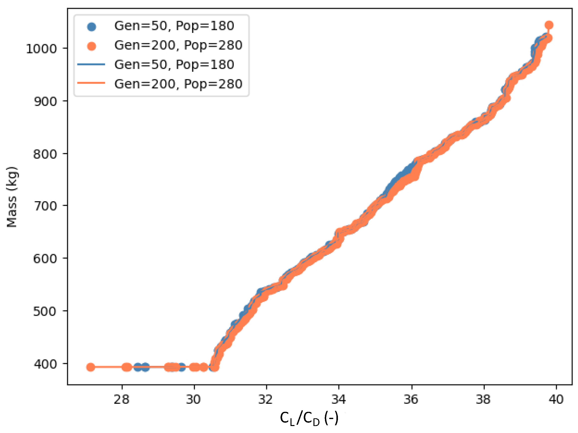
Pareto front analysis revealed trade-offs between the two optimization objectives. The extended configuration covered a wider Pareto range, suggesting its ability to explore a complete solution space and produce better results, particularly toward higher $C_L/C_D$ values, as can be seen in Figure 5.

Throughout the study, the flutter constraint remained inactive, prompting further investigation of the Goland wing’s behavior at higher cruise speeds.

3.2. Case 2: Cruise Speed of 60 m/s

For Case 2, the optimization was conducted at a cruise speed of 60 m/s using the same methodology as the one applied for 30 m/s. The Extra Trees Regressor was identified as the best surrogate model, with the performance metrics presented in

Table 5. Final RMSE and R² metrics for Case 2 (cruise speed of 60 m/s).

Model	RMSE (%)	R2 (-)
Flutter speed	7.360	0.913
Mass	0.377	0.999
$C_D$	0.0034	0.947
$C_L$	0.013	0.999

.

For a cruise speed of 60 m/s, from 9000 combinations, the flutter constraint was active only 0.322% of the time. The design variables for which the flutter constraint was active fell within the following specific ranges: AR of 15.2–15.4; $\Lambda$ of 10.4–11.3 degrees; $GJ$ between 1.62 × 10⁶ and 1.70 × 10⁶ N.m²M; and $\alpha$ of 6.86–6.95 degrees.

Nevertheless, the optimization algorithm found 180 optimal solutions where the flutter constraint was never active. These solutions differed in design variables from those where the flutter phenomenon was a concern. A subsequent, more detailed analysis aimed to reduce the relative error to under 5% for all outcomes.

The results in

Table 6. Optimized solutions obtained with the surrogate models compared to the corresponding SHARPy results for Case 2 (cruise speed of 60 m/s).

Objective	Metric	SHARPy	Optimization	Relative Difference
	$C_L/C_D$	36.08	36.16	0.21%
$C_L/C_D$ maximization	Mass	927.40 kg	927.06 kg	0.04%
	Vflutter	91.94 m/s	92.23 m/s	0.32%
	$C_L/C_D$	21.28	21.56	1.32%
Mass minimization	Mass	392.62 kg	392.32 kg	0.08%
	Vflutter	194.92 m/s	188.92 m/s	3.08%

show that all percentage errors were below the threshold after a deeper exploration of the design space and an increase in the optimization parameters, as was implemented for the 30 m/s analysis.

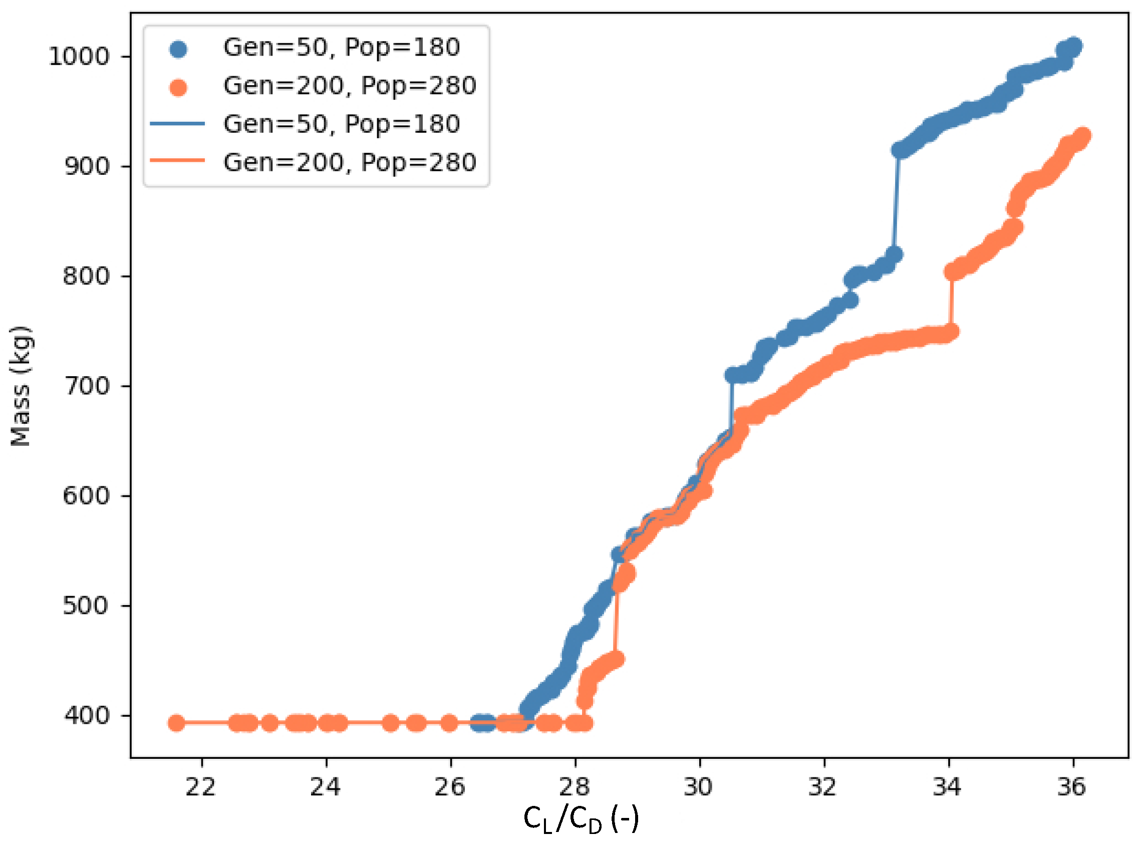
However, this intensive optimization resulted in a 491% increase in computational time. Nevertheless, the potential for greater accuracy seems to justify the additional computational effort. Comparing the Pareto fronts in Figure 6, an improvement was evident, especially at higher $C_L/C_D$ values. In these cases, the advanced optimization provided better aerodynamic efficiency with a lower mass increase. However, for some design choices, there was a significant overlap in results between the initial and advanced optimizations, indicating that increasing iterations and population sizes do not always lead to different results.

3.3. Case 3: Cruise Speed of 130 m/s

For the final case, considering a cruise speed of 130 m/s, the flutter phenomenon emerged for most of the points in the dataset, which made optimization difficult. The performance of the surrogate models on which the optimization was based is shown in

Table 7. Final RMSE and R² metrics for Case 3 (cruise speed of 130 m/s).

Model	RMSE (%)	R2 (-)
Flutter speed	7.981	0.907
Mass	0.263	0.999
$C_D$	0.0017	0.997
$C_L$	0.011	0.999

.

The initial optimization process, despite using an expanded dataset, produced results with high percentage errors compared with SHARPy, especially in terms of $C_L/C_D$ and flutter velocity. This was primarily due to the active flutter constraint in a vast majority (82.2%) of the examined design combinations that led to the introduction of a penalty in the objective function. Consequently, in the Pareto front of 180 optimal solutions, 24.4% had active flutter issues. To address this, the optimization was reevaluated by increasing the population size to 280 and the number of generations to 200, as was implemented for the previous cruise speeds.

The modified approach yielded a substantial reduction in the number of solutions with an active flutter constraint, down to 7.5%. However, this improvement came at a significant computational cost, with a 690% increase in time compared to the initial optimization. Despite the improvement, the percentage errors were still remarkably high, and the Pareto fronts showed several infeasible solutions due to the active flutter problem and the penalties associated with the results.

However, a closer examination of the results, focusing particularly on the solutions not affected by flutter, showed commendable accuracy. For the most exhaustive optimization (with 200 generations and a population of 280), errors were consistently less than 5%, as listed in

Table 8. Optimized solutions obtained with the surrogate models compared to the corresponding SHARPy results for Case 3 (cruise speed of 130 m/s).

Objective	Metric	SHARPy	Optimization	Relative Difference
	$C_L/C_D$	13.12	13.71	4.47%
$C_L/C_D$ maximization	Mass	1030.99 kg	1030.06 kg	0.03%
	Vflutter	189.21 m/s	194.87 m/s	2.96%
	$C_L/C_D$	11.99	12.37	3.14%
Mass minimization	Mass	955.82 kg	956.41 kg	0.06%
	Vflutter	188.82 m/s	195.03 m/s	3.29%

.

These results, in line with those obtained for the cruise speeds previously examined, clearly reveal that the high penalties were the main cause of the high percentage errors previously observed.

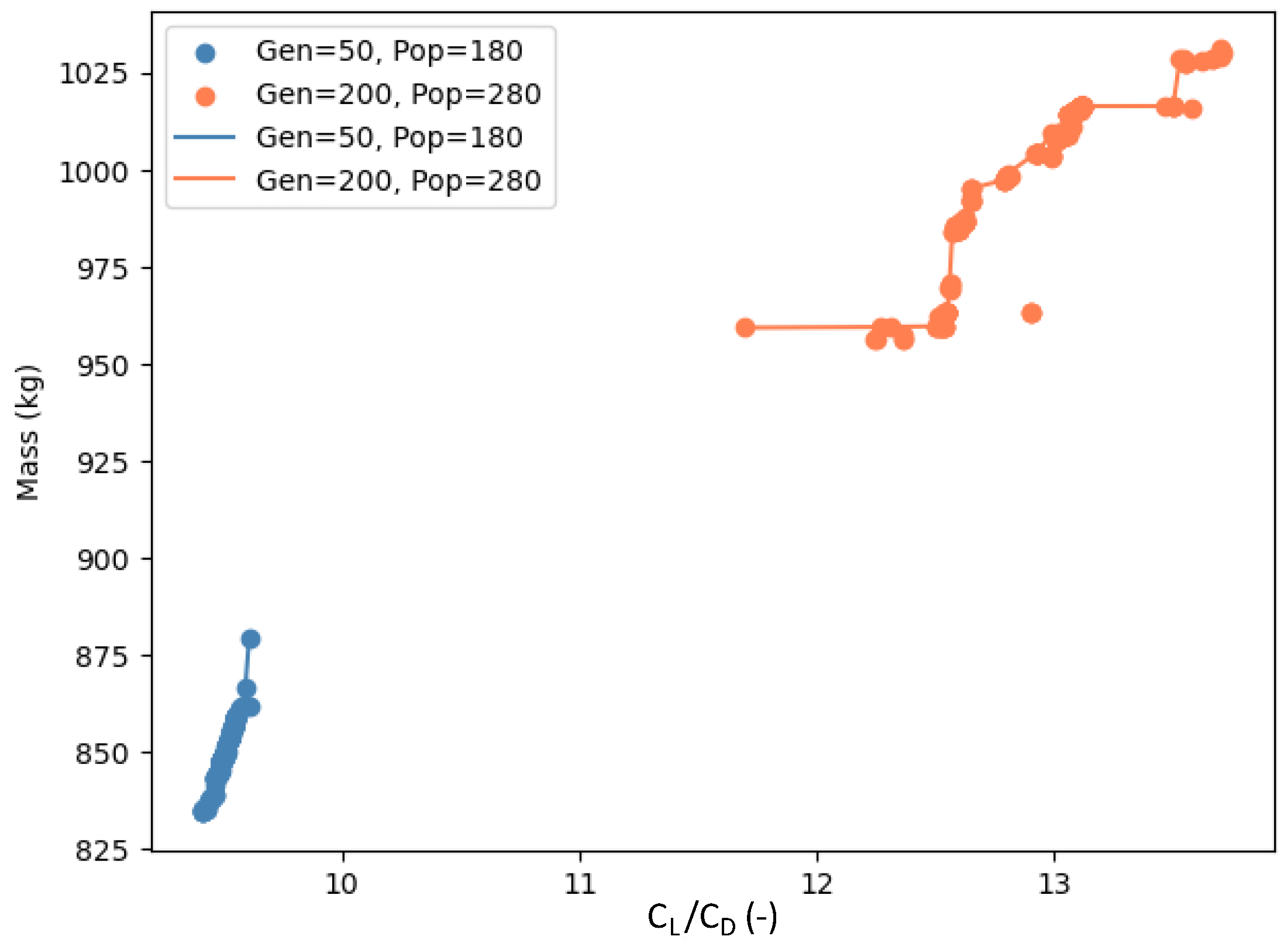
Two distinct groups of solutions can be immediately identified from the graph in Figure 7. In both cases, the optimized design space is significantly reduced, but the second offers a more diverse set of solutions.

Moreover, considering only the feasible solutions, we obtained results that are aligned with the previous cases. This further strengthens the viability of the implemented SBO strategy and shows that, despite the obstacles represented by penalties, the algorithm is able to offer very good solutions.

3.4. Comparison and Discussion of the Results

A final comparison is presented in

Table 9. Optimization results across the analyzed cruise speeds.

${\mathit{V}}_{\mathbf{cruise}}$ (m/s)	Objective	${\mathit{C}}_{\mathit{L}}/{\mathit{C}}_{\mathit{D}}$ (-)	Mass (kg)	AR (-)	$\mathbf{\Lambda }$ (deg)	$\mathbf{GJ}$ (N.m2)	$\mathit{\alpha }$ (deg)	Vflutter (m/s)
30	$C_L/C_D$ maximization	39.79	1043.46	15.97	–2.10	1.54 × 106	4.27	127.89
	Mass minimization	27.13	392.17	6.00	28.7	1.36 × 106	5.13	188.10
60	$C_L/C_D$ maximization	36.16	927.06	14.20	0.72	1.61 × 106	6.14	92.23
	Mass minimization	21.56	392.32	6.00	32.92	7.38 × 105	7.03	188.92
130	$C_L/C_D$ maximization	13.71	1030.06	15.78	6.66	9.37 × 105	9.12	194.87
	Mass minimization	12.37	956.41	14.65	7.24	8.80 × 105	10.39	195.03

, which details the results obtained using consistent parameters and dataset sizes across the three analyzed cruise speeds. The following optimization parameters were set: a population size of 280; 200 generations; a mutation rate of 0.5; and a crossover rate of 0.8. For the last analysis, using a cruise speed of 130 m/s, the results considered are just the feasible ones, i.e., those without the flutter constraint active.

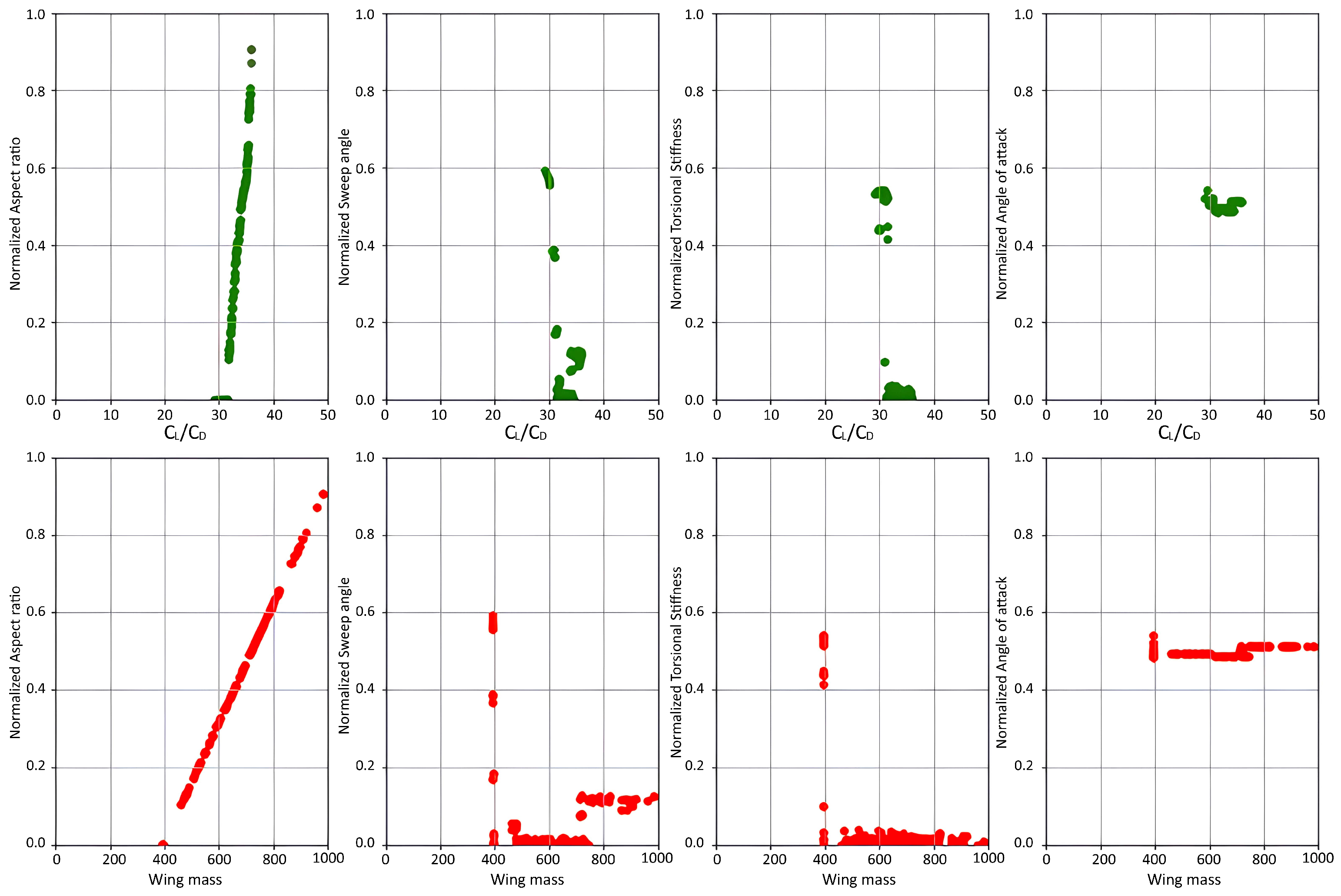
Firstly, one can notice that, as expected, when improving one parameter, the other worsens accordingly, typical of the nature of multi-objective optimization. High values of $C_L/C_D$ consequently correspond to higher mass values.

It is possible to observe that the aspect ratio is consistently higher when maximizing $C_L/C_D$ compared to minimizing the mass across all cruise speeds. This observation aligns with established aerodynamic principles: wings with a higher AR have longer spans relative to their chord, which reduces the induced drag and consequently improves the lift-to-drag ratio. However, the flip side of this advantage is that longer, slenderer wings tend to be more flexible. Indeed, it is possible to observe how the flutter phenomenon in this case occurs at lower speeds. To counterbalance this issue, these wings are heavier and require a higher torsional stiffness to comply with the flutter speed constraint. Deviating from the usual trend is the relatively high aspect ratio observed at the highest cruise speed for the mass minimization objective. This unexpected outcome may be attributed to the narrower feasible design space identified by the surrogate model, and the optimizer that might have been trapped in a local minima region.

At the lower cruise speeds (30 m/s and 60 m/s), when the primary objective is to minimize mass, a positive and more pronounced sweep angle is observed. This might be associated with a structural benefit, redistributing the lift toward the root, which can result in a lighter wing structure. However, when maximizing $C_L/C_D$, a lower sweep may favor aerodynamic efficiency at these speeds.

Variations in torsional stiffness and the angle of attack across the different objectives and velocities are subtler compared to other parameters. However, it is worth noting that higher $C_L/C_D$ values are associated with lower angles of attack. This trend aligns with the expectation that a reduced angle of attack would lead to decreased aerodynamic drag. Lowering the angle of attack while still achieving adequate lift is a strategy to enhance the aerodynamic efficiency of the wing.

Another important observation about the aspect ratio is that for both 30 m/s and 60 m/s cruise speeds, the optimal solutions approach the boundaries of the defined design space, which was set between 6 and 16. This is significant, as it indicates that the design space might not fully encompass the optimal regions for these objectives at these speeds.

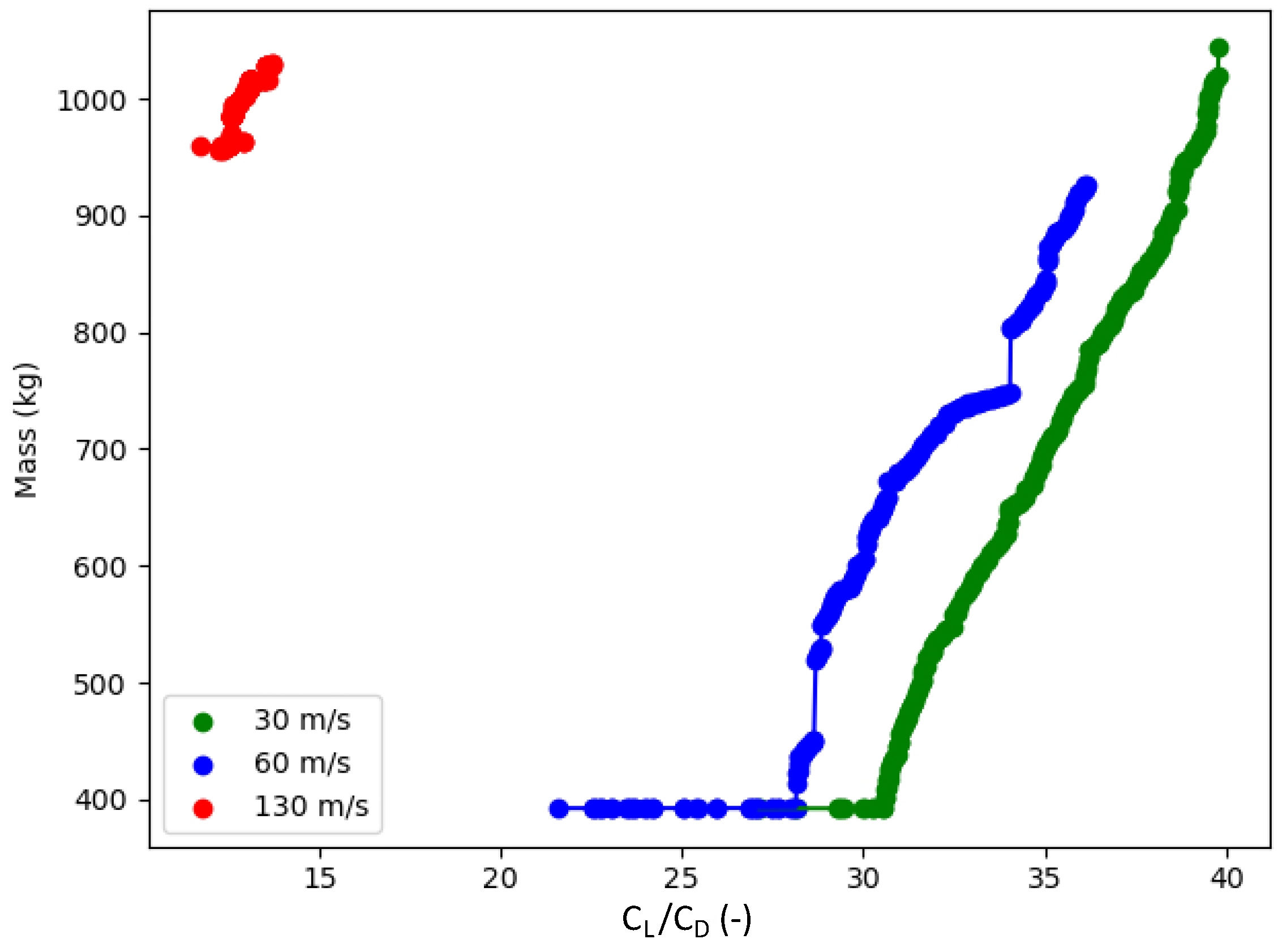
The plot presented in Figure 8 delineates the Pareto fronts for the three analyzed cruise speeds, 30 m/s, 60 m/s, and 130 m/s, derived using the same optimization parameters. It is important to note that the results at 130 m/s represent only the feasible solutions. As the cruise speed increases, the Pareto front tends to be narrower and shift toward lower $C_L/C_D$ values, as expected. The results at 130 m/s present an evident distinction. Unlike the relatively distributed Pareto fronts at 30 m/s and 60 m/s, the solutions at 130 m/s are remarkably more clustered. This localized concentration indicates that, at this higher cruise speed, design solutions that avoid flutter are limited, especially within the limits of our design space. Moreover, these solutions at 130 m/s are characterized by relatively high masses and moderate $C_L/C_D$ values. At higher speeds, the overly stringent constraint of flutter speed within our design space leads to results in which, to avoid flutter, the wing structure needs to be heavier, consequently compromising its aerodynamic efficiency.

4. Concluding Remarks

An SBO methodology for designing wings considering both performance and aeroelasticity constraints was successfully implemented using four different open-source Python codes. This methodology uses Extra Tree Regressors to mitigate the computational cost associated with this wing design problem, and it was tested to solve a multi-objective optimization problem considering three cruise speeds.

Although the surrogate models exhibited suitable performance, certain discrepancies appear, especially in drag coefficient predictions and flutter speed, attributed to observed aeroelastic nonlinearities. Nevertheless, the adopted surrogate models, despite the challenges faced, yielded acceptable results, with errors generally lower than 10%.

To improve the accuracy of the surrogate models in the three cases analyzed, the original design space was revised for each of these cases individually. After this treatment, the optimized designs that maximize $C_L/C_D$ and minimize mass while keeping flutter outside the prescribed boundary presented differences under 5% compared to the corresponding SHARPy simulations. Although this refinement process improved results, it also increased the computational time substantially.

Since the goal was to efficiently integrate aeroelastic analysis, the computational gains were also significant. Direct simulations with SHARPy take about 93.49 s each, while surrogate models offer predictions in under 0.01 s. In terms of optimization, the following observations are made:

• Optimization with 50 generations and 180 population averages 321.76 s, totaling 9000 evaluations. Direct SHARPy simulations would take nearly 10 days.
• A scenario with 200 generations and 280 population takes around 1825.03 s, equaling 56,000 evaluations. Using SHARPy would mean approximately 60 days.

These results highlight the substantial computational time savings when using surrogate models, particularly in optimization scenarios requiring multiple evaluations.

References

1. Afonso, F.; Vale, J.; Oliveira, É.; Lau, F.; Suleman, A. A review on non-linear aeroelasticity of high aspect-ratio wings. Prog. Aerosp. Sci. 2017, 89, 40–57. [Google Scholar] [CrossRef]
2. Jonsson, E.; Riso, C.; Lupp, C.A.; Cesnik, C.E.; Martins, J.R.; Epureanu, B.I. Flutter and post-flutter constraints in aircraft design optimization. Prog. Aerosp. Sci. 2019, 109, 100537. [Google Scholar] [CrossRef]
3. Peherstorfer, B.; Willcox, K.; Gunzburger, M. Survey of Multifidelity Methods in Uncertainty Propagation, Inference, and Optimization. Siam Rev. 2018, 60, 550–591. [Google Scholar] [CrossRef]
4. Giselle Fernández-Gonino, M.; Park, C.; Kim, N.H.; Haftka, R.T. Issues in Deciding Whether to Use Multifidelity Surrogates. AIAA J. 2019, 57, 2039–2054. [Google Scholar] [CrossRef]
5. Yondo, R.; Andrés, E.; Valero, E. A review on design of experiments and surrogate models in aircraft real-time and many-query aerodynamic analyses. Prog. Aerosp. Sci. 2018, 96, 23–61. [Google Scholar] [CrossRef]
6. Li, J.; Du, X.; Martins, J.R. Machine learning in aerodynamic shape optimization. Prog. Aerosp. Sci. 2022, 134, 100849. [Google Scholar] [CrossRef]
7. Mendonça, G.; Afonso, F.; Lau, F. Model order reduction in aerodynamics: Review and applications. Proc. Inst. Mech. Eng. Part G J. Aerosp. Eng. 2019, 233, 5816–5836. [Google Scholar] [CrossRef]
8. Riso, C.; Cesnik, C.E.S. Impact of Low-Order Modeling on Aeroelastic Predictions for Very Flexible Wings. J. Aircr. 2023, 60, 662–687. [Google Scholar] [CrossRef]
9. Gray, A.C.; Riso, C.; Jonsson, E.; Martins, J.R.R.A.; Cesnik, C.E.S. High-Fidelity Aerostructural Optimization with a Geometrically Nonlinear Flutter Constraint. AIAA J. 2023, 61, 2430–2443. [Google Scholar] [CrossRef]
10. Jonsson, E.; Riso, C.; Monteiro, B.B.; Gray, A.C.; Martins, J.R.R.A.; Cesnik, C.E.S. High-Fidelity Gradient-Based Wing Structural Optimization Including Geometrically Nonlinear Flutter Constraint. AIAA J. 2023, 61, 3045–3061. [Google Scholar] [CrossRef]
11. Bryson, D.; Rumpfkeil, M.; Durscher, R. Framework for Multifidelity Aeroelastic Vehicle Design Optimization. In Proceedings of the 18th AIAA/ISSMO Multidisciplinary Analysis and Optimization Conference, Denver, CO, USA, 5–9 June 2017. [Google Scholar] [CrossRef]
12. Thelen, A.S.; Bryson, D.E.; Stanford, B.K.; Beran, P.S. Multi-Fidelity Gradient-Based Optimization for High-Dimensional Aeroelastic Configurations. Algorithms 2022, 15, 131. [Google Scholar] [CrossRef]
13. Lucia, D.J.; Beran, P.S.; Silva, W.A. Reduced-order modeling: New approaches for computational physics. Prog. Aerosp. Sci. 2004, 40, 51–117. [Google Scholar] [CrossRef]
14. Missoum, S.; Dribusch, C.; Beran, P. Reliability-Based Design Optimization of Nonlinear Aeroelasticity Problems. J. Aircr. 2010, 47, 992–998. [Google Scholar] [CrossRef]
15. Stanford, B.; Beran, P. Computational strategies for reliability-based structural optimization of aeroelastic limit cycle oscillations. Struct. Multidiscip. Optim. 2012, 45, 83–99. [Google Scholar] [CrossRef]
16. Shukla, H.; Patil, M. Nonlinear state feedback control design to eliminate subcritical limit cycle oscillations in aeroelastic systems. Struct. Multidiscip. Optim. 2017, 88, 1599–1614. [Google Scholar] [CrossRef]
17. Sohst, M.; Lobo do Vale, J.; Afonso, F.; Suleman, A. Optimization and comparison of strut-braced and high aspect ratio wing aircraft configurations including flutter analysis with geometric non-linearities. Aerosp. Sci. Technol. 2022, 124, 107531. [Google Scholar] [CrossRef]
18. Cea, A.; Palacios, R. Parametric Reduced Order Models for the Aeroelastic Design of Flexible Vehicles. In Proceedings of the AIAA SCITECH 2022 Forum, San Diego, CA, USA, 3–7 January 2022. [Google Scholar] [CrossRef]
19. Toffol, F.; Ricci, S. Preliminary Aero-Elastic Optimization of a Twin-Aisle Long-Haul Aircraft with Increased Aspect Ratio. Aerospace 2023, 10, 374. [Google Scholar] [CrossRef]
20. Sabater, C.; Stürmer, P.; Bekemeyer, P. Fast Predictions of Aircraft Aerodynamics Using Deep-Learning Techniques. AIAA J. 2022, 60, 5249–5261. [Google Scholar] [CrossRef]
21. Goland, M. The Flutter of a Uniorm Cantilever Wing. J. Appl. Mech. 1945, 12, 197–208. [Google Scholar] [CrossRef]
22. Carre, A.; Muñoz, A.; Goizueta, N.; Palacios, R. SHARPy: A dynamic aeroelastic simulation toolbox for very flexible aircraft and wind turbines. J. Open Source Softw. 2019, 4, 1885. [Google Scholar] [CrossRef]
23. Katz, J.; Plotkin, A. Low-Speed Aerodynamics; Cambridge Aerospace Series; Cambridge University Press: Cambridge, UK, 2001. [Google Scholar]
24. Géradin, M.; Cardona, A. Flexible Multibody Dynamics: A Finite Element Approach; John Wiley: Hoboken, NJ, USA, 2001. [Google Scholar]
25. Maraniello, S.; Palacios, R. State-Space Realizations and Internal Balancing in Potential-Flow Aerodynamics with Arbitrary Kinematics. AIAA J. 2019, 57, 2308–2321. [Google Scholar] [CrossRef]
26. Corke, T. Design of Aircraft; Pearson Education, Inc.: Upper Saddle River, NJ, USA, 2003. [Google Scholar]
27. Düssler, S.; Goizueta, N.; Muñoz-Simón, A.; Palacios, R. Modelling and Numerical Enhancements on a UVLM for Nonlinear Aeroelastic Simulation. In Proceedings of the AIAA SCITECH 2022 Forum, San Diego, CA, USA, 3–7 January 2022. [Google Scholar] [CrossRef]
28. Düssler, S.; Palacios, R. Enhanced Unsteady Vortex Lattice Aerodynamics for Nonlinear Flexible Aircraft Dynamic Simulation. AIAA J. 2024, 62, 1179–1194. [Google Scholar] [CrossRef]
29. Wright, J.; Cooper, J. Introduction to Aircraft Aeroelasticity and Loads; Aerospace Series; Wiley: Chichester, UK, 2015. [Google Scholar]
30. Baudin, M.; Christopoulou, M.; Collette, Y.; Martinez, J.M.; Lee, A.D.; Sjögren, R.; Svensson, D. pyDOE2: An Experimental Design Package for Python. 2020. Available online: https://pythonhosted.org/pyDOE/# (accessed on 31 October 2023).
31. Pedregosa, F.; Varoquaux, G.; Gramfort, A.; Michel, V.; Thirion, B.; Grisel, O.; Blondel, M.; Prettenhofer, P.; Weiss, R.; Dubourg, V.; et al. Scikit-learn: Machine Learning in Python. J. Mach. Learn. Res. 2011, 12, 2825–2830. [Google Scholar]
32. Greenhill, S.; Rana, S.; Gupta, S.; Vellanki, P.; Venkatesh, S. Bayesian Optimization for Adaptive Experimental Design: A Review. IEEE Access 2020, 8, 13937–13948. [Google Scholar] [CrossRef]
33. Cardoso, I.; Dubreuil, S.; Bartoli, N.; Gogu, C.; Salaün, M. Constrained efficient global multidisciplinary design optimization using adaptive disciplinary surrogate enrichment. Struct. Multidiscip. Optim. 2024, 67, 23. [Google Scholar] [CrossRef]
34. Geurts, P.; Ernst, D.; Wehenkel, L. Extremely randomized trees. Mach. Learn. 2006, 63, 3–42. [Google Scholar] [CrossRef]
35. Federal Aviation Administration. Office of Primary Responsibility ACE-100, Small Airplane Directorate. In System Safety Analysis and Assessment for Part 23 Airplanes; Technical Report 23.1309-1E; Federal Aviation Administration: Washington, DC, USA, 2011. [Google Scholar]
36. Deb, K.; Pratap, A.; Agarwal, S.; Meyarivan, T. A fast and elitist multiobjective genetic algorithm: NSGA-II. IEEE Trans. Evol. Comput. 2002, 6, 182–197. [Google Scholar] [CrossRef]
37. Biscani, F.; Izzo, D. A parallel global multiobjective framework for optimization: Pagmo. J. Open Source Softw. 2020, 5, 2338. [Google Scholar] [CrossRef]
Figure 1. Implemented surrogate-based optimization methodology.
Applsci 14 02384 g001
Figure 2. Visual comparison of the results obtained using the SHARPy simulations (in blue) and the surrogate model (in orange) in the testing phase of the SMs.
Applsci 14 02384 g002
Figure 3. Learning curves of flutter velocity model.
Applsci 14 02384 g003
Figure 4. Distribution of optimization solutions along design variable boundaries for both objectives: C L / C D maximization (above, in green) and mass minimization (below, in red). Units of mass are given in kg.
Applsci 14 02384 g004
Figure 5. Pareto fronts for Case 1 (cruise speed of 30 m/s).
Applsci 14 02384 g005
Figure 6. Pareto fronts for Case 2 (cruise speed of 60 m/s).
Applsci 14 02384 g006
Figure 7. Pareto fronts for Case 3 (cruise speed of 130 m/s).
Applsci 14 02384 g007
Figure 8. Pareto fronts across analyzed cruise speeds.
Applsci 14 02384 g008