Comparison of Unsteady Low- and Mid-Fidelity Propeller Aerodynamic Methods for Whirl Flutter Applications

Abstract

Aircraft configurations with propellers have been drawing more attention in recent times, partly due to new propulsion concepts based on hydrogen fuel cells and electric motors. These configurations are prone to whirl flutter, which is an aeroelastic instability affecting airframes with elastically supported propellers. It commonly needs to be mitigated already during the design phase of such configurations, requiring, among other things, unsteady aerodynamic transfer functions for the propeller. However, no comprehensive assessment of unsteady propeller aerodynamics for aeroelastic analysis is available in the literature. This paper provides a detailed comparison of nine different low- to mid-fidelity aerodynamic methods, demonstrating their impact on linear, unsteady aerodynamics, as well as whirl flutter stability prediction. Quasi-steady and unsteady methods for blade lift with or without coupling to blade element momentum theory are evaluated and compared to mid-fidelity potential flow solvers (UPM and DUST) and classical, derivative-based methods. Time-domain identification of frequency-domain transfer functions for the unsteady propeller hub loads is used to compare the different methods. Predictions of the minimum required pylon stiffness for stability show good agreement among the mid-fidelity methods. The differences in the stability predictions for the low-fidelity methods are higher. Most methods studied yield a more unstable system than classical, derivative-based whirl flutter analysis, indicating that the use of more sophisticated aerodynamic modeling techniques might be required for accurate whirl flutter prediction.

1. Introduction

Whirl flutter, as an aeroelastic instability, affects the design of aircraft configurations with elastically supported propellers or rotors [1,2]. Turboprop aircraft represent one category where the prevention of whirl flutter can require trade-offs in the design of, e.g., engine suspension. Reducing cabin vibrations demands low stiffness in the engine support for better dynamic isolation, while aeroelastic stability requires high support stiffness [3]. To enable the design and certification of the next generation of propeller aircraft, accurate simulation-based whirl flutter predictions integrated into the frequency-domain flutter analysis workflows for propeller-driven aircraft are necessary.

For example, a classical, simplified rigid propeller–pylon system is shown in Figure 1a, where the propeller is located at distance a from the pylon (pivoting point). The propeller is flexibly mounted on the pylon to allow for rotations of the propeller about the pitch ($\theta$) and yaw ($\psi$) axes. Two corresponding rotary springs with stiffness values, $K_{\theta }$ and $K_{\psi }$, are used to model the elastic properties of the pylon, along with the respective inertia, which also represents the inertia of the engine. Linearized around the zero angle of attack, the physical displacement of the propeller hub ($\Delta {\underline{x}}_{hub}$) can be determined using the modal matrix of the non-rotating system ($\underline{\mathsf{\Phi }}$) and the vector of generalized coordinates $\underline{q}$.

$$\underset{\Delta {\underline{x}}_{hub}}{\underbrace{\left(\begin{array}{c}y\\ z\\ \theta \\ \psi \end{array}\right)}}=\underset{\underline{\mathsf{\Phi }}}{\underbrace{\left\{\begin{array}{cc}0& a\\ -a& 0\\ 1& 0\\ 0& 1\end{array}\right\}}}\underset{\underline{q}}{\underbrace{\left(\begin{array}{c}\theta \\ \psi \end{array}\right)}}$$

(1)

Whirl flutter predictions can be displayed as stability maps (see Figure 1b). The line indicates the stability boundary, which separates regions of stable and unstable combinations of pivot stiffness. This boundary is obtained by varying the pivot stiffness in pitch and yaw and evaluating the aeroelastic stability at a fixed operating point. Instead of the stiffness values, the uncoupled pitch and yaw frequencies are used. Consequently, the boundary shows the uncoupled frequencies in pitch and yaw required for neutral stability (i.e., undamped aeroelastic response). The curve can be generally divided into two branches. The main branch is a parabola with an axis of symmetry on the 45° line. Points below the parabola represent whirl flutter, while points outside the parabola indicate a stable behavior. It can be seen from Figure 1b that the most critical point is represented by equal frequency in pitch and yaw. A boundary with a larger extent (i.e., the curve is shifted in the $\Delta {\omega }_{stab}$ direction) indicates a less stable system, since higher stiffness is required to obtain neutral stability. The branches parallel to the axes represent the divergence boundaries. The described approach is a simplified version of the design problem for turboprop engine mounts [3] and used throughout this work for presenting whirl flutter results.

Currently, rigid propeller blade aerodynamic derivatives are often used within the flutter assessment of turboprop aircraft [4]. This method was developed by Houbolt and Reed [5] in the early 1960s after the accidents with the Lockheed Electra [6]. The derivatives describe the linearized aerodynamic load response of a rigid propeller about its hub when perturbed, e.g., by a disc pitch or yaw angle. Ribner [7] previously described a method to derive the derivatives relevant for aircraft flight mechanics. Ribner’s and Houbolt and Reed’s methods were compared to experimental results [8], and the Houbolt/Reed method was found to be conservative. Later, in 1989, Rodden and Rose [9] demonstrated the inclusion of such derivatives (based on the Houbolt/Reed method) into flutter analysis using MSC Nastran, paving the way for its inclusion into the flutter assessment of full propeller aircraft configurations. Since then, the method has found application in certification [4], design and optimization [10,11], as well as parameter studies [12,13,14], due to its computational efficiency.

Despite being fast and robust, the method by Houbolt and Reed makes some assumptions: It neglects blade elasticity, as well as aerodynamic interaction with the wing, and simplifies the unsteady aerodynamics of the propeller. The stabilizing influence of blade elasticity was recently discussed by one of the authors [15] and is not be detailed in this work. Aerodynamic interaction between the propeller and the wing is often neglected in the literature, although Rodden and Rose [9] suggested an approach to couple the Houbolt/Reed method with wing aerodynamics modeled with the doublet lattice method (DLM). The effect of aerodynamic interaction was shown to be slightly destabilizing in some cases [10], depending on the modes and frequencies involved. The last assumption concerns the aerodynamic modeling of the propeller. The Houbolt/Reed method is based on a quasi-steady, linearized strip theory approach, using Theodorsen’s function for unsteady correction [5]. The steady state (and thus the thrust and torque) is neglected, and no wake model is considered for the induced velocities.

While this work mainly focuses on propeller whirl flutter, there are parallels with respect to the so-called 1P hub loads in terms of aerodynamic phenomena and solution methods. These are the steady in-plane loads a propeller experiences under non-axial inflow. The thesis by Smith [16] summarizes some low-fidelity methods to predict them, while Fei et al. [17] compare mid- and high-fidelity approaches to the prediction of propeller aerodynamics under (even high) angles of attack. CFD-predictions of 1P hub loads have also been compared to wind-tunnel experiments with high-speed propellers [18,19], finding, e.g., significant contributions of the spinner to propeller in-plane forces [18]. The authors also compare different numerical modeling approaches like unsteady time simulation and actuator disc predictions [19]. The literature concerning 1P hub load prediction only covers steady loads, while whirl flutter prediction requires unsteady aerodynamic loads.

Although the Houbolt/Reed method is the most common method used for propeller whirl flutter prediction, other methods can be found in the literature. Hoover and Shen [20,21] used nonlinear airfoil polars coupled with dynamic inflow models under trimmed conditions to study the whirl flutter stability of NASAs X-57 aircraft. They used time-domain methods embedded in rotorcraft comprehensive codes or multi-body simulation to include these more complex aerodynamic methods. Time-domain stability analysis is also commonly applied for tiltrotor aircraft, where the whirl flutter stability of the large, flexible rotors is of major importance [2]. Different studies [22,23] demonstrated the application of mid-fidelity aerodynamic methods in tiltrotor whirl flutter analysis. For example, Corle et al. [23] compared uniform inflow, dynamic inflow and vortex particle method (VPM) results, finding good agreement for the tiltrotor case studied for isolated whirl flutter results. Still, the results cannot easily be transferred to propeller whirl flutter analysis due to the differences in rotor design, operational ranges and the analysis methods used.

As an alternative to time-domain stability analysis, Wang and Chen [24] presented an identification procedure to derive rigid propeller aerodynamic derivates from unsteady vortex lattice method (UVLM) simulations using quasi-steady perturbation of the propeller disc pitch. This approach is compatible with frequency-domain flutter analysis and yields derivatives with fewer assumptions, although it still follows the quasi-steady assumption by Houbolt and Reed. Gennaretti and Greco [25] showed an unsteady, finite-state reduced-order model (ROM) identification method for unsteady aerodynamics of proprotors and applied it for a comparison of low- and mid-fidelity aerodynamic methods. They studied the influence of blade aspect ratio and advance ratio and compared quasi-steady and unsteady airfoil theory with results from a 3D boundary element solver. Their findings indicate that for high advance ratios and blade aspect ratios, the airfoil-based approach yields an under-prediction of the instability ranges. However, their ROM method is not easily transferable to other aerodynamic codes due to its level of integration into the solver.

To the authors’ knowledge, no studies exist in the literature comparing low- and mid-fidelity aerodynamic solution methods with the legacy Houbolt/Reed method for whirl flutter [5] in a framework fully compatible with frequency-domain flutter analysis.

Koch [26] suggested a method to include arbitrary time-domain models of isolated rotors into frequency-domain flutter analysis by identifying frequency-domain transfer matrices about the propeller hub using time-domain perturbations. This method (called transfer matrix or TM-method) allows for the inclusion of different aeroelastic rotor models into whirl flutter analysis, enabling the use of the wide range of tools and methods available for time-domain aeroelastic rotor modeling. It was developed based on an approach to construct helicopter rotor ROMs [27]. The TM-method is applied in this work to study the effect of aerodynamic modeling on the prediction of propeller whirl flutter, giving insights into the underlying mechanism found in unsteady propeller aerodynamics and the reasons for the differences in stability predictions observed.

In the first part of this paper, the aerodynamic methods, including the legacy Houbolt/Reed method, are described and compared. Afterwards, the TM-method, and the workflow and models used are outlined. The results of the studies are presented at the end, finishing with a discussion and outlook.

2. Materials and Methods

This section gives detailed information about the methods used in this work. It starts with a description of the legacy Houbolt/Reed method, which is used as a reference in this paper. Afterwards, the aerodynamic methods are listed and compared, followed by a workflow description of the TM-method, which is used for deriving unsteady aerodynamic characteristics, as well as whirl flutter stability results. Finally, the models and operating points being studied are briefly summarized.

To put this into context, Equation (2) describes the generalized (whirl) flutter problem in the Laplace domain, with s being the Laplace variable.

$$s^2{\underline{M}}_{gen}\underline{q}+s({\underline{D}}_{gen}+{\underline{G}}_{gen})\underline{q}+{\underline{K}}_{gen}\underline{q}={\underline{\mathsf{\Phi }}}^T\underline{f}$$

(2)

The left-hand side of the equation represents the structural airframe with inertia (${\underline{M}}_{gen}$), damping (${\underline{D}}_{gen}$) and stiffness (${\underline{K}}_{gen}$) contributions in generalized coordinates $\underline{q}$. Additionally, the gyroscopic effect induced by the rotation of the propeller is included (${\underline{G}}_{gen}$). The right-hand side describes the unsteady, motion-induced generalized loads. Here, $\underline{f}$ describes the unsteady aerodynamic propeller force and moment vector at the propeller hub (see Equation (3) and Figure 1), which needs to be pre-multiplied by modal matrix $\underline{\mathsf{\Phi }}$ to form the generalized loads.

$$\underline{f}=\left(\begin{array}{c}{F}_y\\ F_z\\ M_y\\ M_z\end{array}\right)$$

(3)

The aerodynamic loads are usually described with transfer functions from propeller hub motion to hub loads [26]. Different descriptions exist in the literature, and the most commonly used one is the formulation using rigid aerodynamic derivatives developed by Houbolt and Reed. The eigenvalues of Equation (2) can be used to assess the stability of the propeller–pylon system. This is often conducted in the frequency domain instead of the Laplace domain (with $i\omega$ replacing s in Equation (2)) [26].

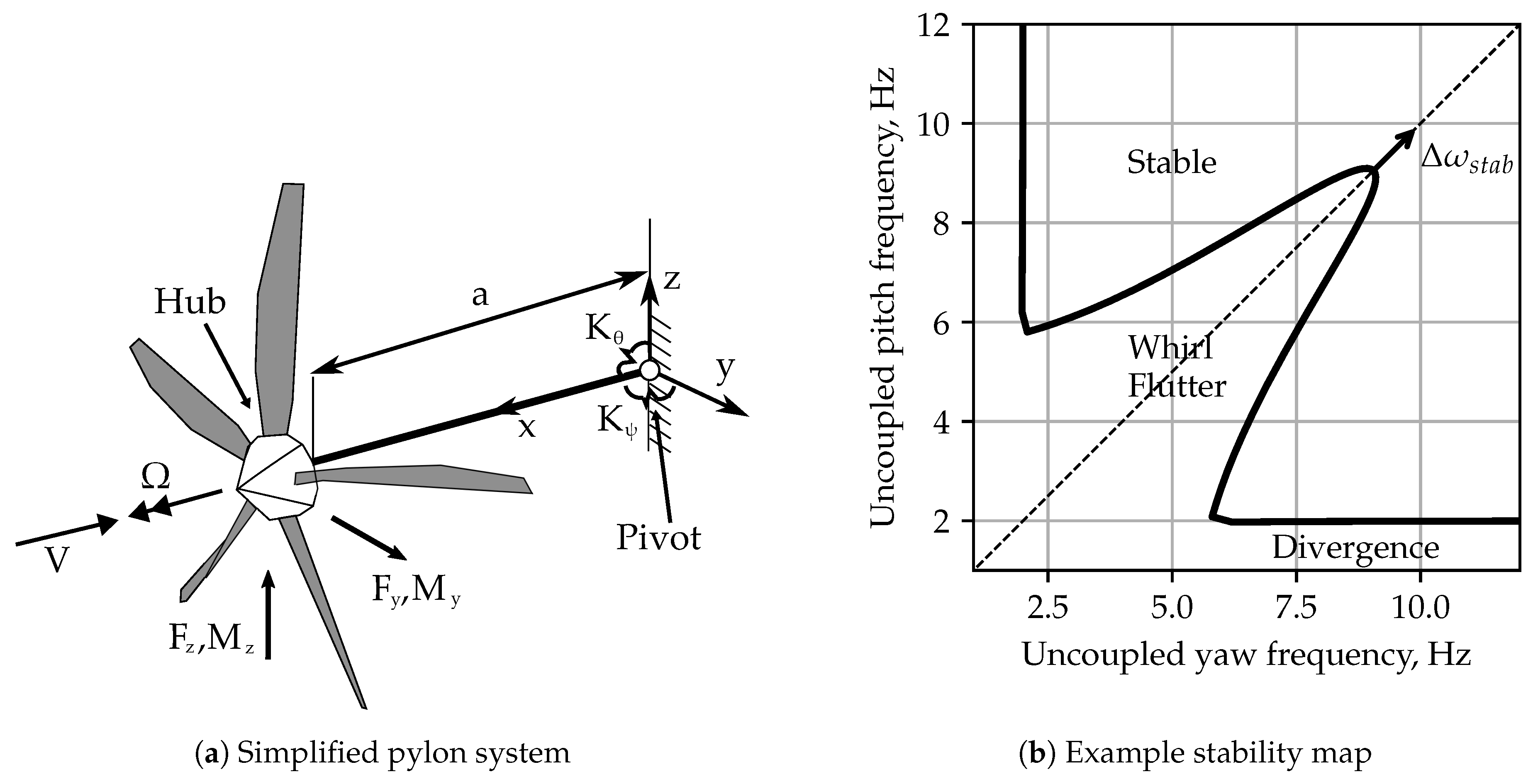
2.1. Houbolt/Reed Method

Houbolt and Reed’s theory [5] represents a pioneering effort in the field of whirl flutter prediction methods in conjunction with an analytical description of unsteady propeller aerodynamics. According to Houbolt and Reed, load vector $\underline{f}$ in Equation (2) can be defined as

$${\underline{f}}_{HR}=\frac{\rho }{2}{V}^{2}2\pi R^3\left[{\underline{K}}_{Aero}(V,\mathsf{\Omega })+s{\underline{D}}_{Aero}(V,\mathsf{\Omega })\right]\Delta {\underline{x}}_{hub}$$

(4)

where $\rho ,V,\mathsf{\Omega }$ and R are the air density and velocity, the rotational speed and the radius of the propeller, respectively. Central to their approach is the formulation of unsteady propeller derivatives. These define the aerodynamic stiffness and damping matrices (${\underline{K}}_{Aero}$ and ${\underline{D}}_{Aero}$) (see Equations (5) and (6)).

$${\underline{K}}_{Aero}(V,\mathsf{\Omega })=\left\{\begin{array}{cccc}0& 0& \frac{C_{y\theta }}{2R}& \frac{C_{y\psi }}{2R}\\ 0& 0& \frac{C_{z\theta }}{2R}& \frac{C_{z\psi }}{2R}\\ 0& 0& C_{m\theta }& C_{m\psi }\\ 0& 0& C_{n\theta }& C_{n\psi }\end{array}\right\}$$

(5)

$${\underline{D}}_{Aero}(V,\mathsf{\Omega })=\left\{\begin{array}{cccc}-\frac{C_{y\psi }}{2RV}& \frac{C_{y\theta }}{2RV}& \frac{C_{yq}}{2V}& \frac{C_{yr}}{2V}\\ -\frac{C_{z\psi }}{2RV}& \frac{C_{z\theta }}{2RV}& \frac{C_{zq}}{2V}& \frac{C_{zr}}{2V}\\ -\frac{C_{m\psi }}{V}& \frac{C_{m\theta }}{V}& \frac{C_{mq}R}{V}& \frac{C_{mr}R}{V}\\ -\frac{C_{n\psi }}{V}& \frac{C_{n\theta }}{V}& \frac{C_{nq}R}{V}& \frac{C_{nr}R}{V}\end{array}\right\}$$

(6)

The derivatives describe the forces and moments on the propeller plane due to the corresponding displacements and velocities of the propeller hub ($\Delta {\underline{x}}_{hub}$) (see Equation (1)). Each of the derivatives corresponds to the change in a load (first index) in response to a perturbation (second index). As an example, $C_{m\theta }$ denotes the change in moment $M_y$ at the propeller hub due to a displacement in pitch $\theta$. Note that according to Houbolt and Reed’s notation for the derivatives, y and z stand for the forces in $F_y$ and $F_z$, while m and n represent the moments in $M_y$ and $M_z$. q and r denote rotational velocities $\dot{\theta }$ and $\dot{\psi }$. Although stiffness properties are a function of translations and rotations, Equation (5) only contains derivatives with respect to rotations $\theta$ and $\psi$. Translatory displacements do not add a perturbation to the propeller disc, so that the first two columns in Equation (5) are zero. In contrast, Equation (6) contains derivatives with respect to rotations (first two columns) and rotational velocities (last two columns). The derivatives in response to $\dot{y}$ and $\dot{z}$ in the first two columns of Equation (6) are described in terms of $\theta$ and $\psi$ rather than $\dot{y}$ and $\dot{z}$ because they linearly depend on the generalized coordinates (refer to Equation (1)). Generally speaking, due to the quasi-steady assumption, a velocity in y or z can be interpreted as a steady induced flow angle. In summary, a total of 16 derivatives are defined, although the inherent symmetry of the model reduces the number of unique derivatives to 8 (e.g., $C_{z\theta }=-C_{y\psi }$) [9]. These derivatives are calculated using blade integrals. Exemplary for $C_{m\theta }$, the equation reads [9]

$$C_{m\theta }=-\left(\frac{N_b}{4}\right)\left(\frac{1}{\pi R}\right){\int }_{{\eta }_0}^1\frac{{\eta }^{2}c\left(\eta \right)C_{l\alpha }\left(\eta \right)G\left(k\right)}{\sqrt{{\left(\frac{J}{\pi }\right)}^2+{\eta }^2}}\frac{A_R}{\left[2+A_R\sqrt{1-M{a}^2(1+{\eta }^2{\left(\frac{\pi }{J}\right)}^2)}\right]}d\eta$$

(7)

with

$$J=\frac{V\pi }{\mathsf{\Omega }R}$$

(8)

and

$$k=\frac{c}{2R\sqrt{{\left(\frac{J}{\pi }\right)}^2+{\eta }^2}}$$

(9)

As seen in Equation (7), the derivative is determined based on an integration along the blade. Here, $\eta$ describes the normalized radius, while ${\eta }_0$ stands for the hub radius. Airspeed and rotational speed of the propeller are described using the advance ratio (J). A Prandtl–Glauert Mach-number ($Ma$) correction in conjunction with a compressible flow aspect ratio ($A_R$) correction is used (see the last factor in the integral in Equation (7)). Further, for each blade section, three factors are important: the chord (c); the local lift curve slope ($C_{l\alpha }$); and a correction due to the unsteady lift lag implemented by utilizing the complex Theodorsen function $C\left(k\right)=F-iG$, which is dependent on the reduced frequency (k). It is worth noting that according to Houbolt and Reed [5], the reduced frequency for each blade section is only dependent on the rotational speed (i.e., J; refer to Equation (9)) and not on the eigenfrequency of the system, which is usually the case in the definition of k. A correction concerning the number of blades ($N_b$) is provided by Rodden and Rose [9], alongside the correction concerning the lift curve slope referred to above. As already mentioned, steady aerodynamic loading including torque and thrust is neglected within this approach. For more detailed information on blade integrals and corrections, the reader is referred to the original literature [5,9].

To determine the influence of the propeller derivatives on whirl flutter stability, a sensitivity analysis is conducted for the derivatives according to Houbolt and Reed. Each of the eight derivative pairs is varied with a scale factor between 60% and 140% of a baseline value while keeping the other seven pairs equal to the baseline value for a reference configuration. For each combination, flutter analyses are performed with varying pivot stiffness to find the required stiffness for neutral stability. These required stiffness values are then converted into uncoupled frequency. The relative difference from the baseline uncoupled frequency ($\Delta {\omega }_{stab}$) serves as the comparison parameter and is defined as

$$\Delta {\omega }_{stab}=\frac{{\omega }_{stab,i}-{\omega }_{stab,ref}}{{\omega }_{stab,ref}},$$

(10)

A positive value indicates a destabilization, since the boundary is shifted to larger frequencies. It is worth noting that the pitch stiffness and yaw stiffness are kept equal during this sensitivity analysis, as this represents the most critical combination for classical whirl flutter (see Figure 1b).

The results of the sensitivity study are presented in Figure 2. Stabilizing contributions are seen for $C_{y\theta }$, $C_{z\theta }$ and $C_{mq}$. On the other hand, $C_{n\theta }$ has a largely destabilizing effect. Negligible influences are observed for $C_{yq}$, $C_{m\theta }$, $C_{zq}$ and $C_{nq}$. The last two were also often neglected in previous studies due to their comparatively low values [9]. Please note that the same relations hold for the symmetrical partners of the mentioned derivatives (both were varied simultaneously during the sensitivity analysis).

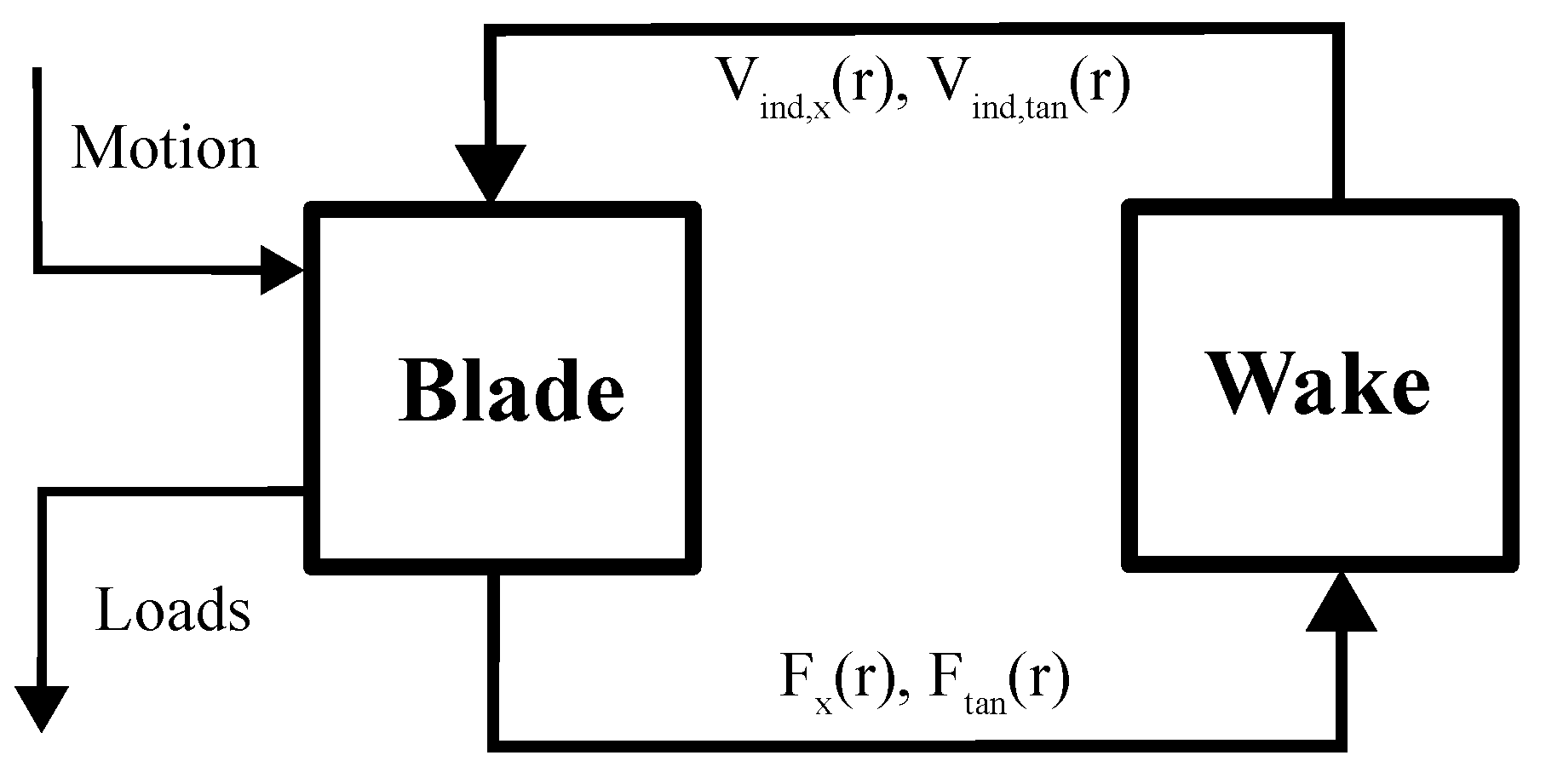
2.2. Aerodynamic Methods

The following section introduces the aerodynamic methods compared in this work. Some assumptions were made to limit the number of studies in this paper and to facilitate the understanding of the causes for potential differences among results. The limitations are listed below, and their potential impact is discussed in the Discussion section:

• No compressibility effects: It is known from the literature that compressibility has a significant impact on whirl flutter stability through the change in the lift curve slope [28]. As most methods compared in this paper are based on potential flow aerodynamics, they neglect compressibility and can only account for it using correction techniques like Prandtl–Glauert correction factors. Despite being available in most codes, this correction is skipped for better comparability.
• Linear airfoil polars: To keep the number of parameters small and to make the comparison among codes easier, linear airfoil polars for a symmetric NACA 0008 airfoil in potential flow are used. This results in a linear lift curve with slope $C_{l\alpha }$. All other contributions, like drag or camber effects, are neglected in this study.
• Limited number of operating conditions: The study is limited to a single operating range, a turboprop propeller in fast forward flight, since operating conditions with high advance ratios are the most relevant for whirl flutter.
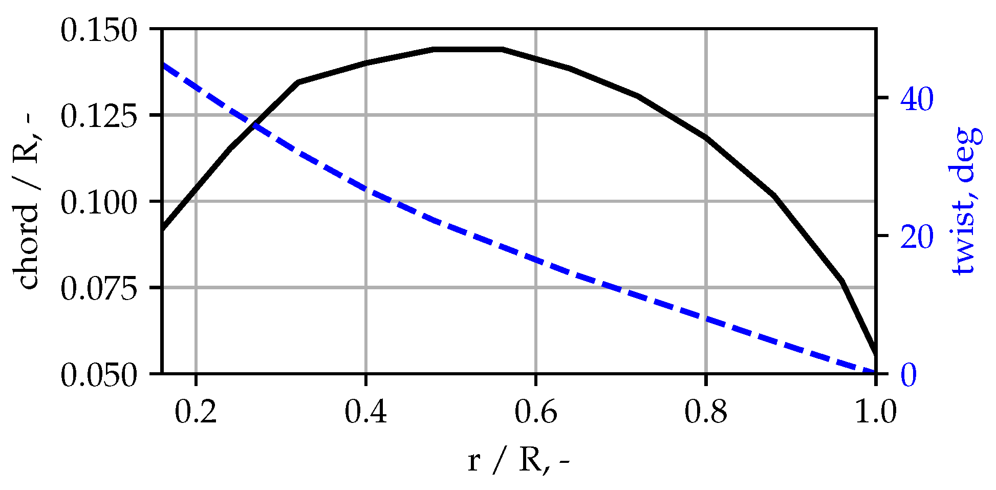
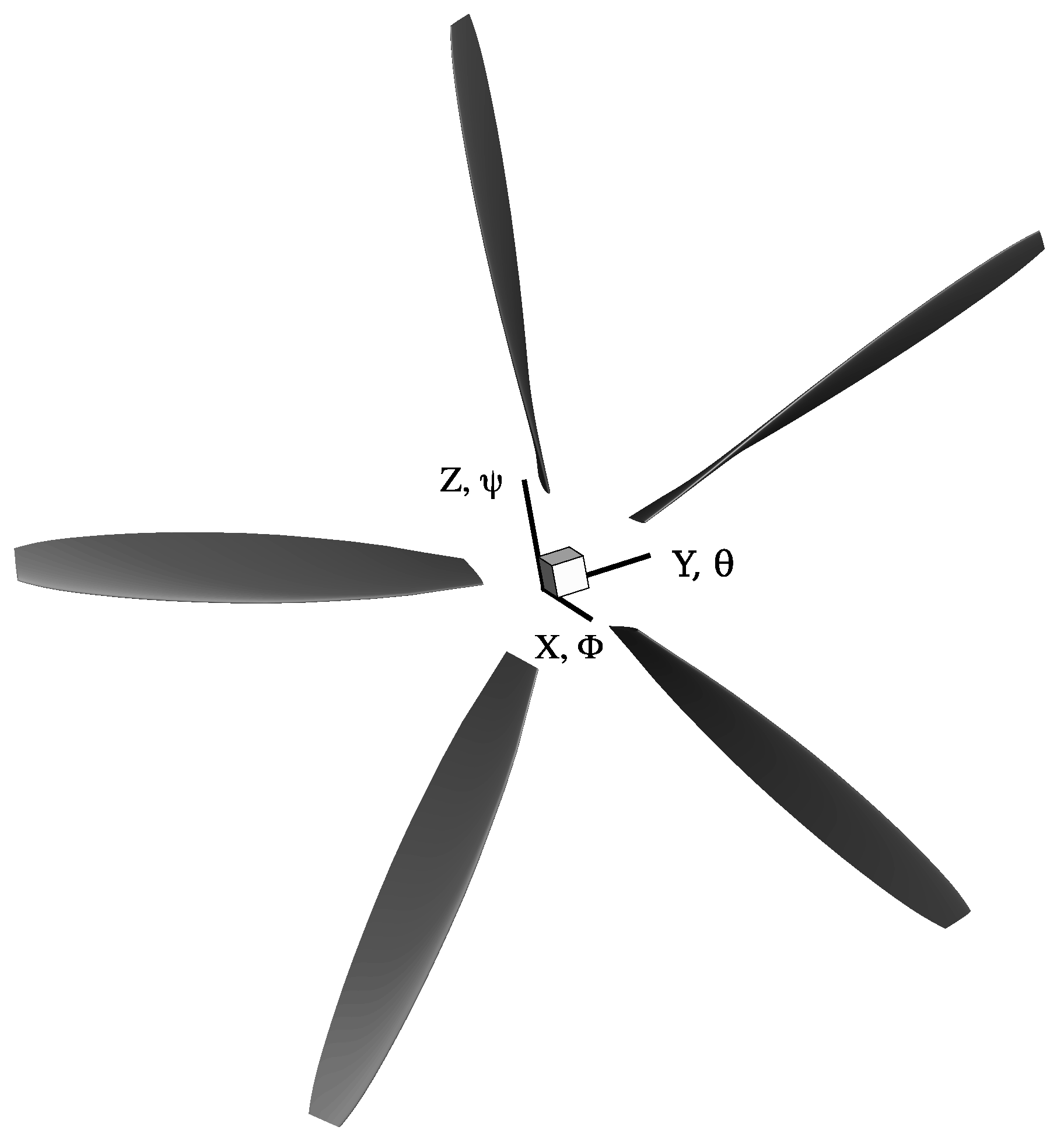
• Only one geometry: Only a generic five-bladed turboprop propeller is used for this study. No variations with respect to the blade aspect ratio, the number of blades or the blade geometry are conducted.
• Only blade aerodynamics: In this work, only the unsteady aerodynamics attributed to the propeller blades are studied. Contributions from the spinner, nacelle or wing are neglected.
• Rigid propeller blades: To perform a comparison with the classical Houbolt/Reed derivatives, the propeller blades are assumed to be rigid. For a study on the influence of elasticity, the reader is referred to the literature (e.g., Koch and Koert [15]).

The different methods compared in this work with respect to unsteady propeller aerodynamics and their impact on whirl flutter stability predictions are listed in

Table 1. Comparison of aerodynamic methods used in this work.

Method	Blade Lift Method	Wake Method	Tip Loss	Comp. Time
UPM [29,30,31]	2D vortex lattice on camber surface + 3D source/sink panels on blade surface	Free panel wake	Included in free wake	Hours
DUST-Panel [32,33]	3D doublet and source panels on blade surface	Free vortex particle wake	Included in free wake	Hours
DUST-UVLM [32,33]	2D vortex lattice on camber surface	Free vortex particle wake	Included in free wake	Hours
DUST-LL [32,33]	1D lifting line using airfoil polars	Free vortex particle wake	Included in free wake	Minutes–Hours
BEM+Wagner	Strip theory using airfoil polars + Wagner’s function for unsteady lift lag [34]	Weighted blade element momentum theory [16,35]	Prandtl–Glauert	Minutes
Wagner	Strip theory using airfoil polars + Wagner’s function for unsteady lift lag [34]	No induced velocity model	No tip loss model	Seconds
Quasi-steady	Strip theory using airfoil polars	No induced velocity model	No tip loss model	Seconds
Houbolt/Reed	Linearized strip theory ($C_{L\alpha }$ only) + Theodorsen’s function for unsteady lift lag	No induced velocity model	Aspect ratio correction	Seconds
Houbolt/Reed quasi-steady	Linearized strip theory ($C_{L\alpha }$ only)	No induced velocity model	Aspect ratio correction	Seconds

. The first column lists the methods and the name/abbreviation used throughout this paper. The following three columns contain a brief description of the relevant features distinguishing the methods from each other, split into the blade lift method, the wake method and the tip loss method. The order of magnitude for computational time is also given in the last column for comparison. The methods (or rows in Table 1, respectively) are split into three categories: The first four methods are categorized as mid-fidelity due to their explicit wake modeling and their ability to capture interference effects. The following three methods are categorized as low-fidelity due to the simplifications in modeling and their short run times. The last two rows represent the Houbolt/Reed method introduced earlier.

In general, all aerodynamic methods used in this paper have to solve the equilibrium between local blade lift distribution and wake strength, as illustrated in Figure 3 for every given motion and time step. The specific implementation of the blade lift or wake formulation and their interaction depends on the method and solution of the coupled system in the tool used.

The mid-fidelity methods used in this paper rely on different types of blade discretization, ranging from a full 3D surface grid using 3D doublets and source panels over 2D vortex lattice formulations to 1D lifting line theory with radial discretization into airfoil sections [32]. The wake models in UPM and DUST, on the other hand, are very similar, using free-wake methods with panel wake [29,30,31] or discrete vortex particle wake [32,33]. Free-wake methods allow for the capturing of the induced velocities of the wake affecting the wake itself and the propeller. Due to this complete description of the wake, no tip loss model is required.

The low-fidelity methods are based on a strip theory approach for blade aerodynamics, using airfoil polars for the primary relationship between angle of attack and lift. To capture the unsteady effect of the near wake, a time-domain formulation for the lift lag effect according to Wagner’s function (see [34] for details) is applied in some methods. The induced velocities of the whole wake due to thrust and torque on the propeller are either neglected or described quasi-steadily using the blade element momentum (BEM) method [35]. Due to the non-axial inflow condition during propeller disc pitch motion, a special formulation of the BEM, the Weighted BEM from [16], is used to cover the azimuthal variation in the induced velocities. Still, in the BEM, no interaction of the radial sections is considered, so a tip loss model using Prandtl–Glauert’s tip (and hub) loss factor is used in the BEM method [35]. A more detailed discussion of the influence of the different BEM-formulations on the results are presented in Appendix C.

The method by Houbolt and Reed was described earlier. The relevant features for the comparison in Table 1 are the linearized form of the strip theory (only taking perturbational lift contributions from $C_{l\alpha }$ into account), the optional correction for lift lag using Theordorsen’s function (see Equation (7)), the lack of a model for the induced velocities and the finite blade span (or tip loss) correction using the blade aspect ratio ($A_R$).

2.3. Transfer Matrix Method

The goal of this work is to compare different aerodynamic methods with special focus on the unsteady aerodynamics and their influence on whirl flutter predictions. Hence, a method is required to derive the relevant unsteady aerodynamic quantities and to conduct whirl flutter stability predictions based on them. This paper employs the transfer matrix (TM) method recently developed by one of the authors [26] to identify the relevant transfer functions based on time-domain simulations. The TM-method is centered around describing the unsteady perturbation response of the propeller hub loads, $\underline{f}$, to hub motion $\Delta {\underline{x}}_{hub}$ in the frequency domain according to a frequency-dependent transfer matrix, ${\underline{H}}_{prop}$:

$${\underline{f}}_{TM}={\underline{H}}_{prop}(i\omega ,V,\mathsf{\Omega },\rho )\Delta {\underline{x}}_{hub}$$

(11)

with

$${\underline{H}}_{prop}(i\omega ,V,\mathsf{\Omega },\rho )=\left\{\begin{array}{cccc}{F}_{yy}& F_{yz}& F_{y\theta }& F_{y\psi }\\ F_{zy}& F_{zz}& F_{z\theta }& F_{z\psi }\\ M_{yy}& M_{yz}& M_{y\theta }& M_{y\psi }\\ M_{zy}& M_{xz}& M_{z\theta }& M_{z\psi }\end{array}\right\}$$

(12)

The transfer matrix captures all features included in the time-domain method, such as unsteady aerodynamics and wake descriptions. It is used to extract aerodynamic transfer functions, similar to Houbolt and Reed’s aerodynamic derivatives but capturing the full frequency dependency of the methods studied. The workflow is described in the following. The steps in italics are not required for the original TM-method workflow but are employed in this work to gain further insights into the unsteady aerodynamic behavior:

• Trimming to a steady operating point in axial flow
  The propeller is trimmed to achieve a target steady thrust coefficient $C_T$ and to bring the system to an equilibrium, around which the perturbations are employed. Trimming is achieved by iteratively changing the blade pitch angle until $C_T$ matches the desired thrust. For each iteration, the system is integrated in time with a fixed blade pitch until a steady state in the hub loads is reached. The resulting equilibrium is saved for further restarts.
• Response of the system to steady disc pitch perturbation (1P hub loads)
  Instead of directly identifying the full, frequency-dependent transfer functions for hub motion perturbations, the quasi-steady response to disc pitch (or disc angle of attack) is identified first. Starting from the equilibrium point in "1.", the disc pitch angle is perturbed by a steady $1^{\circ }$ inclination, and the system is integrated in time until a steady state in the hub loads is achieved over one period.
• Perturbation of the hub motion and recording of the hub load response
  To identify the frequency-dependent transfer matrices, the propeller is perturbed in y-translation and disc pitch $\theta$ using unsteady pulse-shaped excitation (for low-fidelity methods) or harmonic forced motion (for mid-fidelity codes). The response of the hub load components in the time domain is recorded. The system is integrated in time until the transient response has decayed. For harmonic forced motion, this process is repeated for several perturbation frequencies (5 Hz, 10 Hz, 20 Hz) to cover the desired range for the frequency-domain flutter analysis.
• Identification of the frequency-domain transfer function from motion to loads
  By converting both motion and load time histories into the frequency domain using Fourier transformation, the frequency-domain transfer function from hub motion to hub loads can be identified through division. The scalar transfer functions (e.g., disc pitch to moment about the z-axis) are then arranged into the transfer matrices in Equation (12). Due to axial symmetry, the transfer functions for z-translation and disc yaw $\psi$ can be derived from symmetry and do not have to be calculated separately.
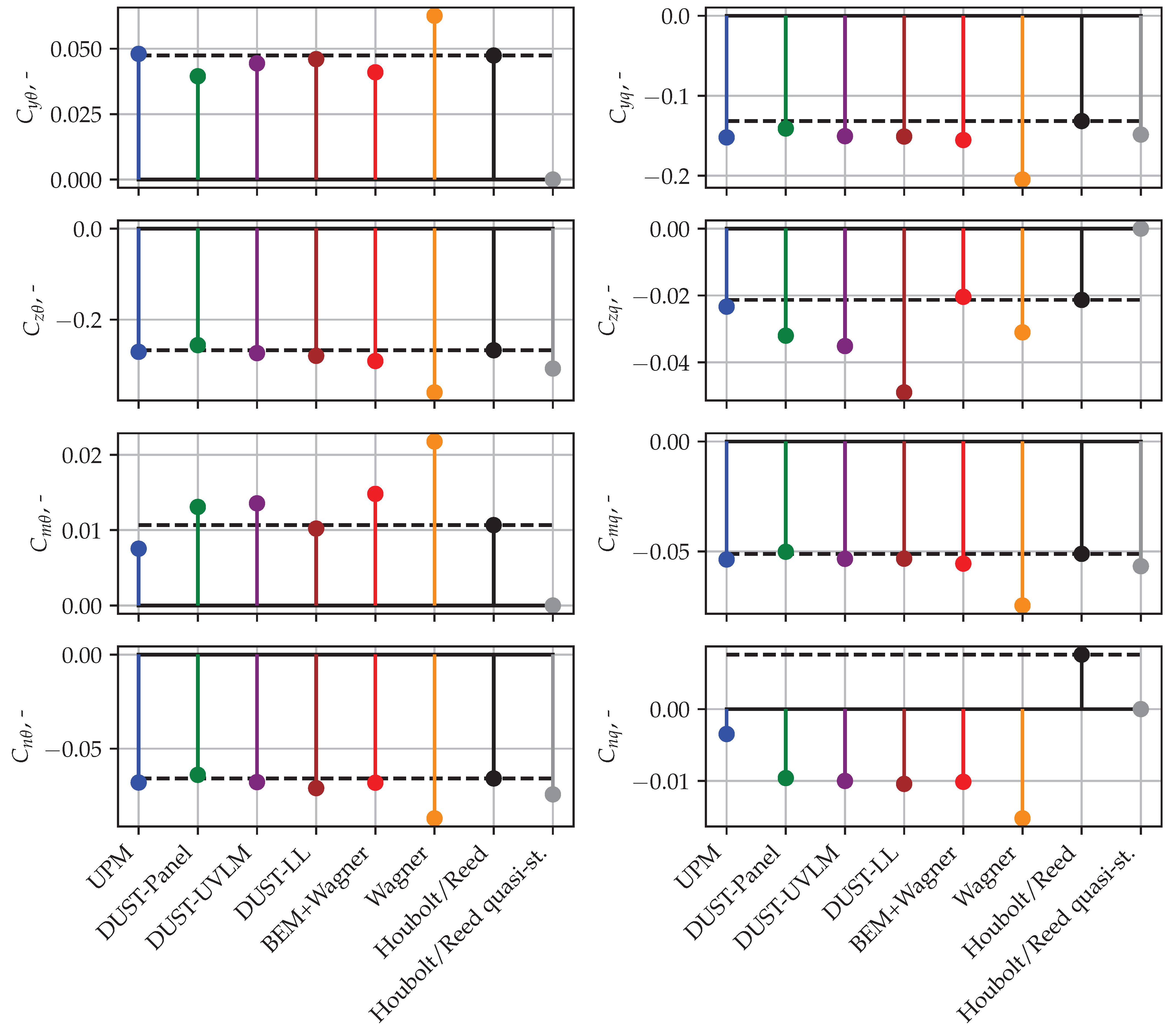
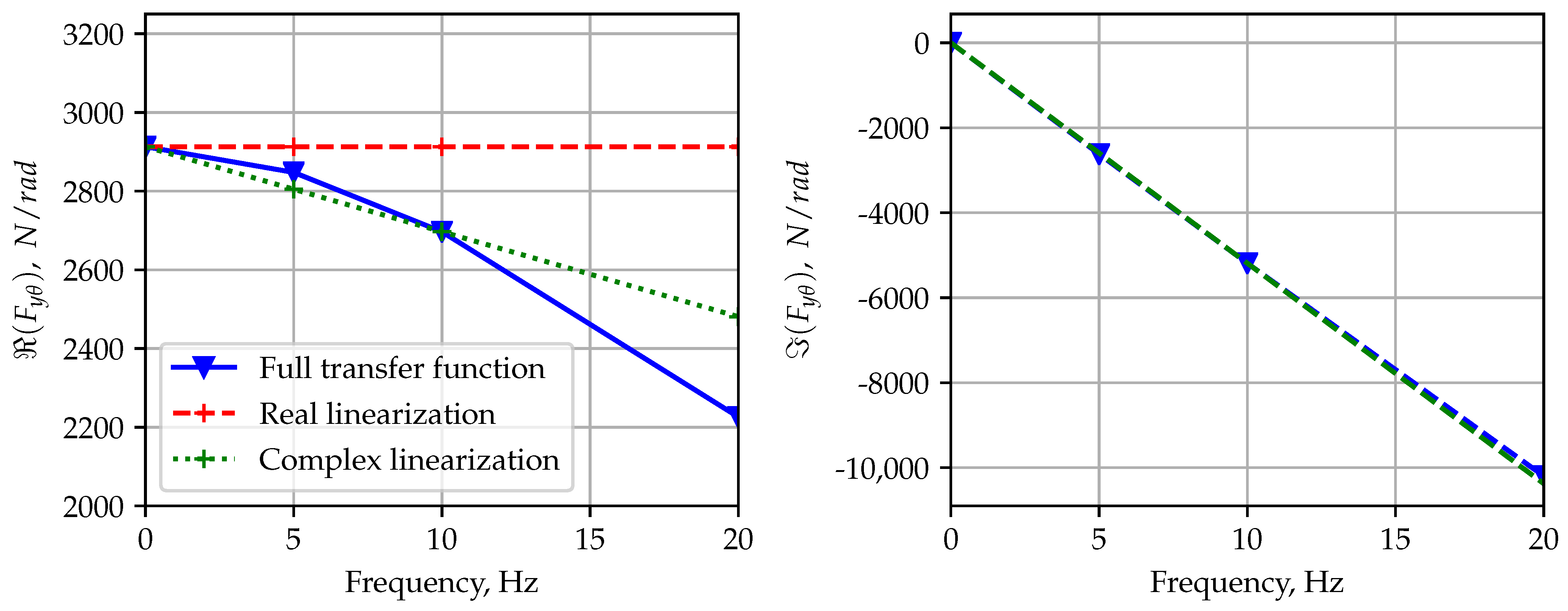
• Linearization with respect to frequencyfor comparison with Houbolt/Reed derivatives
  To compare the frequency-dependent transfer matrices with the propeller derivatives by Houbolt and Reed, the transfer matrices are linearized with respect to frequency. The constant part of the real part is converted into the aerodynamic stiffness, and the linear slope of the imaginary part is used as aerodynamic damping (see Appendix A for more insights into the linearization procedure). By using the same non-dimensionalization as that by Houbolt and Reed, derivatives which can be used for direct comparison are obtained.
• Flutter solution in the frequency domain
  To assess the impact of different aerodynamic methods on whirl flutter predictions, the transfer matrices are inserted into the equation of motion (see Equation (2)) and solved in the frequency domain either using the pk method or pole fitting [26].

The workflow is used for all aerodynamic methods, and results from each step are described and discussed in the second part of the paper.

2.4. Models

The propeller model used in this work resembles a generic propeller blade close to the geometry of an off-the-shelf turboprop propeller. It is a five-bladed propeller with variable blade pitch operated under constant rotational speed. The basic geometry of the blade is shown in Figure 4 by means of chord and twist distribution. The resulting aspect ratio according to [5] is 6.87. The twist is the geometric twist, which is added on top of the blade pitch angle resulting from the trim analysis. All radial sections are positioned to form a straight 50% chord line. A lift curve slope ($C_{l\alpha }$) of 6.5894 is used for all sections (when applicable in the method).

Figure 5 shows the resulting model geometry together with the global coordinate system. The global x-axis points in the direction of flight, while the y- and z-axes span the propeller plane. The global reference frame (to which all loads in this paper are referenced) stays fixed and does not move or tilt with the forced motion.

For the whirl flutter stability analysis, the propeller is coupled to the simplified pylon model shown in Figure 1. The structural properties of the system are listed in

Table 2. Properties of the pylon system about the pivoting point.

Property	Symbol	Value
Pitch/yaw inertia	$I_{\theta }$/$I_{\psi }$	$97.42$  $\mathrm{k}\mathrm{g}$${\mathrm{m}}^2$
Total polar inertia of rotating parts	$I_{\varphi }$	$6.69$  $\mathrm{k}\mathrm{g}$${\mathrm{m}}^2$
Pitch stiffness	$K_{\theta }$	$I_{\theta }\ast {\omega }_{\theta }^2$
Yaw stiffness	$K_{\psi }$	$I_{\psi }\ast {\omega }_{\psi }^2$
Pylon length	a	0.425, 0.85 and 1.7 $\mathrm{m}$

and resemble a typical turboprop engine–pylon combination. The pitch stiffness and yaw stiffness are varied for parameter sweeps and derived from uncoupled (non-rotating) pitch or yaw frequency using the equation given in Table 2. According to this model, the distance between pivot point and the propeller plane (a), therefore, scales the force terms in the transfer matrices in comparison to the moment terms. For a short pylon (small a), the moment terms dominate the generalized propeller loads, while for long pylons, the force terms have a higher impact. Three different pylon lengths are, therefore, considered in this paper (see Table 2), called “short”, “medium” and “long”.

Whirl flutter stability results are compared for three different operating points in this paper, which are listed in

Table 3. Overview of operating points studied in this paper.

Name	Airspeed	Shaft Speed	Advance Ratio	Thrust Coefficient	Air Density
	(V, m s−1)	($\mathbf{\Omega }$, rpm)	(J, -)	(${\mathit{C}}_{\mathit{T}}$, -)	($\mathsf{\rho }$, kg m${}^{-\mathbf{3}}$)
$C_T=0,V=V_D$	142	1600	2.13	0.0	1.225
$C_T=0.1,V=V_D$	142	1600	2.13	0.1	1.225
$C_T=0,V=0.5V_D$	71	1600	1.07	0.0	1.225

. They differ in the trim target (i.e., thrust coefficient ($C_T$)) and the advance ratio (i.e., airspeed (V)).

3. Results

After having described the methods and models, the following section covers the results from the individual steps of the analysis.

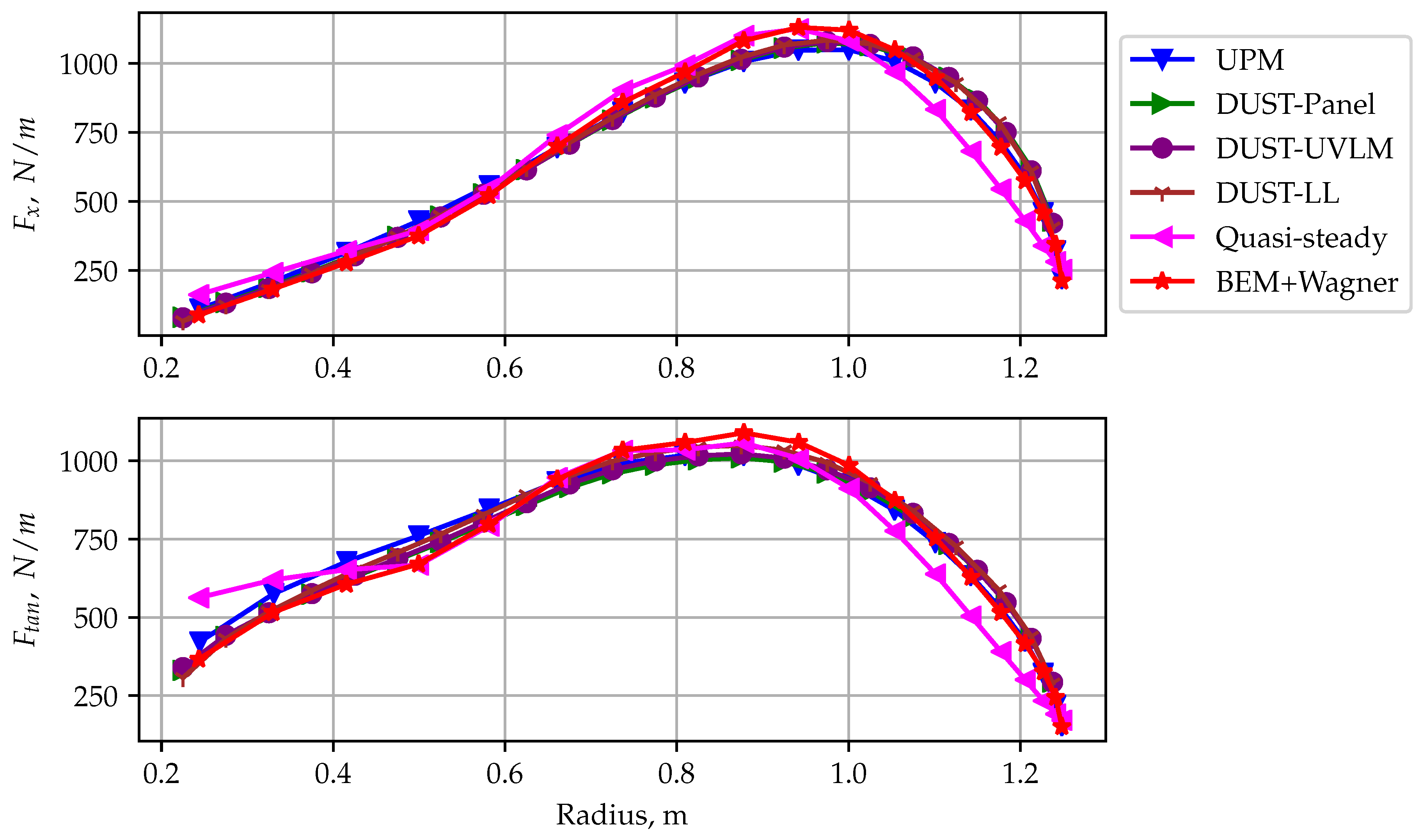
3.1. Comparison of Loads at Axial Inflow

As described in Section 2, the starting point of all simulations is a steady-state condition trimmed on the target thrust by modifying the blade pitch angle. The pitch angles required to match the $C_T=0.1$ trim target are all very close for the methods including wake models (36.4 ± 0.1°), and those without a wake model predict a smaller pitch angle (35.0°). For the no-thrust condition ($C_T=0.$), all methods predict a trim angle of 32.32 ± 0.06°.

Figure 6 shows a comparison of the steady-state axial (or out-of-plane) and tangential (in-plane) load distributions on the blade among the different methods for operating point $C_T=0.1,V=V_D$ from Table 3. Due to the trim condition, the integral on the upper plot is identical for all methods. Overall, the distribution of the steady-state loading over the rotor radius is similar among all methods. The largest differences can be seen for the low-fidelity Quasi-steady method without wake aerodynamics. The lack of induced velocity results in a slight shifting in the load towards the middle of the rotor radius. The BEM+Wagner method also deviates from the mid-fidelity methods, yet the difference is smaller and can be attributed to the (simplified) Prandtl–Glauert tip loss correction. The differences are more pronounced at $C_T$ = 0 but less significant for further analysis, because the load is, in general, very small for this operating point. The Wagner method is not displayed, as it gives the same steady results as the quasi-steady method.

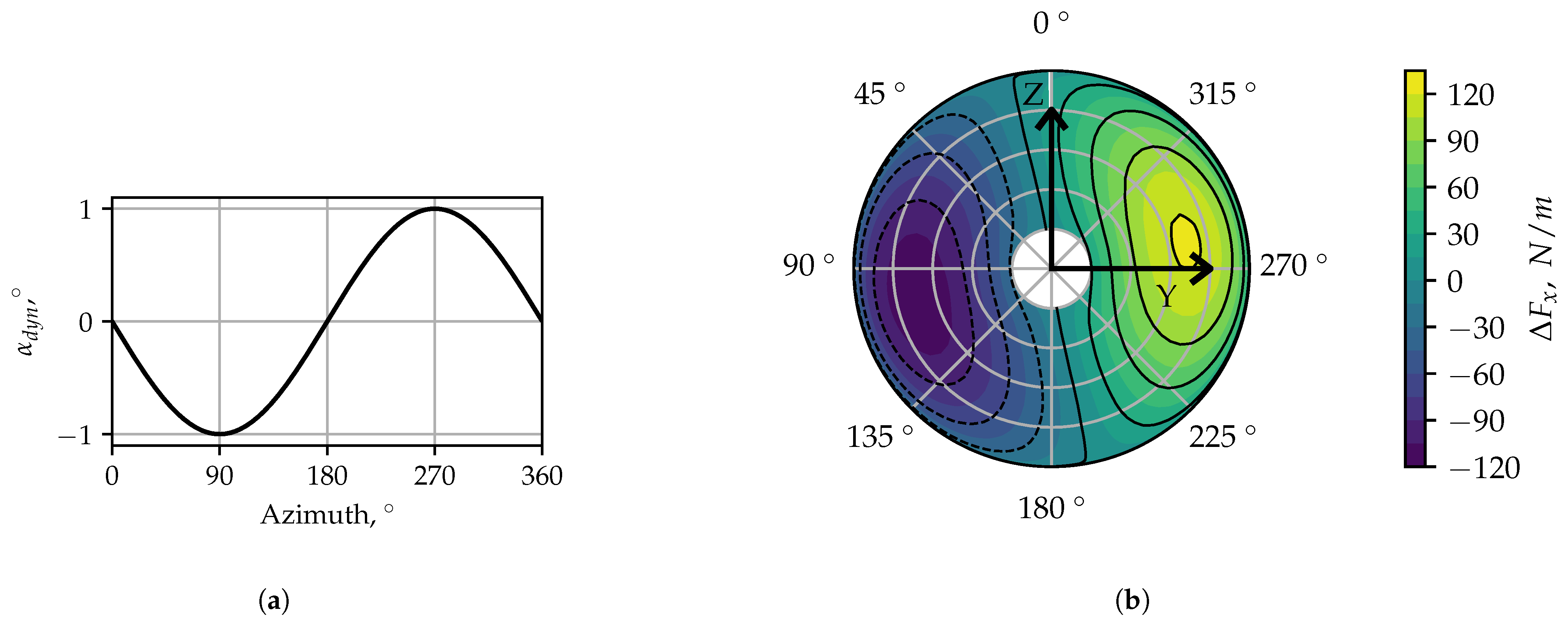
3.2. Loads for Steady Propeller Disc Pitch (1P Hub Loads)

Before progressing to the unsteady results, the response of the propeller models to a steady perturbation of the propeller disc pitch (as induced by an aircraft angle of attack), also called 1P hub loads [16], is discussed. Only small perturbations and thus linearized transfer functions are shown. The name 1P hub loads originates from the once-per-revolution (1P) angle-of-attack variation (see Equation (13) and Figure 7a) that each individual blade experiences during one revolution due to kinematics [11]. The first-harmonic nature of the resulting blade loads is filtered out for the hub loads due to the summation over all blades at the propeller hub, resulting in steady loads in the non-rotating system.

$${\alpha }_{dyn}=-\theta ·sin\left(\mathsf{\Omega }t\right)$$

(13)

Figure 7b shows the resulting out-of-plane blade load distribution over one revolution (in Figure 7b, results from UPM are shown). The propeller disc in this example is tilted around the global y-axis, so the top is tilted forwards. Solid contour lines (on the right side of the disc) indicate an increase in local thrust in these sectors, and dashed contour lines (left side of the disc), a loss in thrust. As Figure 7b shows, the lift for a tilt around the global y-axis is mainly anti-symmetric with respect to the global z-axis, resulting in the coupling torque ($M_{z\theta }$), which is one of the main drivers of whirl flutter instability (see $C_{n\theta }$ in Figure 2). Additionally, it can be observed that the maximum of the unsteady- lift lags in phase behind the angle of attack, which has its maximum and minimum exactly at ${270}^{\circ }$ and ${90}^{\circ }$, respectively (see Equation (13) and Figure 7a). This (and the corresponding lift deficiency) is caused by the unsteady aerodynamic liftlag effects [11]. This unsteadiness leads to a reduction in the amplitude of the 1P hub loads. A further reduction in the lift amplitude can be attributed to effects derived from induced velocity. Sectors with more lift generate more circulation shed in the wake and thus higher induced velocities affecting the disc, reducing the local angle of attack and the resulting lift. A second consequence of the phase lag between angle of attack and lift maximum is the development of a moment about the global y-axis. This can be visualized as a phase shift in the resulting global moment from the z-axis to higher azimuth angles, resulting in an $M_y$ component. This (and the corresponding side force, $F_y$) are called off-axis terms, because they are perpendicular to the primary load response (also called in-phase terms in this paper) along the z-axis. Further explanations for the other hub loads can be found in [11].

Figure 8 compares the linear relation between disc pitch and steady hub in-plane loads for the different methods for operating point $C_T=0,V=V_D$ from Table 3. The top row shows the force transfer functions, and the bottom one, the corresponding moments. The plots on the right side correspond to the in-phase terms, mainly caused by the kinematic angle-of-attack variation in the disc. The plots on the left show the off-axis terms caused by the unsteady lift lag effects.

As apparent from Figure 8, the z-force and -moment are predicted to be much higher than the off-axis terms by all methods. Methods that do not account for unsteady lift lag (quasi-steady time-domain and Houbolt/Reed quasi-st. methods) only predict the in-phase force terms, and the off-axis force term ($F_y$) is zero. The same applies for the off-axis moment term ($M_y$), although the quasi-steady time-domain method predicts a small value due to the airfoil torque arising from the offset between lift reference point at quarter chord and the y-axis, which is neglected in the Houbolt/Reed formulation. In general, the relative variation among the methods is higher for the off-axis terms, as their prediction is based on the unsteady lift model employed and not mainly on the kinematics. The prediction by the mid-fidelity methods (top four rows in each plot) are all within the same range, deviating by only about 5% with respect to each other (for $M_{z\theta }$). Only predictions in $M_{y\theta }$ deviate a bit more, as this component is influenced by the chord-wise distribution of the lift and thus the offset moment between lift vector and y-axis, which is different among the mid-fidelity methods.

For the low-fidelity methods, the quasi-steady time-domain method over-predicts the in-phase loads compared with the mid-fidelity codes (e.g., by 47% in $M_{z\theta }$). This is due to the lack of the lift deficiency (unlike the Wagner method, which over-estimates $M_{z\theta }$ by 28%), as well as induction and tip loss effects (a further difference from BEM+Wagner). Because, additionally, no off-axis terms are predicted, this method is not further used in the following analysis. The equivalent quasi-steady Houbolt/Reed formulation incorporates the aspect ratio correction (see Equation (7)), explaining the better match in amplitude of the z-force and -moment due to the reduction in lift due to tip loss effects. The same applies to the comparison between the unsteady Wagner method and the baseline Houbolt/Reed results, where the differences can also be mainly attributed to the missing tip loss correction in the Wagner method. The baseline Houbolt/Reed results for the 1P hub loads match well with the mid-fidelity predictions, even though the method lacks an aerodynamic wake model. The results from BEM+Wagner (the most detailed low-fidelity method) show good agreement with the mid-fidelity codes, with slight over-predictions of $F_{z\theta }$ and $M_{y\theta }$.

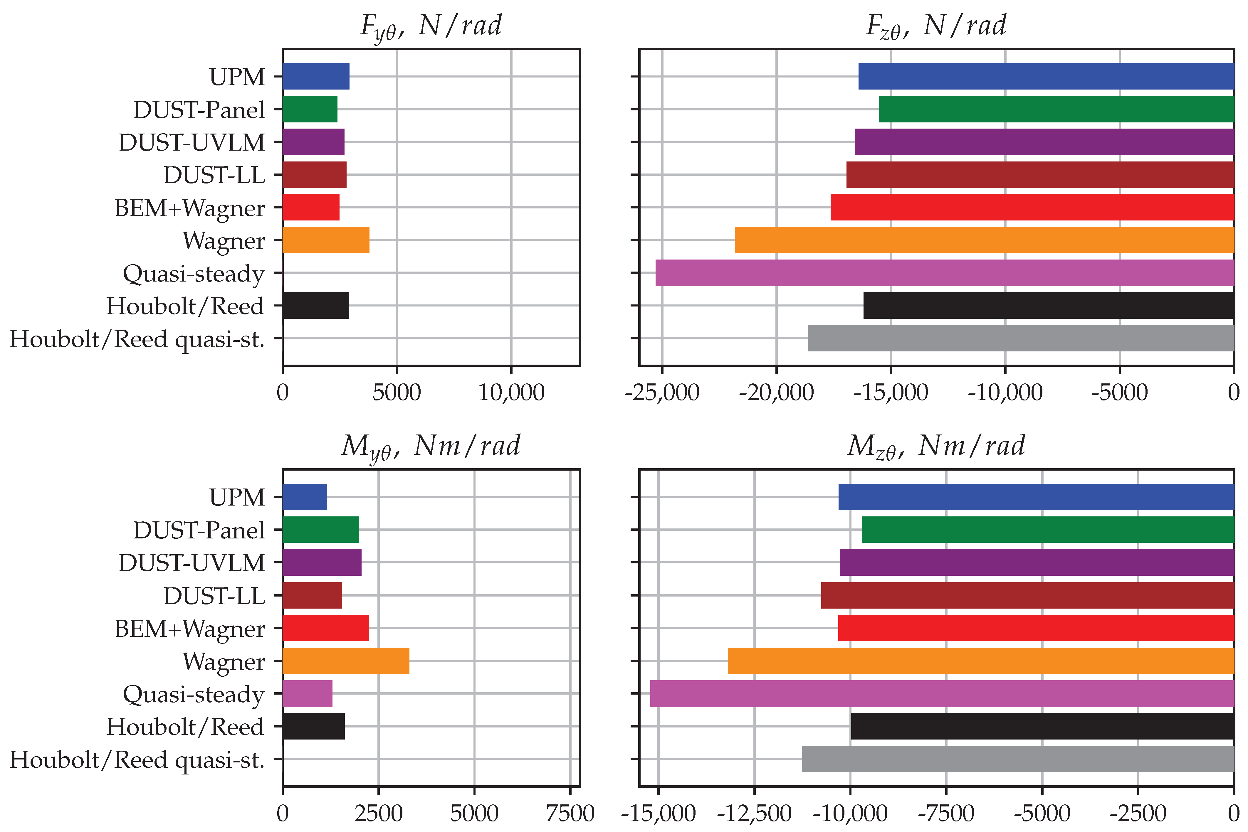
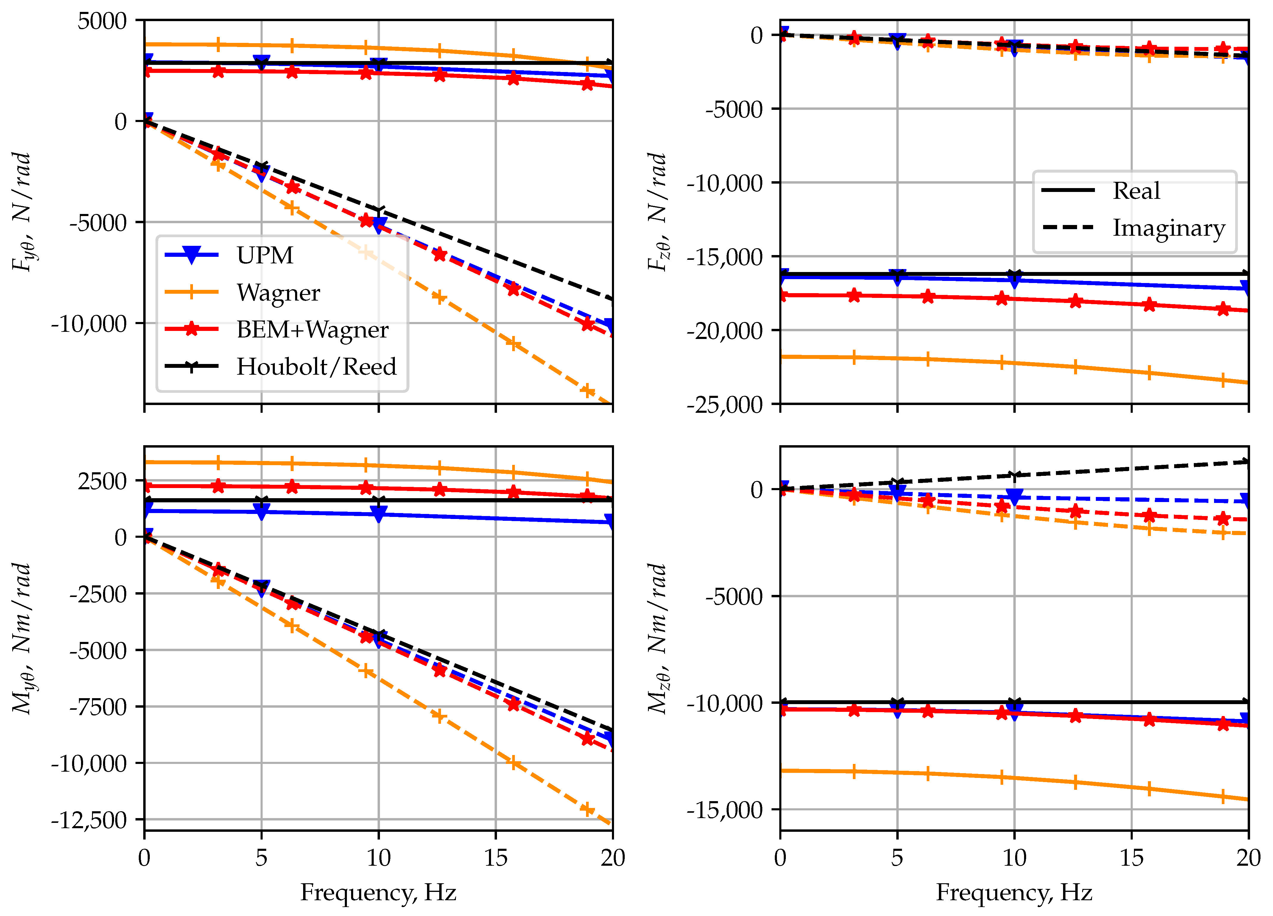
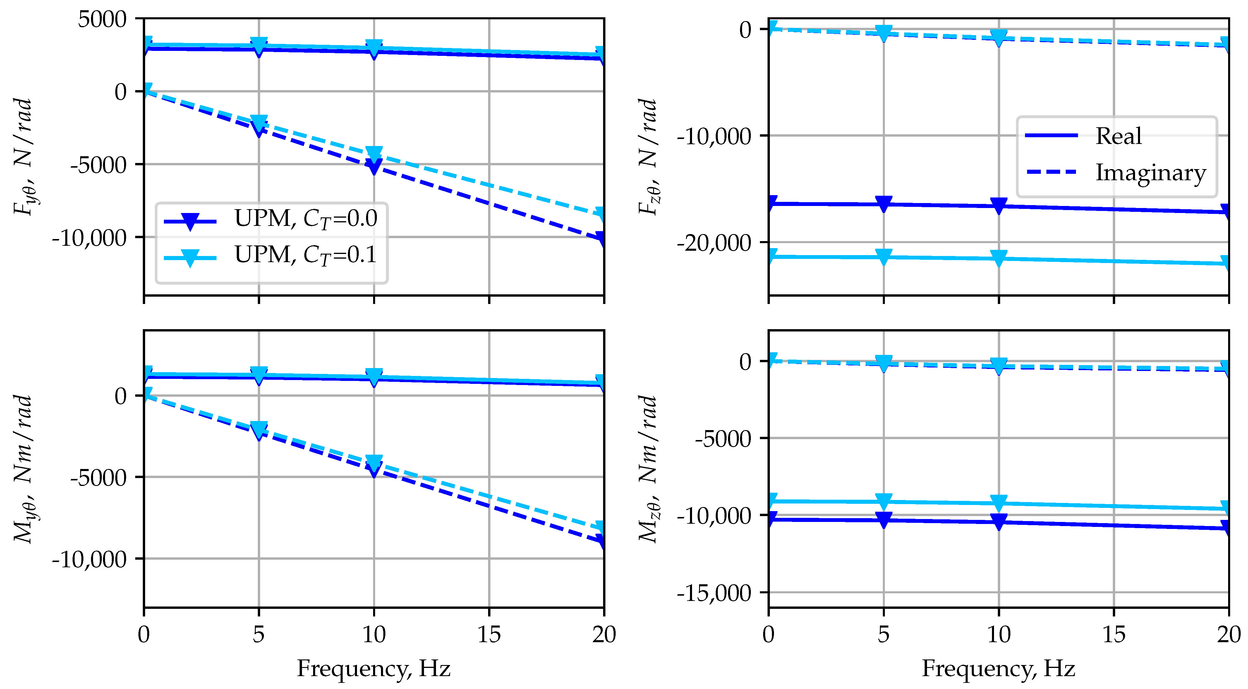
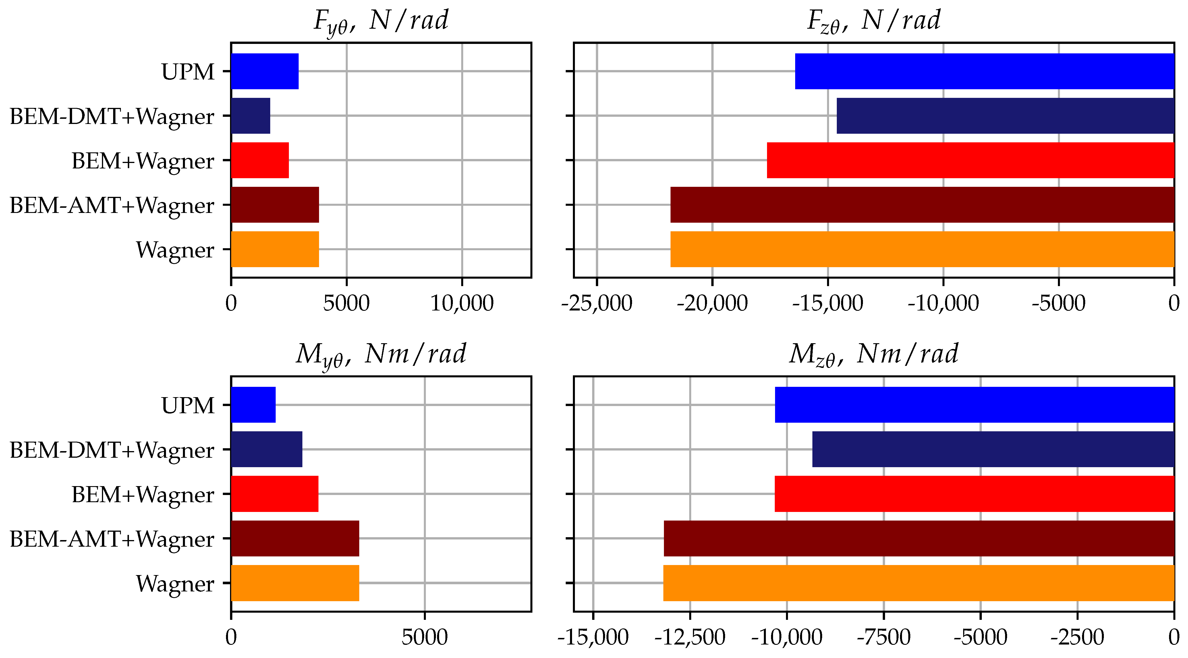
3.3. Loads and Transfer Matrices for Propeller Hub Motion

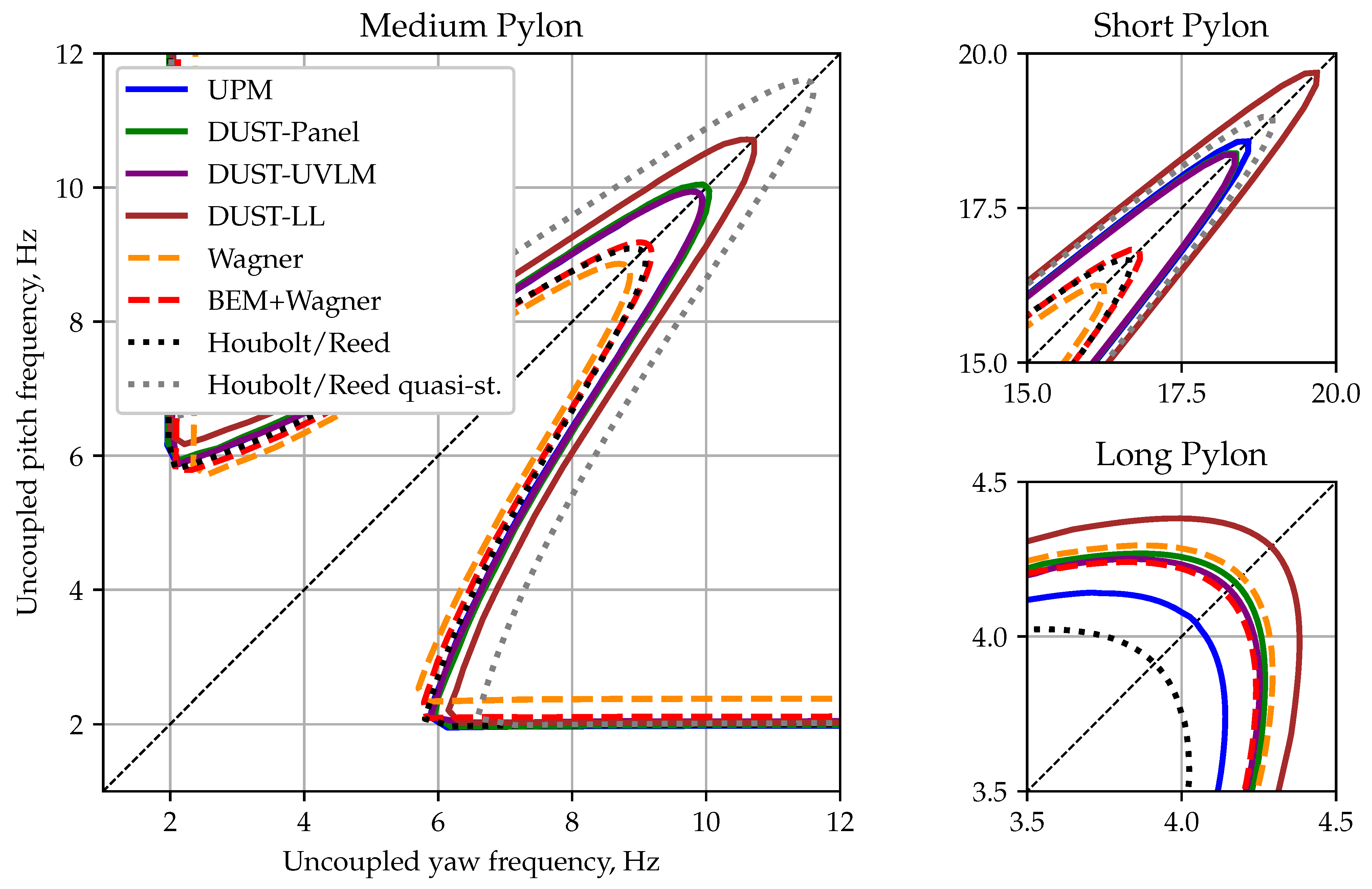
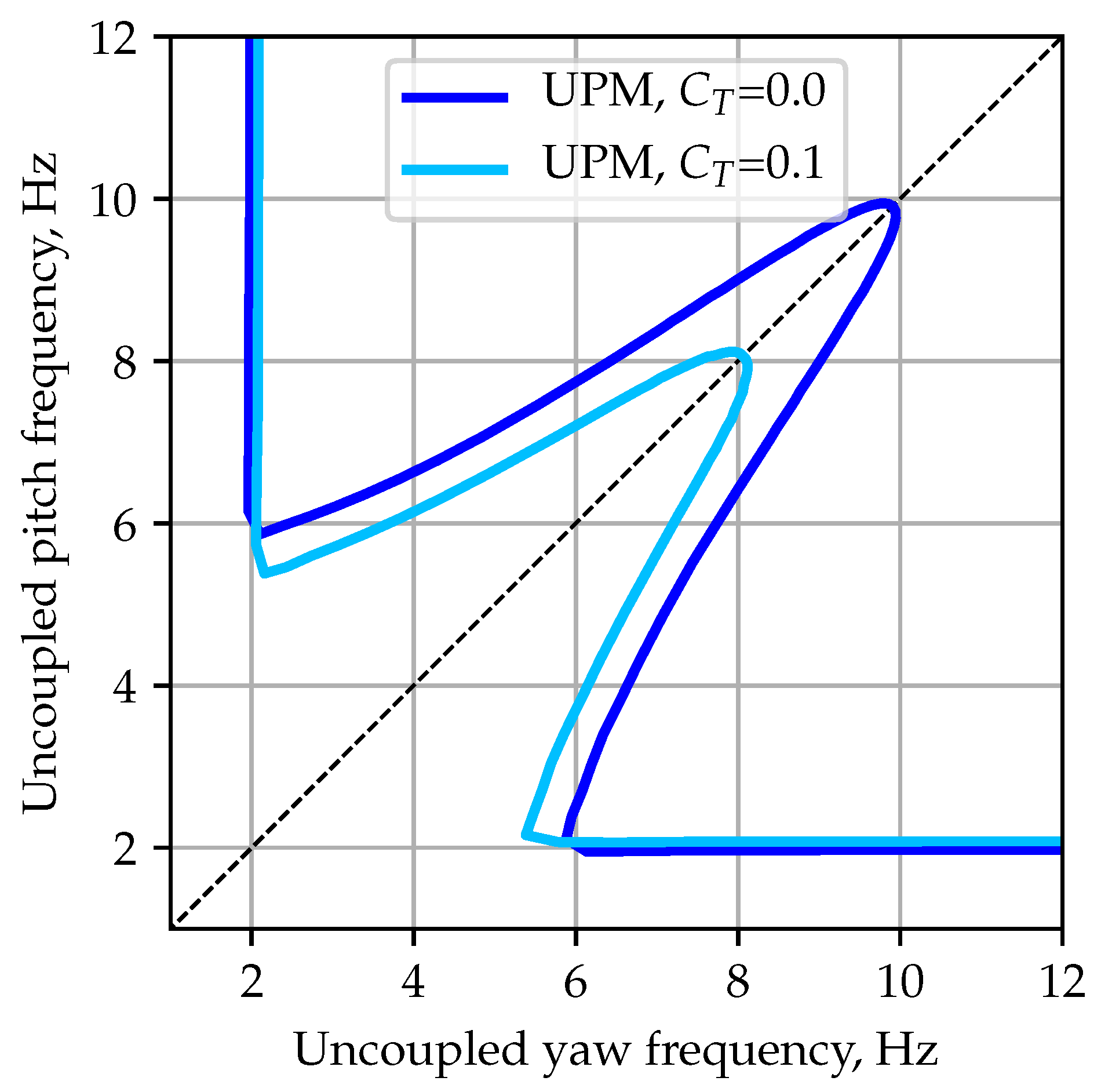
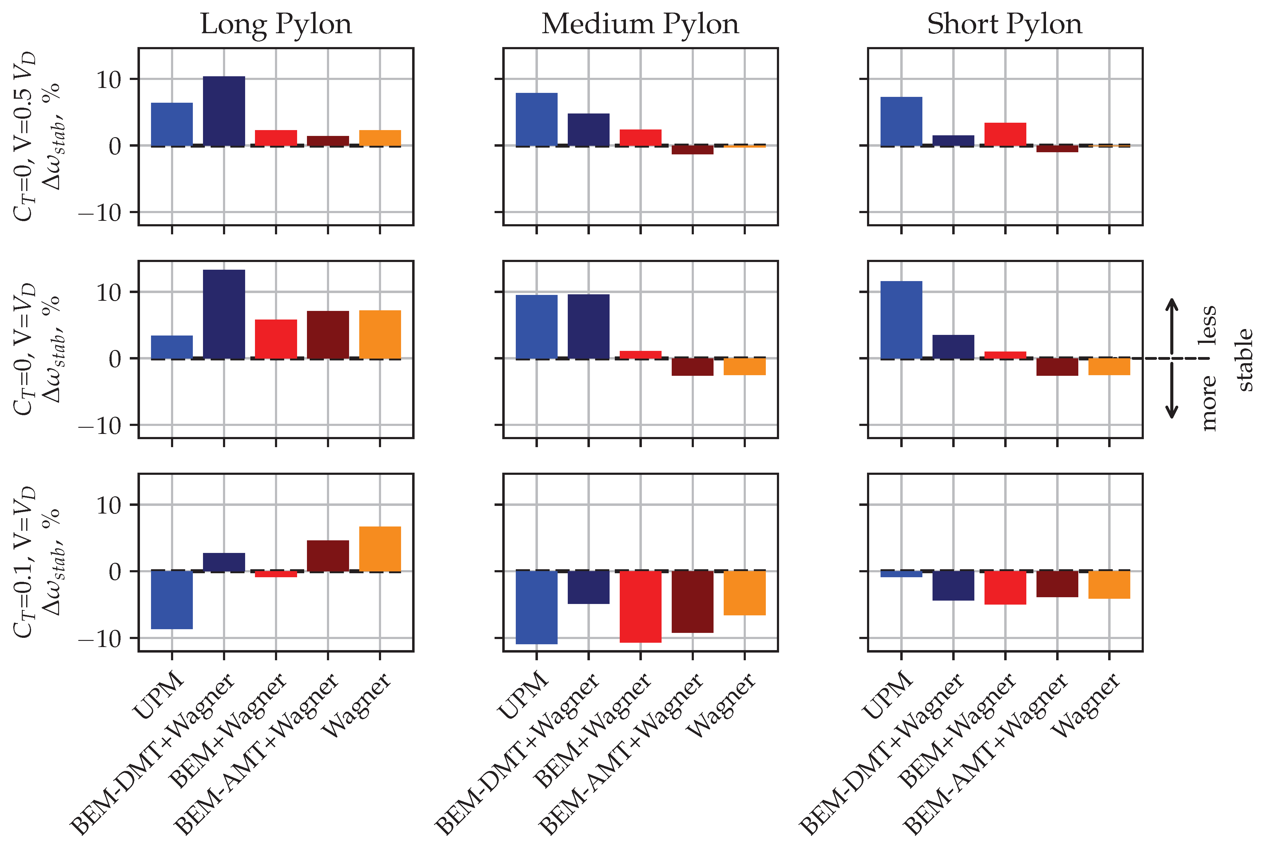
The previous subsection assessed the transfer behavior for zero frequency about the propeller hub. In this subsection, this is extended by showing transfer functions which describe the response to harmonic perturbations about the propeller hub. This subsection mainly focuses on perturbation response with respect to disc pitch $\theta$. Due to axial symmetry, the transfer functions for disc yaw ($\psi$) are equivalent (with some signs being changed). The transfer functions with respect to harmonic disc in-plane (y and z) translation can be derived, as a steady velocity $\dot{z}$ is almost equivalent to a steady disc pitch $\theta$. For the whirl flutter studies shown later, the translation terms are still computed separately, but they are not shown in this subsection for the sake of brevity.

Figure 9 shows these transfer functions for a selection of aerodynamic methods for operating point $C_T=0,V=V_D$ from Table 3. The top row shows the force components, and the bottom row, the hub moments. Each plot contains the real (solid line) and imaginary (dashed line) parts of the complex transfer functions plotted over perturbation frequency. The markers indicate the samples identified with harmonic (for the mid-fidelity methods) or pulse (for the low-fidelity methods) perturbation. Only UPM transfer functions are shown for the mid-fidelity codes for better visibility, representing the other mid-fidelity methods which give similar results. All transfer functions are real-valued for zero frequency and equivalent to the 1P hub loads shown in Figure 8. A constant term in the real part (e.g., in the bottom-left plot for $M_{z\theta }$) over frequency indicates aerodynamic stiffness. A linear slope in the imaginary part (e.g., bottom-left plot for $M_{y\theta }$) indicates aerodynamic damping in this component. All other contributions (e.g., the nonlinear decrease in the real part of $M_{z\theta }$) have their origin in an unsteady aerodynamic behavior which is nonlinear with frequency. From Figure 9, some differences from the Wagner method, which predicts higher amplitudes in the transfer functions, can already be observed. This is consistent with the observations for the 1P hub loads in Figure 8. The other methods match reasonably well.

To obtain a more quantitative comparison of all methods, the transfer functions are linearized with respect to frequency. This allows for a split into the derivative form comprising aerodynamic stiffness and damping, similar to the description of the Houbolt/Reed method in Equations (5) and (6). The linearization is conducted by using the zero-frequency samples (to obtain correct transfer functions at zero frequency) and a sample at a chosen frequency (in this work, at 10 Hz perturbation frequency). The real part of the zero-frequency transfer sample is used as aerodynamic stiffness, and the linear slope in the imaginary part, as aerodynamic damping. The resulting values are non-dimensionalized according to Equation (4) and can then be compared to the derivatives from the Houbolt/Reed method. The resulting linearized transfer functions would look similar to the Houbolt/Reed sample in Figure 9, which are already in linear form. Appendix A gives an example for the linearization procedure.

Figure 10 shows a comparison of the eight unique derivatives obtained from the frequency-dependent transfer functions with the derivatives from the Houbolt/Reed method (marked with horizontal dashed lines in each plot). In general, good agreement is found among most methods for derivatives $C_{yq}$, $C_{z\theta }$, $C_{mq}$ and $C_{n\theta }$. These (similar to the 1P hub loads) are the in-phase components, which are mainly related to kinematics [11]. The Wagner method has the highest deviations from the Houbolt/Reed method and the mid-fidelity codes. The BEM+Wagner method matches again very well with the mid-fidelity methods. Larger differences among the predictions can be observed for the other components ($C_{y\theta }$, $C_{zq}$, $C_{m\theta }$ and $C_{nq}$), which are the off-axis terms mainly influenced by the unsteady aerodynamic method. Special attention should be paid to the bottom right plot, for the yaw moment due to pitch velocity ($C_{nq}$). Here, all time-domain methods predict a different sign for aerodynamic damping compared with the Houbolt/Reed method. The reason could not yet be clarified by the authors. This derivative is often set to 0 in the literature [9], as it is very small compared with the others and does not impact the stability results (see the small sensitivity in Figure 2).

3.4. Stability

The differences in aerodynamic stiffness and damping also impact the stability behavior regarding whirl flutter. As Figure 2 already points out, some derivatives have a stabilizing effect, and some, a destabilizing effect. A general over-prediction of the aerodynamic loads (as seen, e.g., in the Wagner method), therefore, does not necessarily yield a more stable or unstable system. Slight differences in a derivative with high sensitivity change the results more significantly than differences in others with lower sensitivity. The impact of the aerodynamic methods on stability is explored in this part of the paper. For this, the full frequency-dependent transfer matrices are used and not their linearization. The stability of the system is compared using stability maps as introduced in Figure 1b.

For analyzing stability, pole fitting of the coupled system frequency response function is used to obtain the frequency and damping values of the coupled system; see Koch [26]. Finally, a comparison of the different aerodynamic methods is made for different trim conditions and distances between pivot point and propeller hub.

Figure 11 shows the full stability maps for the different aerodynamic methods, evaluated with different pylon lengths for operating point $C_T=0,V=V_D$ from Table 3. Clearly visible is the most critical condition at equal pivot frequency (i.e., stiffness).

The stability boundaries with aerodynamics according to the Houbolt/Reed method (black dashed line) are always smaller than the ones from the quasi-steady Houbolt/Reed method (grey dashed line). The mid-fidelity methods, including UPM, DUST-Panel and DUST-UVLM, have similar stability predictions and always lie between the standard and the quasi-steady Houbolt/Reed methods. The boundary with the DUST-LL method is, in contrast to the other mid-fidelity methods, always more conservative (i.e., less stable). It should be emphasized that the analytical Houbolt/Reed method is always less conservative than all mid-fidelity methods. Comparing the boundary obtained with the Wagner method with the mid-fidelity codes, it can be seen that Wagner often gives more stable predictions, despite having a larger destabilizing term (i.e., $C_{n\theta }$; compare Figure 2). This is because all terms in the Wagner method are over-predicted, including the stabilizing ones, resulting in a cancellation effect. The BEM+Wagner method shows similar results as the Houbolt/Reed methods. Although the same transfer matrices are used for the pylon variations, even the order of the methods in terms of stability predictions changes. This highlights the sensitivity of the stability results with respect to individual derivatives and their relative scaling. In the following, this sensitivity is further explored with respect to the three operating points from Table 3. Uncertainty quantification [36] could give further insights into the sensitivities of the stability predictions but is kept for future work to limit the scope of the paper.

As already mentioned, for a better comparison of different methods and configurations, the requirement of equal pivot stiffness in pitch and yaw for aeroelastic stability is taken as a measure and normalized with the Houbolt/Reed predictions according to Equation (10). Again, values larger than 0 indicate a more unstable stability prediction than Houbolt/Reed, with smaller values representing a more stable prediction. The comparison is shown in Figure 12 for the three different pylon lengths (columns) and operating points (rows). The first two rows (a–f) represent the operating points for no thrust nor torque, with the top row (a–c) representing a smaller airspeed, $0.5V_D$, and thus smaller advance ratio. At the bottom (g–i), a thrusting operating point is depicted at $V_D$ with a thrust coefficient of $0.1$.

Looking at the top two rows in Figure 12, the standard Houbolt/Reed method is found to be less conservative for $C_T=0$ compared with the mid-fidelity methods (up to 10% deviation, e.g., in plot (f)), while the quasi-steady Houbolt/Reed method shows a large conservative tendency (up to 40% deviation from the standard Houbolt/Reed). On the other hand, most mid-fidelity codes (i.e., UPM, DUST-Panel and DUST-UVLM) reveal consistency for all operating points and provide a good reference for analysis. The lifting line method is generally more conservative compared with Houbolt/Reed and the other mid-fidelity methods. The BEM+Wagner method shows more unstable predictions compared with the mid-fidelity methods but captures the same trends relative to the Houbolt/Reed results, only with smaller $\Delta {\omega }_{stab}$ values. The differences in the stability predictions are in general higher for the operating point with higher advance ratio (i.e., $C_T=0,V=V_D$) than the one at lower airspeeds (i.e., $C_T=0,V=0.5V_D$). The bottom row of the plots in Figure 12 contains results with non-zero thrust and torque for operating point $C_T=0.1,V=V_D$. The unsteady aerodynamics from the Houbolt/Reed method show no thrust nor torque dependency; thus, the reference value of ${\omega }_{stab,Houbolt/Reed}$ remains constant for the bottom row. The zero-thrust operating point (i.e., $C_T=0,V=V_D$) is found to lead to a more unstable system compared with $C_T=0.1,V=V_D$, indicating a conservative nature, which is consistent with the literature. All methods except Houbolt/Reed exhibit this trend. The reason for this can be found in the torque vector and the steady lift acting on the blades (a more detailed explanation is given in Appendix B).

4. Discussion

In this work, a comparison of different low- and mid-fidelity aerodynamic methods with respect to unsteady propeller aerodynamics and whirl flutter stability using the transfer matrix method has been presented. Further, 1P hub loads and transfer functions from hub motion to hub loads have been examined. Based on the identified frequency-domain transfer functions, the whirl flutter stability of simplified pylon whirl systems has been examined for varying thrust coefficients, airspeed values and pylon lengths. Results have been compared with the Houbolt/Reed method commonly used for propeller whirl flutter analysis. The major findings of this study can be summarized as follows: The classical Houbolt/Reed method does not guarantee conservative results compared with methods with higher fidelity. It is, therefore, suggested to choose the most detailed feasible method for a given whirl flutter problem. Additionally, strong sensitivity of whirl flutter stability with respect to relative changes in the individual in-plane loads has been found. More detailed key findings and their implications are as follows:

• Clear trends are visible in the unsteady aerodynamic results when comparing different methods. The stability predictions that are based on these results, however, do not necessarily reflect those clear trends. This suggests that stability predictions are not driven by the absolute differences in unsteady aerodynamics but rather by relative deviations in the individual load components. Even slight differences in the prediction of one load component can drastically impact stability predictions. Great care, therefore, needs to be exercised in the modeling of real aircraft propellers and as few assumptions as possible should be made regarding method, geometry and aerodynamic characteristics.
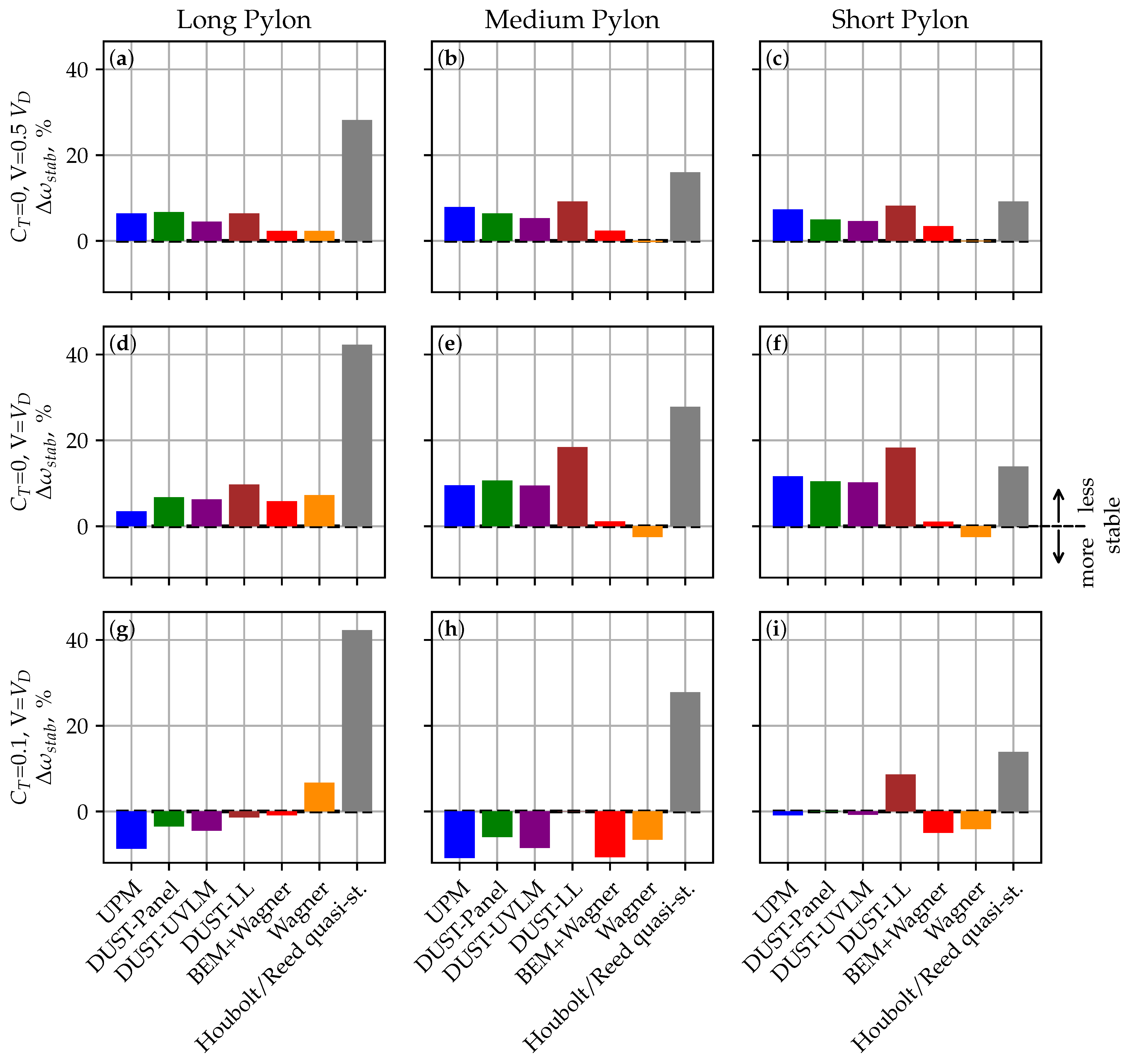
• For all configurations investigated, the Houbolt/Reed method yields the more stable (and thus less conservative) whirl flutter predictions for zero thrust than the mid-fidelity methods. If the Houbolt/Reed method is applied in its quasi-steady form (without Theodorsen correction), it results in the most unstable system, but unsteady aerodynamic predictions are far away from the other methods investigated in this comparison. Despite yielding the least conservative stability predictions, the Houbolt/Reed method was used successfully for the design and certification of several propeller aircraft in the past. This fact could be explained by conservatism in the designs or other stabilizing effects (such as blade elasticity) offsetting the destabilizing effect found. Further research is necessary to compare to experimental data or high-fidelity numerical test cases without the assumptions used in this study to identify the correct modeling approach.
• The stability predictions for systems with thrust are all more stable than the zero-thrust operating points, which confirms previous studies in the literature. The stabilizing effect can mainly be associated with the tilting torque vector. Although not checked in this study, this effect probably extends into the region of negative thrust/torque, which is believed to have a destabilizing effect and could thus be important for concepts that use propellers in conjunction with recuperation, as negative torque might destabilize the system.
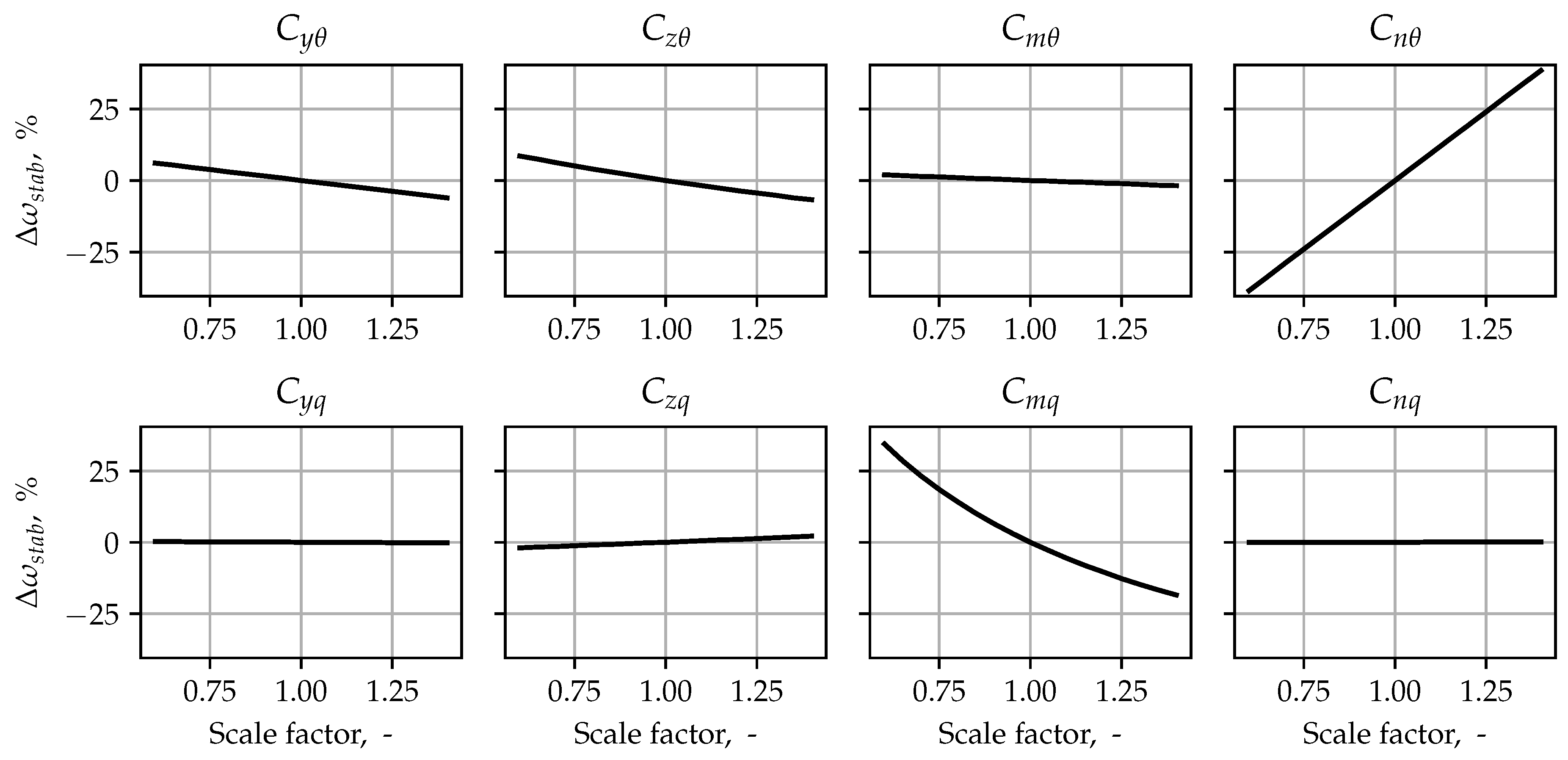
• To analyze the reasons for a variation in whirl flutter predictions when changing parameters, it is not sufficient to look at individual hub load components (e.g., only into the destabilizing term, $M_{z\theta }$). Changes in several components may cancel each other out, as some load components (or derivatives in the linearized approach) have a stabilizing and others a destabilizing effect. For the same reason, as results of the Wagner method demonstrated, general over- or under-prediction of unsteady aerodynamic loads does not necessarily result in large changes in whirl flutter stability.
• The transfer matrix method gives valuable insights into the unsteady aerodynamics of propellers, as it allows for an assessment of the change in individual hub load components with frequency and among different methods. This frequency dependency can then be transferred to frequency-domain flutter analysis, giving a proper unsteady representation of the propeller in the (whirl) flutter analysis process of, e.g., turboprop aircraft.
• Regarding the comparison of individual aerodynamic methods, the different mid-fidelity methods showed in general good agreement in unsteady aerodynamic and stability predictions. Among the low-fidelity methods, the BEM+Wagner method was, in most cases, the closest one to the mid-fidelity methods regarding unsteady aerodynamics. Regarding stability, it could give the same trends but had larger quantitative differences from the mid-fidelity methods.

Despite the comparison of different methods, operating points and structural configurations, some limitations apply to this work (see Section 2.2). Although delving into the detailed impact of the limitations on the outcomes is beyond the scope of this paper, recommendations for future research are provided to support additional investigations. The main limitation with respect to practical applications in whirl flutter analysis is the assumption of linear airfoil polars and incompressible flow in this work. Changes in the local airfoil polars (either due to steady angle of attack or compressibility) have already been shown to have a significant impact on whirl flutter predictions. The methods used in this paper allow one to account for this in different ways (nonlinear airfoil polars in the low-fidelity methods and lifting line, Prandtl–Glauert compressibility correction in the others). CFD simulations could give a good reference for compressible unsteady aerodynamic predictions. Future work could compare those to the different correction approaches to extend the findings of this work into the compressible regime. In general, even high-fidelity CFD predictions need to be validated with experimental data (either with forced-motion experiments or propeller whirl flutter tests on a reference configuration) to validate the findings. These studies (either high-fidelity numerical or experimental ones) could also lift the assumptions on aerodynamic interaction effects of the spinner, nacelle and wing.

To further shed a light on the sensitivity of whirl flutter prediction with regards to input parameters, a structured uncertainty quantification approach could be applied.

Regarding configurations, the main limitations are the geometry and operating points used. Although representative for a turboprop propeller, the advance ratios are still quite high; results might, therefore, not be applicable to new configurations, e.g., urban air mobility concepts. Propellers in this type of configuration operate under smaller advance ratios but at higher angles of attack and under higher loading, where different effects might play a role. The geometry of the propeller blades remained unchanged in this study. However, as mentioned in the literature, factors like blade aspect ratio and sweep are known to influence aerodynamic predictions, as well as whirl flutter stability. These parameters could be subjected to variations in future parameter studies to assess their impact and the prediction capabilities of the different methods. The results in this paper give valuable insights into the performance of different aerodynamic modeling techniques on whirl flutter stability predictions. They can be used by flutter engineers to choose a method based on requirements for conservatism and computational time. For final modeling guidelines, however, further validation studies are required.

References

1. Reed, W.H. Propeller-rotor whirl flutter: A state-of-the-art review. J. Sound Vib. 1966, 4, 526–544. [Google Scholar] [CrossRef]
2. Kunz, D.L. Analysis of Proprotor Whirl Flutter: Review and Update. J. Aircr. 2005, 42, 172–178. [Google Scholar] [CrossRef]
3. Hrycko, G. Design Of The Low Vibration Turboprop Powerplant Suspension System for The DASH 7 Aircraft. SAE Trans. 1983, 92, 133–145. [Google Scholar]
4. Cecrdle, J. Whirl flutter-related certification according to FAR/CS 23 and 25 regulation standards. In Proceedings of the International Forum on Aeroelasticity and Structural Dynamics (IFASD), Savannah, GA, USA, 10–13 June 2019. [Google Scholar]
5. Houbolt, J.C.; Reed, W.H., III. Propeller-nacelle whirl flutter. J. Aerosp. Sci. 1962, 29, 333–346. [Google Scholar] [CrossRef]
6. Donham, R.; Watts, G. Lessons learned from fixed and rotary wing dynamic and aeroelastic encounters. In Proceedings of the 41st Structures, Structural Dynamics, and Materials Conference and Exhibit, Atlanta, GA, USA, 3–6 April 2000. [Google Scholar] [CrossRef]
7. Ribner, H.S. Propellers in Yaw; NACA Wartime Report 3L09; NACA: Langley Field, VA, USA, 1943. [Google Scholar]
8. Bland, S.R.; Bennett, R.M. Wind-Tunnel Measurements of Propeller Whirl-Flutter Speeds and Static-Stability Derivatives and Comparison with Theory; NASA Technical Note NASA TN D-1807; NASA Langley Station: Hampton, VA, USA, 1963.
9. Rodden, W.; Rose, T. Propeller/nacelle whirl flutter addition to MSC/Nastran. In Proceedings of the 1989 MSC World User’s Conference, Anaheim, CA, USA, 26–27 January 1989. [Google Scholar]
10. Cecrdle, J. Analysis of Twin Turboprop Aircraft Whirl-Flutter Stability Boundaries. J. Aircr. 2012, 49, 1718–1725. [Google Scholar] [CrossRef]
11. Cecrdle, J. Whirl Flutter of Turboprop Aircraft Structures; Elsevier: Amsterdam, The Netherlands, 2015; ISBN 978-1-78242-185-6. [Google Scholar] [CrossRef]
12. Koch, C. Parametric whirl flutter study using different modelling approaches. CEAS Aeronaut. J. 2021, 13, 57–67. [Google Scholar] [CrossRef]
13. Böhnisch, N.; Braun, C.; Koschel, S.; Muscarello, V.; Marzocca, P. Dynamic aeroelasticitiy of wings with distributed propulsion systems featuring a large tip propeller. In Proceedings of the International Forum on Aeroelasticity and Structural Dynamics (IFASD), Madrid, Spain, 13–17 June 2022. [Google Scholar]
14. Böhnisch, N.; Braun, C.; Muscarello, V.; Marzocca, P. A Sensitivity Study on Aeroelastic Instabilities of Slender Wings with a Large Propeller. In Proceedings of the AIAA SCITECH 2023 Forum, National Harbor, MD, USA, 23–27 January 2023. [Google Scholar] [CrossRef]
15. Koch, C.; Koert, B. Including Blade Elasticity into Frequency-Domain Propeller Whirl Flutter Analysis. J. Aircr. 2023; in press. [Google Scholar] [CrossRef]
16. Smith, H.R. Engineering Models of Aircraft Propellers at Incidence. Ph.D. Thesis, University of Glasgow, Glasgow, UK, 2015. [Google Scholar]
17. Fei, X.; Litherland, B.L.; German, B.J. Development of an Unsteady Vortex Lattice Method to Model Propellers at Incidence. AIAA J. 2021, 60, 176–188. [Google Scholar] [CrossRef]
18. Ortun, B.; Boisard, R.; Martino, I.G. Assessment of propeller 1P loads predictions. Int. J. Eng. Syst. Model. Simul. 2012, 4, 36–46. [Google Scholar] [CrossRef]
19. Bousquet, J.M.; Gardarein, P. Improvements on computations of high speed propeller unsteady aerodynamics. Aerosp. Sci. Technol. 2003, 7, 465–472. [Google Scholar] [CrossRef]
20. Hoover, C.B.; Shen, J. Parametric Study of Propeller Whirl Flutter Stability with Full-Span Model of X-57 Maxwell Aircraft. J. Aircr. 2018, 55, 2530–2537. [Google Scholar] [CrossRef]
21. Hoover, C.B.; Shen, J. Fundamental understanding of propeller whirl flutter through multibody dynamics. In Proceedings of the AIAA Scitech 2019 Forum, San Diego, CA, USA, 7–11 January 2019. [Google Scholar] [CrossRef]
22. Cocco, A. Comprehensive Mid-Fidelity Simulation Environment for Aeroelastic Stability Analysis of Tiltrotors with Pilot-in-the-Loop. Ph.D. Thesis, Politecnio di Milano, Milan, Italy, 2022. [Google Scholar]
23. Corle, E.; Floros, M.; Schmitz, S. On the Influence of Inflow Model Selection for Time-Domain Tiltrotor Aeroelastic Analysis. J. Am. Helicopter Soc. 2021, 66, 1–12. [Google Scholar] [CrossRef]
24. Wang, Z.; Chen, P. Whirl flutter analysis with propeller aerodynamic derivatives computed by unsteady vortex lattice method. In Proceedings of the 56th AIAA/ASCE/AHS/ASC Structures, Structural Dynamics, and Materials Conference, Kissimmee, FL, USA, 5–9 January 2015. [Google Scholar] [CrossRef]
25. Gennaretti, M.; Greco, L. Whirl flutter analysis of prop-rotors using unsteady aerodynamics reduced-order models. Aeronaut. J. 2008, 112, 261–270. [Google Scholar] [CrossRef]
26. Koch, C. Whirl flutter stability assessment using rotor transfer matrices. In Proceedings of the International Forum on Aeroelasticity and Structural Dynamics (IFASD), Madrid, Spain, 13–17 June 2022. [Google Scholar]
27. Gori, R.; Serafini, J.; Molica Colella, M.; Gennaretti, M. Assessment of a state-space aeroelastic rotor model for rotorcraft flight dynamics. CEAS Aeronaut. J. 2016, 7, 405–418. [Google Scholar] [CrossRef]
28. Cecrdle, J. Influence of propeller blade lift distribution on whirl flutter stability characteristics. Int. J. Aerosp. Mech. Eng. 2014, 8, 727–733. [Google Scholar]
29. Kunze, P. Evaluation of an unsteady panel method for the prediction of rotor-rotor and rotor-bodyinteractions in preliminary design. In Proceedings of the 41st European Rotorcraft Forum 2015, (ER), Munich, Germany, 1–4 September 2015; Volume 1, pp. 473–485. [Google Scholar]
30. Yin, J.; Ahmed, S. Helicopter main-rotor/tail-rotor interaction. J. Am. Helicopter Soc. 2000, 45, 293–302. [Google Scholar] [CrossRef]
31. Yin, J.; Van Der Wall, B.; Wilke, G. Rotor aerodynamic and noise under influence of elastic blade motion and different fuselage modeling. In Proceedings of the 40th European Rotorcraft Forum 2014, Southampton, UK, 2–5 September 2014; Volume 1, pp. 475–495. [Google Scholar]
32. Tugnoli, M.; Montagnani, D.; Syal, M.; Droandi, G.; Zanotti, A. Mid-fidelity approach to aerodynamic simulations of unconventional VTOL aircraft configurations. Aerosp. Sci. Technol. 2021, 115, 106804. [Google Scholar] [CrossRef]
33. Zanotti, A.; Savino, A.; Palazzi, M.; Tugnoli, M.; Muscarello, V. Assessment of a Mid-Fidelity Numerical Approach for the Investigation of Tiltrotor Aerodynamics. Appl. Sci. 2021, 11, 3385. [Google Scholar] [CrossRef]
34. Arnold, J.; Waitz, S. Using Multibody Dynamics for the Stability Assessment of a New Double-Swept Rotor Blade Setup. In Proceedings of the ERF 2018—44th European Rotorcraft Forum, Delft, The Netherlands, 18–21 September 2018. [Google Scholar]
35. Burton, T.; Jenkins, N.; Sharpe, D.; Bossanyi, E. Wind Energy Handbook, 2nd ed.; Wiley: Chichester, UK, 2011. [Google Scholar]
36. Verdonck, H.; Hach, O.; Polman, J.D.; Braun, O.; Balzani, C.; Müller, S.; Rieke, J. An open-source framework for the uncertainty quantification of aeroelastic wind turbine simulation tools. J. Phys. Conf. Ser. 2022, 2265, 042039. [Google Scholar] [CrossRef]
Figure 1. Simplified pylon model used in this work (a) together with a basic stability map (b) showing parameter ranges for whirl flutter, static divergence and stable areas, obtained by varying K θ and K ψ .
Applsci 14 00850 g001
Figure 2. Sensitivity of whirl flutter with respect to the individual propeller derivatives for varying scale factors.
Applsci 14 00850 g002
Figure 3. Flow chart for the blade lift and wake equilibrium.
Applsci 14 00850 g003
Figure 4. Chord and twist distributions of the blade (R = 1.25 m ).
Applsci 14 00850 g004
Figure 5. Propeller model and coordinate system used in this study.
Applsci 14 00850 g005
Figure 6. Comparison of steady blade loading for operating point C T = 0.1 , V = V D . The top plot shows the out-of-plane force distribution ( F x , in N/m) along the blade span. The bottom plot shows the corresponding tangential or in-plane blade loading ( F t a n ).
Applsci 14 00850 g006
Figure 7. Distribution of variation in out-of-plane blade forces and angle of attack during one revolution with steady disc pitch angle. (a) Local blade angle of attack perturbation due to disc pitch θ ; (b) Variation in out-of-plane force in UPM simulation.
Applsci 14 00850 g007
Figure 8. Comparison of the four in-plane hub load derivatives under steady disc pitch angle. The top row shows the y- and z-forces, and the second row, the y- and z-moments.
Applsci 14 00850 g008
Figure 9. Frequency-dependent transfer function from disc pitch to in-plane hub loads. The first row shows the real (solid lines) and imaginary (dashed lines) part of the force components, while the second row shows the moments. For better visibility, only UPM results are shown, representative of mid-fidelity codes.
Applsci 14 00850 g009
Figure 10. Comparison of the linearized derivatives. The dashed horizontal line marks the reference derivatives from the Houbolt/Reed method.
Applsci 14 00850 g010
Figure 11. Comparison of whirl flutter stability map predictions with different aerodynamic methods and for different pylon lengths. For the long pylon, the quasi-steady Houbolt/Reed results are outside the range at higher frequencies (5.5 Hz for equal stiffness).
Applsci 14 00850 g011
Figure 12. Comparison of stability measure relative to Houbolt/Reed among different methods at three operating points (rows) and for three pylon lengths (columns).
Applsci 14 00850 g012