Unraveling Convolution Neural Networks: A Topological Exploration of Kernel Evolution

Abstract

Convolutional Neural Networks (CNNs) have become essential in deep learning applications, especially in computer vision, yet their complex internal mechanisms pose significant challenges to interpretability, crucial for ethical applications. Addressing this, our paper explores CNNs by examining their topological changes throughout the learning process, specifically employing persistent homology, a core method within Topological Data Analysis (TDA), to observe the dynamic evolution of their structure. This approach allows us to identify consistent patterns in the topological features of CNN kernels, particularly through shifts in Betti curves, which is a key concept in TDA. Our analysis of these Betti curves, initially focusing on the zeroth and first Betti numbers (respectively referred to as Betti-0 and Betti-1, which denote the number of connected components and loops), reveals insights into the learning dynamics of CNNs and potentially indicates the effectiveness of the learning process. We also discover notable differences in topological structures when CNNs are trained on grayscale versus color datasets, indicating the need for more extensive parameter space adjustments in color image processing. This study not only enhances the understanding of the intricate workings of CNNs but also contributes to bridging the gap between their complex operations and practical, interpretable applications.

1. Introduction

Convolutional Neural Networks (CNNs), a key part of deep learning methodologies, have become a part of many areas of daily life because of their significant advancements in computer vision. Introduced as early as the 1980s [1], the concept of CNNs gained significant attention following the ImageNet Large Scale Visual Recognition Challenge (ILSVRC) in 2012 [2,3], becoming a leading tool in computer vision tasks. CNNs employ weight sharing and pooling layers, techniques that preserve data features while simultaneously reducing computational complexity, thereby significantly reducing the need for computational power and enhancing the efficiency of the network structure. However, the lack of transparency and interpretability inherent in neural networks has slowed down the widespread acceptance and approval of CNNs by relevant institutions, despite their significant advancements and community applications. This lack of interpretability can pose significant ethical problems in the application of CNNs [4,5,6,7].

Aiming to enhance the interpretability of neural networks, researchers have proposed a series of methods. These methods are broadly classified into local explanations and global explanations. Local explanations focus on the behavior of models on specific inputs or neurons, aiming to uncover the mechanisms through which models make predictions on specific samples. For instance, generalizable complex model interpretability methods, such as LIME [8] and SHAP [9], are quite popular. LIME creates an interpretable local linear model around input data to approximate the behavior of complex models in that locality, while SHAP assigns importance values to each sample feature based on game theory, thus explaining individual predictions. Additionally, visualizing the features and behaviors of neural network models also falls under local explanations. For example, in the literature, the authors of [10] visualize the outputs of hidden layer activation functions to observe the learned features, aiding in understanding how models recognize different types of input data. Local explanation methods focus on how specific samples or neurons operate in neural networks, not revealing more generalized patterns of neural networks. In contrast, global explanations aim to study the overall behavior and characteristics of models, uncovering the general working principles of the models. For example, through theoretical analysis, some studies have aimed to understand the capacity, stability, and generalization abilities of models [4,11,12]. Other works test the performance and robustness of models by constructing adversarial examples [13].

In recent years, there has been growing interest in utilizing topological tools, such as persistent homology, to interpret the behavior of neural networks [14,15,16,17,18,19], which fits within the field of Topological Data Analysis (TDA). These methods offer valuable insights into the internal representations and dynamics of neural networks by analyzing their topological properties. Typically, this analysis involves extracting features from neural networks, such as neuron activations, weights, or other network attributes, which can be represented as high-dimensional point clouds or graphs. Topological techniques, including persistent homology and simplicial complexes, are then applied to extract and analyze the topological information encoded within these high-dimensional structures [20,21]. Through this process, researchers gain a deeper understanding of the network’s behavior and can leverage the obtained insights to improve network architecture, optimize hyper-parameters, enhance performance, reduce overfitting, or increase interpretability.

One aspect of the work focuses on analyzing the feature space of neural networks. Bianchini and Franco Scarselli [22] utilize topological concepts to measure the complexity of neural networks. They calculate the Betti numbers of decision boundaries in the data space to evaluate the complexity of neural networks. Their research provides upper and lower bounds for the complexity of shallow and deep networks with the same number of hidden units, highlighting the higher complexity of deep structures. Guss and Salakhutdinov [23] investigate the relationship between the topological complexity of datasets and the capacity of neural networks. By understanding the topological features of datasets, more efficient and smaller-scale network architectures can be designed, reducing computational resources and training time. Another line of research involves the visualization of neural networks using the Mapper algorithm. Goldfarb [24] applies the Mapper algorithm to visualize test datasets in deep neural network models. By clustering the activations of the test set on the neural network, they identify clusters representing misclassified samples, which provide insights into areas where the network’s performance can be improved. Gabrielsson and Carlsson [25,26] visualize the convolutional kernels of well-trained CNNs using the Mapper algorithm. They observe that the point cloud formed by the kernels exhibits a “ring” structure in the parameter space. This finding suggests that convolutional kernels tend to form a simple topological structure during the network learning process. Furthermore, they propose the notion of “topological simplicity” as a measure of network generalization performance, comparing the persistence lengths of one-dimensional homology classes.

Other works also explore the parameter space analysis of neural networks. Rieck et al. [15] introduce a method to measure the complexity of neural network structures. By constructing a weighted graph, where neurons are considered vertices and connections are considered edges, they use persistent homology to quantify the 0-dimensional topological information of the graph. This complexity measure can monitor the impact of regularization techniques, such as dropout and batch normalization, during the network training process and serve as an indicator of overfitting. Watanabe and Yamana [16] view the entire neural network as a directed weighted graph and apply the construction of Clique complexes to capture the topological features of the parameter space. This approach allows the introduction of higher-dimensional topology and provides insights into the neural network’s structural organization and hierarchy. These studies demonstrate the diverse applications of topological analysis in interpreting neural networks, assessing their complexity, and guiding network design, optimization, and generalization.

Our research specifically investigates the dynamic topological evolution of CNN kernels throughout the learning process. We analyze the shifts in the Betti-0 and Betti-1 curves of convolutional kernels, revealing patterns that highlight the network’s learning dynamics and decision-making process. A key focus is the distinct topological adjustments observed when CNNs are trained on grayscale versus color datasets, emphasizing the need for significant parameter space modifications for color image learning. Our contributions are significant in two ways: (i) unveiling the dynamic topological patterns in CNN kernels during the iterative learning process and (ii) demonstrating how these topological changes can serve as indicators of effective learning within the network and influence the overall performance. This insight not only deepens our understanding of CNN internals but also opens new pathways for optimizing their design and application in complex scenarios.

2. Theoretical Background

This section establishes the theoretical framework crucial to our exploration of CNN kernels through the lens of TDA. We begin by introducing the concept of a simplicial complex, a foundational structure in algebraic topology, which plays an important role in analyzing and understanding the connectivity patterns within topological spaces. Building on this, we explore the concepts of homology and persistent homology, highlighting their roles in quantifying and tracking the evolution of topological features over different scales. We then explore various representation methods for persistent homology—such as persistence diagrams, barcode plots, and Betti curves—that enable us to effectively visualize and interpret these complex topological characteristics. This theoretical overview will provide the necessary tools and perspectives to decode the complex behaviors of CNNs in our research.

2.1. Simplicial Complex

A simplicial complex, a key construct in algebraic topology, facilitates the study of the connectivity and shape of topological spaces. It is built from simpler geometric objects known as simplices. A simplex, the most elementary form in a simplicial complex, in an n-dimensional Euclidean space, is the convex hull formed by $(n+1)$ points that do not all lie in the same $(n-1)$-dimensional space. For instance, a 0-simplex is a point, a 1-simplex is a line segment connecting two points, and a 2-simplex is a triangle formed by three non-collinear points. By combining these simplices following specific rules, simplicial complexes of various dimensions and shapes can be created. These complexes offer a combinatorial approach to represent and study the properties of topological spaces using algebraic and combinatorial techniques.

In TDA, simplicial complexes are essential for analyzing and understanding the topological features of datasets. They provide a combinatorial representation of the data space, constructed based on the pairwise distances or similarities among data points. In these complexes, a k-dimensional simplex corresponds to a subset of $(k+1)$ mutually close or similar data points, representing different levels of connectivity or interactions among them. Upon constructing a simplicial complex, various topological features can be identified and analyzed. This includes computing Betti numbers, indicative of the number of topological features of different dimensions such as connected components, holes, or voids. Additionally, other topological invariants such as persistent homology are computed to determine and quantify the persistence of these features across various scales.

2.2. Homology and Persistent Homology

Homology, another fundamental concept in algebraic topology, provides a means by which to count the number of holes in each dimension in a space. More precisely, it associates a sequence of abelian groups, known as homology groups, with each topological space. These groups offer an intuitive count of n-dimensional holes; for instance, the 0th homology group counts connected components, the 1st counts “loops”, and the 2nd counts voids.

Persistent homology, a specialized form of homology used in TDA, introduces an additional dimension: scale, or persistence. Its main objective is to measure the persistence of topological features, such as connected components (0-dimensional holes), loops (1-dimensional holes), and voids (2-dimensional holes), across various scales [27]. This method helps in distinguishing significant features from noise by quantifying how long each topological feature persists as the scale changes.

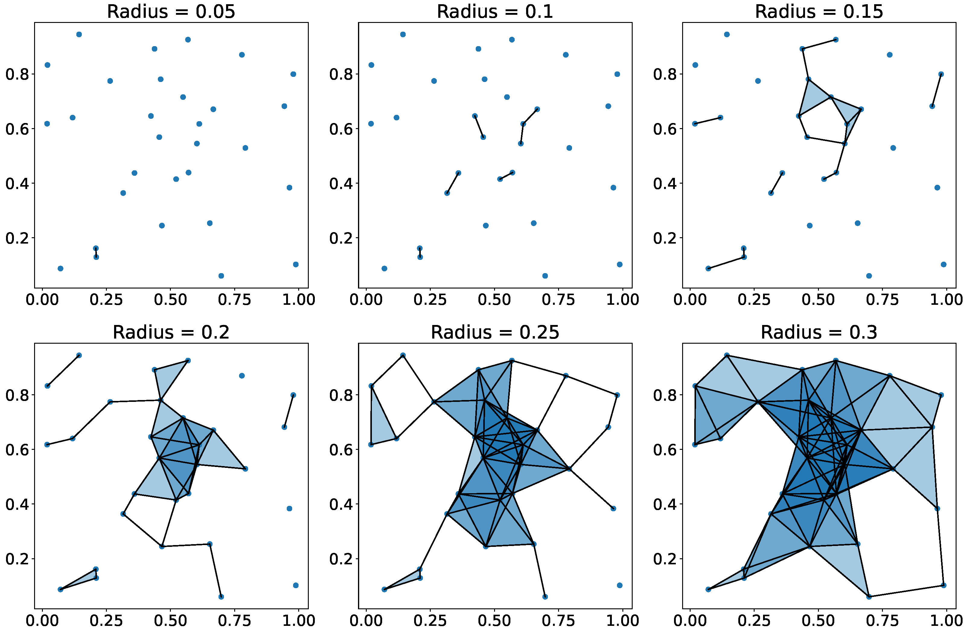
The process begins with a point cloud dataset, around each point of which balls of a certain radius are grown (as illustrated in Figure 1). As the radius increases, these balls intersect, forming shapes and allowing the tracking of the emergence and disappearance of homological features such as connected components or holes. These intersections form simplices: a 1-simplex (edge) is formed when the balls of two points overlap, a 2-simplex (triangle) forms from three overlapping points, and so forth. With the continued increase in radius, more simplices are added, creating a sequence of spaces known as a filtration. This filtration, alongside the corresponding homology groups, captures the evolving topological features of the data as the scale parameter (radius) changes.

2.3. Representations of Persistent Homology

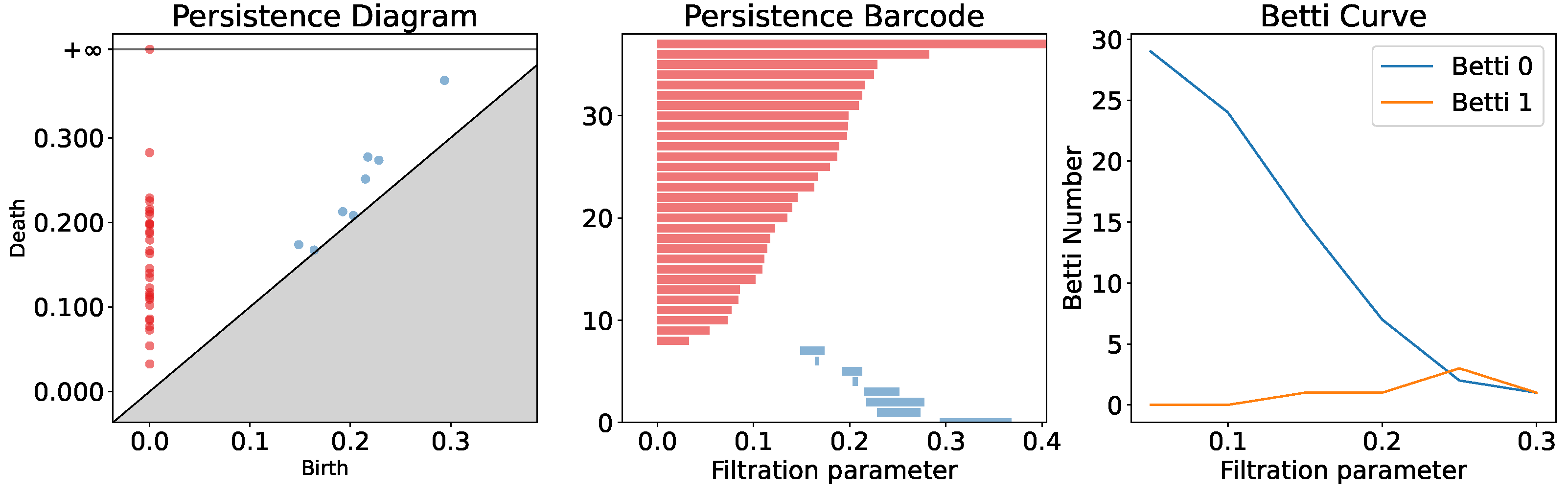
Persistent homology results, illustrated through the evolution of a simplicial complex with an increasing radius in Figure 1, can be visually represented through persistence diagrams, barcode plots, or Betti curves [28], as shown in Figure 2. In the persistence diagram (left panel of Figure 2), each point represents a topological feature, with the vertical position indicating when the feature appears and the horizontal position indicating when it becomes insignificant. Red points in this diagram correspond to the most basic connectivity structures, while blue points represent primary cycles or loops within the space. Similarly, the barcode plot (middle panel of Figure 2) uses red bars to denote the persistence of the basic connectivity structures and blue bars for the primary cycles, with the length of each bar representing the lifespan of the corresponding feature within a specific filtration range.

The Betti curve (right panel of Figure 2) is another visualization tool in persistent homology. Unlike persistence diagrams or barcodes that summarize feature persistence across filtration levels, Betti curves provide a detailed view of the evolution of individual Betti numbers. Betti numbers denote the count of k-dimension holes in a topological space, such as the number of connected components (0th Betti number), 1-dimensional loops (1st Betti number), and so on.

A Betti curve plots Betti numbers against the filtration level, illustrating how the count of topological features changes with the filtration. This curve offers insights into the development and disappearance of topological features at varying scales. The Betti curve provides a more granular analysis of individual Betti numbers, complementing the overall view provided by persistence diagrams or barcodes. It enables a deeper understanding of the topological structure of the data, revealing intricate patterns and transitions in the formation of holes across different dimensions.

While persistent homology provides a robust framework for analyzing topological structures, the exploration of CNNs’ topological complexity is not limited to this method alone. Specifically, multidimensional persistent homology broadens the scope of traditional persistent homology, enabling the examination of data’s topological features through a multi-faceted lens [29]. Furthermore, the Mapper algorithm reveals the shape structure of data by creating a simplified representation. It is particularly suited for exploring the geometric and topological properties of high-dimensional data [30]. The application of the Mapper algorithm in the context of CNN kernels may uncover new insights into their high-dimensional learning processes, highlighting geometric and topological features that influence learning effectiveness and efficiency. In pursuit of clarity and to lay the groundwork for our analysis, we initially embrace Betti curves derived from persistent homology to map out and scrutinize the topological features of CNN kernel spaces. This approach simplifies our initial investigations and provides a comprehensive platform for delving into the evolutionary patterns of these features throughout the training process.

2.4. Betti Curves of Convolutional Kernels

Here, we outline the main idea underlying our research. We analyze the evolution of convolutional kernels in CNNs through a topological approach. Initially, we reshape each 3 × 3 convolutional kernel into a nine-dimensional vector, effectively representing each kernel as a point within a nine-dimensional Euclidean space. This transformation allows us to create a point cloud representation of the convolutional kernels. Utilizing the concept of persistent homology, we then quantify the topological “shape” of these kernels, identifying consistent features and patterns that prevail across different scales. This is achieved by calculating the persistent homology of the point cloud, which elucidates the number and nature of “holes” or voids within the topological structure of CNN kernels.

Key to our analysis is the use of Betti curves, which provide a graphical representation of these topological features. These curves enable us to track and visualize the changes in the convolutional kernels’ topology as the training of the CNN progresses. The dynamic alterations in the weights of the kernels during training lead to changes in their topological structure. By generating and examining Betti curves at each iteration of the training process, we gain deep insights into the evolving patterns and complexities of the kernels’ topological landscape. It offers a unique perspective on how convolutional kernels adapt and modify their structures in response to the learning process.

3. Experiments

In this section, we detail our experimental approach, designed to explore the dynamic topological evolution of convolutional kernels in neural networks. Our methodology involves training two distinct neural network architectures on a carefully curated selection of datasets. These datasets range from grayscale to color images, including a variety of content types to thoroughly evaluate the universal patterns of topological changes in the convolutional kernel space. In this series of experiments, we aim to investigate the topological changes in convolutional kernels and the relationship between the topological evolution of convolutional kernels and neural network performance, as measured by traditional performance metrics such as accuracy, loss, and the area under the receiver operating characteristic (ROC) curve.

3.1. Experiment Setup

The experimental setup is designed to examine the topological changes in convolutional kernels under different learning scenarios. We selected three distinct categories of datasets: grayscale images, color images, and synthetic images, each representing unique challenges in color channels, classification complexity, and specific use cases. The details of these datasets are summarized in

Table 1. The detailed descriptions of three categories of datasets.

Image	Dataset Name	Image Size	Categories	Dataset Content	Rename
Grayscale Image (A)	MNIST a	28 × 28	10	Handwritten digits (0–9)	A1
	Kuzushiji-MNIST b	28 × 28	10	Kuzushiji characters	A2
	Fashion-MNIST c	28 × 28	10	Various clothing items	A3
Color Image (B)	CIFAR-10 d	32 × 32	10	Various objects and animals	B1
	BALL-10 e	128 × 128	10	Different sports balls	B2
	CIFAR-100 f	32 × 32	100	Various objects and animals	B3
	BUTTERFLY-100 g	128 × 128	100	Different butterfly species	B4
Synthetic Image (C)	NOISE-2 h	64 × 64	2	Synthesized colored noise	C1
	PURE-2 i	64 × 64	2	Uniform black and white images	C2

^a MNIST [31], ^b Kuzushiji-MNIST [32], ^c Fashion-MNIST [33], ^d CIFAR-10 [34], ^e BALL-10 https://www.kaggle.com/datasets/samuelcortinhas/sports-balls-multiclass-image-classification (accessed on 4 October 2023), ^f CIFAR-100 [34], ^g BUTTERFLY-100 https://www.kaggle.com/datasets/gpiosenka/butterfly-images40-species?select=test (accessed on 4 October 2023), ^h NOISE-2: Synthesized colored noise dataset, generated by the authors, ⁱ PURE-2: Dataset of uniform black and white images for testing, generated by the authors.

.

For this study, we employed two neural network architectures, Network I and Network II, to evaluate the consistency of our findings across different structural designs. While both networks share the same fully connected layers, they differ in their convolutional layers: Network I has three, and Network II includes an additional fourth layer. This differentiation allows us to assess the impact of convolutional layer complexity on learning outcomes. The architectural specifics and hyper-parameters for these networks are detailed in

Table 2. The detailed architecture and hyper-parameter selection of the neural networks. Here, H and W represent the height and width of the image after passing through the convolutional layer and Maxpooling.

Network	Hyper-Parameters	Layer 1	Layer 2	Layer 3	Layer 4	Fully Connected Layer 1	Fully Connected Layer 2
Network I	Convolution Kernel Size	3 × 3	3 × 3	3 × 3	N/A	N/A	N/A
	Dropout (p)	N/A	N/A	N/A	N/A	0.2	0.2
	Quantity	16	32	64	N/A	$64\times H\times W$	500
	Maxpooling	(2, 2)	(2, 2)	(2, 2)	N/A	N/A	N/A
	Layer Identifier	I1	I2	I3	N/A	FC1	FC2
Network II	Convolution Kernel Size	3 × 3	3 × 3	3 × 3	3 × 3	N/A	N/A
	Dropout (p)	N/A	N/A	N/A	N/A	0.2	0.2
	Quantity	16	32	64	32	$32\times H\times W$	500
	Maxpooling	(2, 2)	(2, 2)	(2, 2)	N/A	N/A	N/A
	Layer Identifier	II1	II2	II3	II4	FC1	FC2

.

The experimental procedure involved careful hyper-parameter selection based on insights from preliminary trials and dataset analyses. Key parameters included a batch size of 64 and a learning rate of 0.01, using the momentum optimization method for training. The networks were trained using PyTorch (version 2.0.1, developed by the PyTorch team) [35], and the Ripser tool (version 0.6.8, created by Christopher Tralie and Nathaniel Saul, sourced from the Scikit-TDA project) [36] was used for computations related to persistent homology and topological invariants.

3.2. Betti Curves on Diverse Datasets

The experiments, detailed in Table 1 and Table 2, involved training on diverse datasets (A, B, and C) using two distinct neural network architectures (I and II). The primary focus was analyzing how convolutional kernels evolve across these different learning scenarios.

3.2.1. Study on Grayscale Images (Category A)

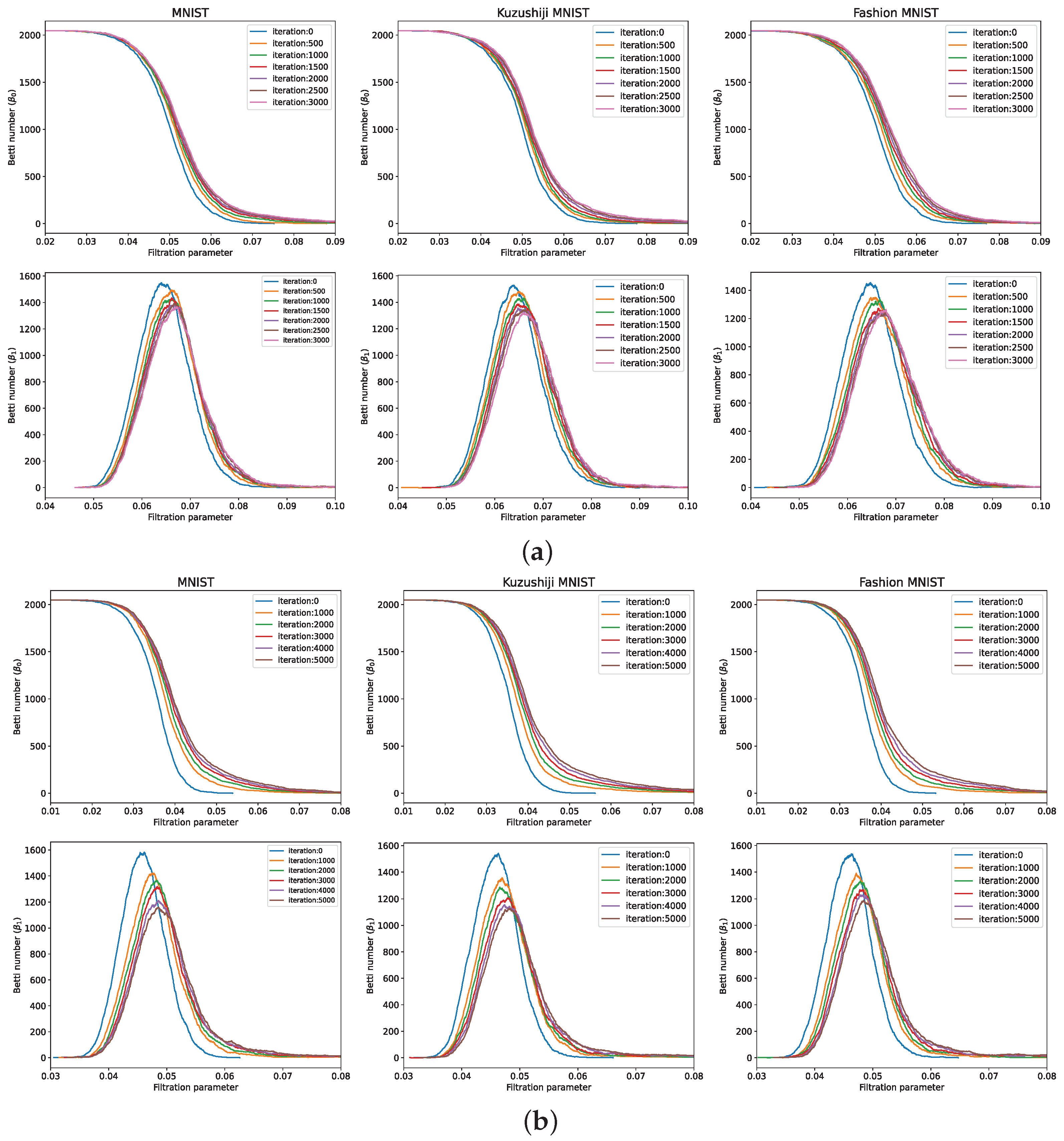
In the grayscale image category (A), we trained the networks on datasets such as MNIST, Kuzushiji-MNIST, and Fashion-MNIST. The analysis primarily targeted the second and third convolutional layers over 15,000 training iterations. Betti curves, representing the topological structure of 3 × 3 convolutional kernels, were computed at regular intervals to observe the evolution patterns. For networks with an additional fourth layer (A-II), the analysis was extended to cover this layer as well.

Figure 3 illustrates the Betti curve results for experiments A-I and A-II, conducted on grayscale image datasets. Each panel, corresponding to the MNIST, Kuzushiji-MNIST, and Fashion-MNIST datasets, shows the behavior of Betti curves over successive training iterations. A consistent trend is observed across both experimental conditions: the Betti-0 curve shifts rightward as the number of iterations increases, a pattern that becomes more apparent when early iterations are compared to later ones, indicating rapid initial changes in the topological structure that stabilize as training progresses. For the Betti-1 curve, as the number of iterations increases, the peak decreases, and the curve as a whole shifts rightward as well, indicating a reduction in the number of 1-dimensional loops within the kernel space as training progresses.

3.2.2. Study on Color Images (Category B)

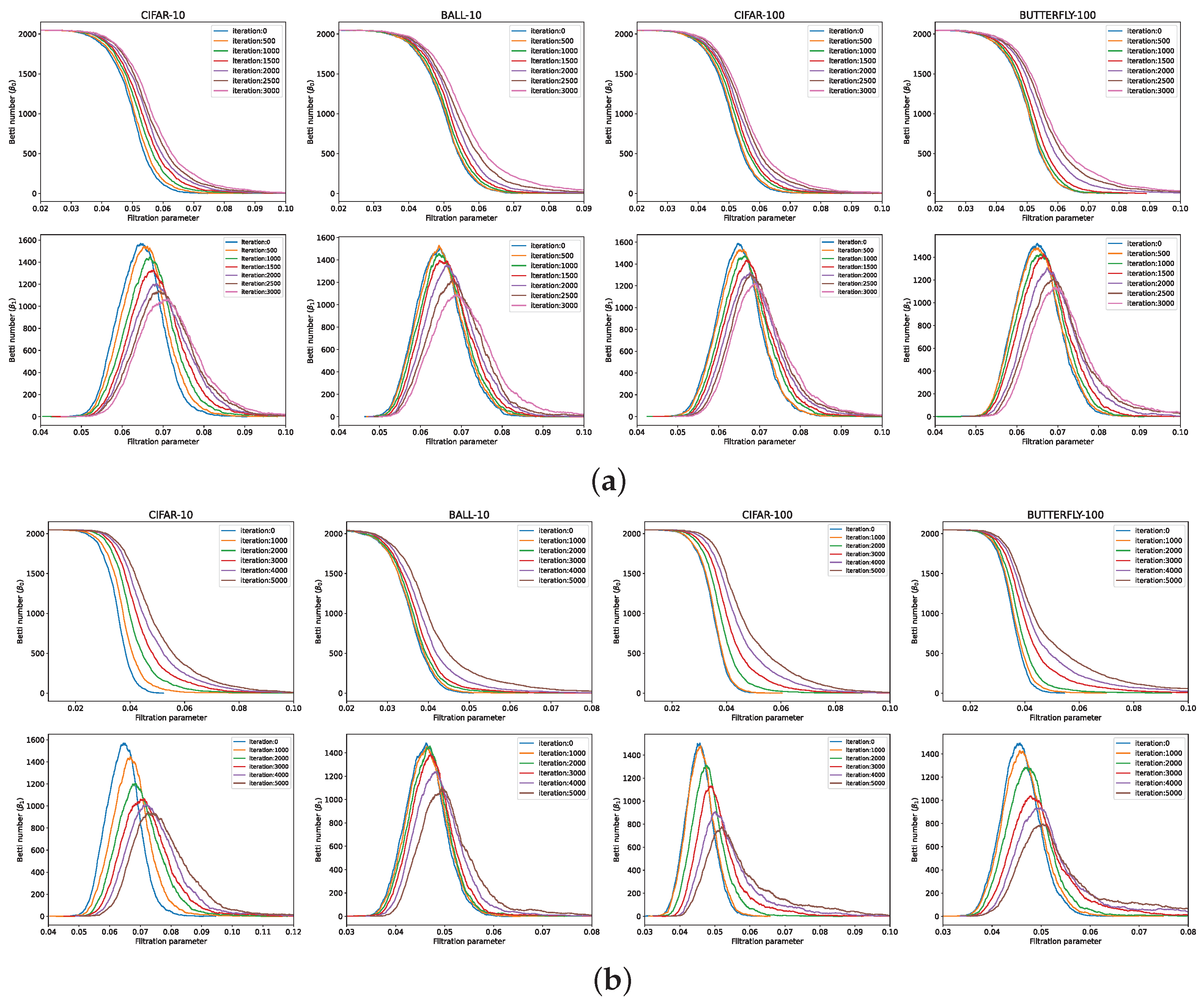
In the color image category (B), experiments were conducted on datasets such as CIFAR-10, BALL-10, and BUTTERFLY-100. Similar to the grayscale studies, the focus was on the evolution of convolutional kernels in the later layers of the networks. The analysis involved tracking the Betti curves throughout the course of the training to understand the topological changes.

Figure 4 showcases the Betti curves for Experiments B-I and B-II. These curves represent two distinct sets for each experiment, covering the CIFAR-10, BALL-10, and BUTTERFLY-100 datasets. Across both B-series experiments, the Betti curves exhibited consistent behaviors. The Betti-0 curve displayed a rightward shift with advancing iterations, while the Betti-1 curve exhibited an initial increase, subsequently followed by a decrease. There was a reduction in the peak values and a shift of the curve toward the right.

From the results of both experiments, a shared pattern emerges in the Betti curves, consistently observed across different network architectures, classification targets, and the convolutional layers in focus. This pattern is clear in the analysis of Betti curves from both grayscale (Figure 3) and color (Figure 4) image datasets. Specifically, in both sets of experiments, the Betti-0 curve consistently shifts rightward as training iterations increase. Concurrently, the Betti-1 curve demonstrates an initial rise followed by a decline, accompanied by a reduction in peak values and a corresponding rightward shift. This trend becomes more pronounced when early iterations are compared to later ones, indicating an initial rapid evolution in the topological structure that stabilizes over time.

3.2.3. Evaluation Using Synthetic Images (Category C)

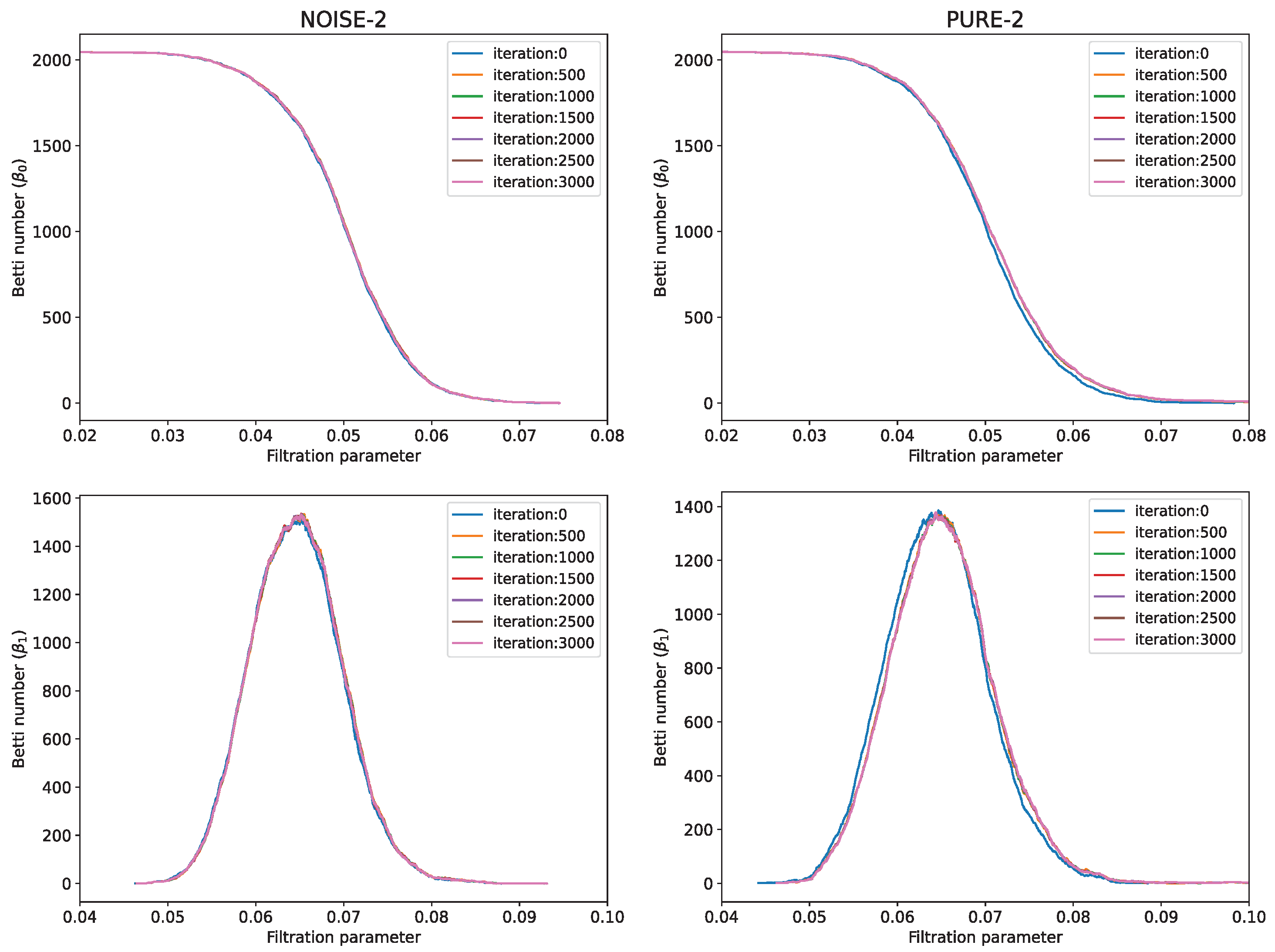
To assess whether the observed patterns were specific to certain dataset characteristics, we conducted experiments with synthetic images, including datasets with randomly generated noisy images and images with uniform color. This approach allowed us to compare the Betti curves and identify any special or unusual patterns, revealing insights into how the networks learn.

The results, as shown in Figure 5, provide clear contrasts. In the case of the NOISE-2 dataset, the Betti-0 and Betti-1 curves are fairly consistent across iterations, hinting at a stable topological structure. However, this consistency might suggest that the network’s learning from these datasets is not very efficient, as seen by the absence of significant, regular patterns mentioned before in the Betti curves. The natural randomness in the noisy dataset likely makes it difficult for the network to process and adapt. On the other hand, the PURE-2 dataset shows small but noticeable changes in the Betti-0 and Betti-1 curves compared to NOISE-2. Even with these changes, a level of steadiness is kept throughout the iterations. This indicates that minor modifications in the convolutional kernels were sufficient for achieving the desired outcomes, leading to minimal alterations in the Betti curves. Compared to the noisy dataset, this dataset exhibits a certain level of pattern and regularity, hinting at a more effective network training process.

Our findings show that clear, regular patterns in the Betti curves suggest the network is training well. If we see these regular patterns, it means that the network is learning and adjusting as expected. However, if the curve stays pretty much the same and does not have clear patterns, it could mean the network is having trouble learning from and adjusting to the data.

3.3. Comparative Analysis of Betti and ROC Curves across Iterations

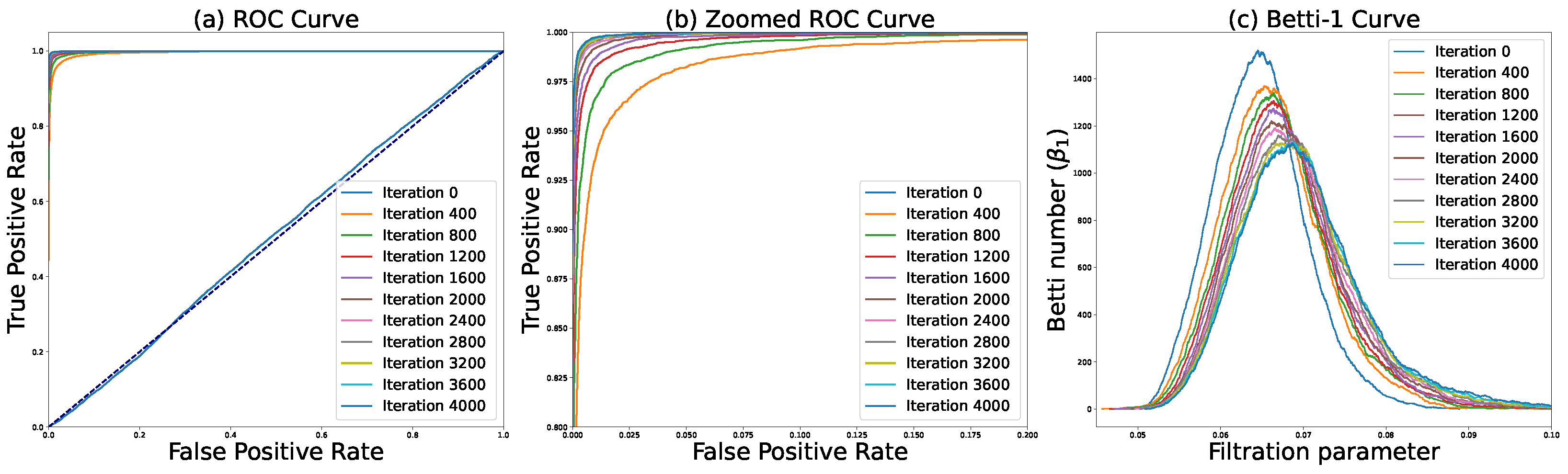
To provide deeper insight into the relationship between the topological changes in the convolutional kernels and the performance of the CNN models, we conducted an experiment to track the development of the ROC curve—a reliable performance metric for classification models—over the duration of network training. The ROC curve serves as a graphical representation of a model’s diagnostic ability, plotting the true positive rate against the false positive rate at various threshold settings. By examining the trajectory of the ROC curve along with the concurrent topological shifts in the convolutional kernels, encapsulated by the Betti-1 curves, our goal was to discern the interplay between a CNN’s learning process and the evolution of its internal structural complexity.

The experimental results are presented in Figure 6, which includes a comparative analysis of Betti and ROC curves across different training iterations. The ROC curve (Figure 6a) shows the trade-off between the true positive rate and the false positive rate. To enhance the clarity of our ROC analysis, we have included a zoomed-in view of the ROC curve (Figure 6b), which allows for a detailed examination of the model’s performance in the critical threshold range. The progression toward the upper left corner with increasing iterations indicates an improvement in model accuracy.

The Betti-1 curve (Figure 6c) illustrates the evolution of the topological features within the convolutional layers of the CNN. Throughout the course of training iterations, the Betti-1 curve undergoes significant changes, suggesting a refinement in the topological complexity of the kernel space. Notably, the peak of the Betti-1 curve becomes less pronounced with more iterations, implying that the network is optimizing its internal representations. A correlation analysis between the shifts in the Betti-1 curve and the ROC curve demonstrates that as the Betti-1 curve stabilizes (indicating a mature kernel topology), the area under the ROC curve (AUC) increases. This suggests that the topological changes in the convolutional kernels are reflective of the CNN’s learning progress.

3.4. Quantitative Analysis of Betti Curves

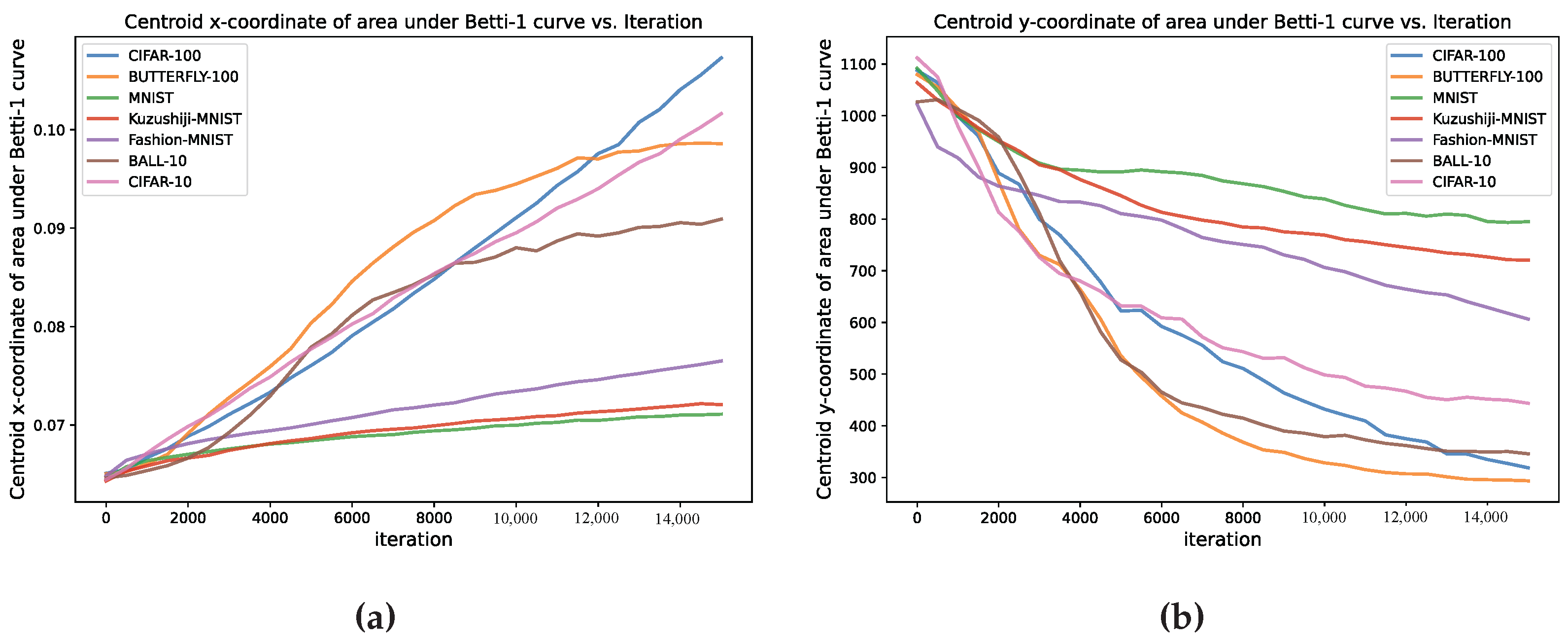
Building upon the insights gathered from the studies on grayscale, color, and synthetic images, we conducted another experiment that aimed to quantitatively analyze the evolving topological features of the convolutional kernels through a new lens—the centroids of Betti curves. This phase focused on the datasets from Categories A and B. The objective was to calculate the centroids of the Betti-1 curves, which had been tracked throughout the training process for each dataset. To achieve this, we employed Simpson’s Rule—a well-known method for its accuracy in numerical integration. This method helped us accurately determine the coordinates of the Betti curve centroids. The process included collecting the Betti curves at various stages of the training iterations. For each of these curves, we calculated the centroid coordinates, which provided us with a two-dimensional representation (x and y coordinates) of the curve’s central point. These coordinates were then plotted against the number of training iterations, creating a dynamic trajectory that illustrated the evolving topological structure in the kernel space as the network progressed.

The experimental results, as shown in Figure 7a,b, illustrate the changes in the centroid coordinates of the Betti-1 curves across iterations for various datasets. Figure 7a displays the trajectory of the x-coordinate of centroids under the Betti-1 curve throughout the course of the training iterations. It can be observed that the x-coordinates for color image datasets, such as CIFAR-10, CIFAR-100, and BUTTERFLY-100, show a more pronounced increase compared to those of grayscale image datasets, such as MNIST, Kuzushiji-MNIST, and Fashion-MNIST. Similarly, in Figure 7b presents the trajectory of the y-coordinate of centroids under the Betti-1 curve versus iterations. Here, too, the color image datasets demonstrate a more substantial decrease in the y-coordinates over iterations than the grayscale datasets.

The results indicate that the topological changes in convolutional kernels, represented by centroid shifts for color images, are more significant in both the x and y directions compared to those for grayscale images. This could imply that the convolutional networks are learning more complex features or adapting more extensively when trained on color images as opposed to grayscale images.

4. Conclusions

In this study, we observed a consistent pattern in the topological evolution of convolutional kernels throughout the iteration process of neural networks. Specifically, the Betti-0 curve persistently shifted rightward, indicating a steady progression. The Betti-1 curve is characterized by initially rising and then declining, marked by a diminishing peak and a gradual shift toward the right. Observing this pattern during training suggests that the neural network is learning effectively. Conversely, if this pattern is not evident, it may indicate obstacles in the learning process. Therefore, this pattern may serve as a potential indicator of effective learning within the network. Moreover, a notable difference was observed in the topological changes of convolutional kernels when trained on grayscale datasets, such as MNIST, Kuzushiji-MNIST, and Fashion-MNIST, compared to those trained on color datasets. The latter showed more significant topological adjustments, suggesting a need for more substantial modifications in the neural network’s parameter space to learn from color images.

Future research will involve the development of new methods to more effectively harness the observed topological changes for improving neural network performance and interpretability. This might include techniques for optimizing network structures or parameter-tuning strategies based on topological indicators. Additionally, our investigations will broaden beyond the scope of persistent homology, incorporating a wider array of analytical methods and tools. We are set to explore further methodologies, such as multi-dimensional persistence, and to employ specialized visualization tools, including the Mapper algorithm. These efforts are intended to facilitate a deeper analysis of the topological complexity inherent in CNN kernels, viewed from a multitude of angles.