
Spatial and Momentum Mapping Modes for Velocity Map Imaging Spectrometer
 , , ,
, , ,
Abstract
:1. Introduction
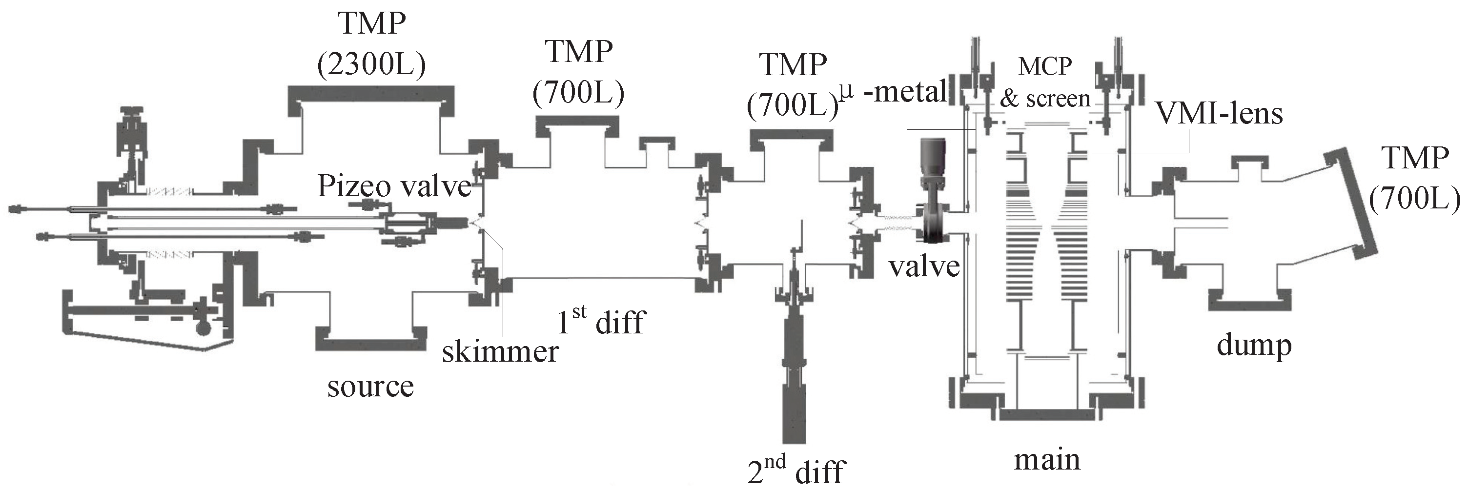
2. Apparatus
3. Simulation
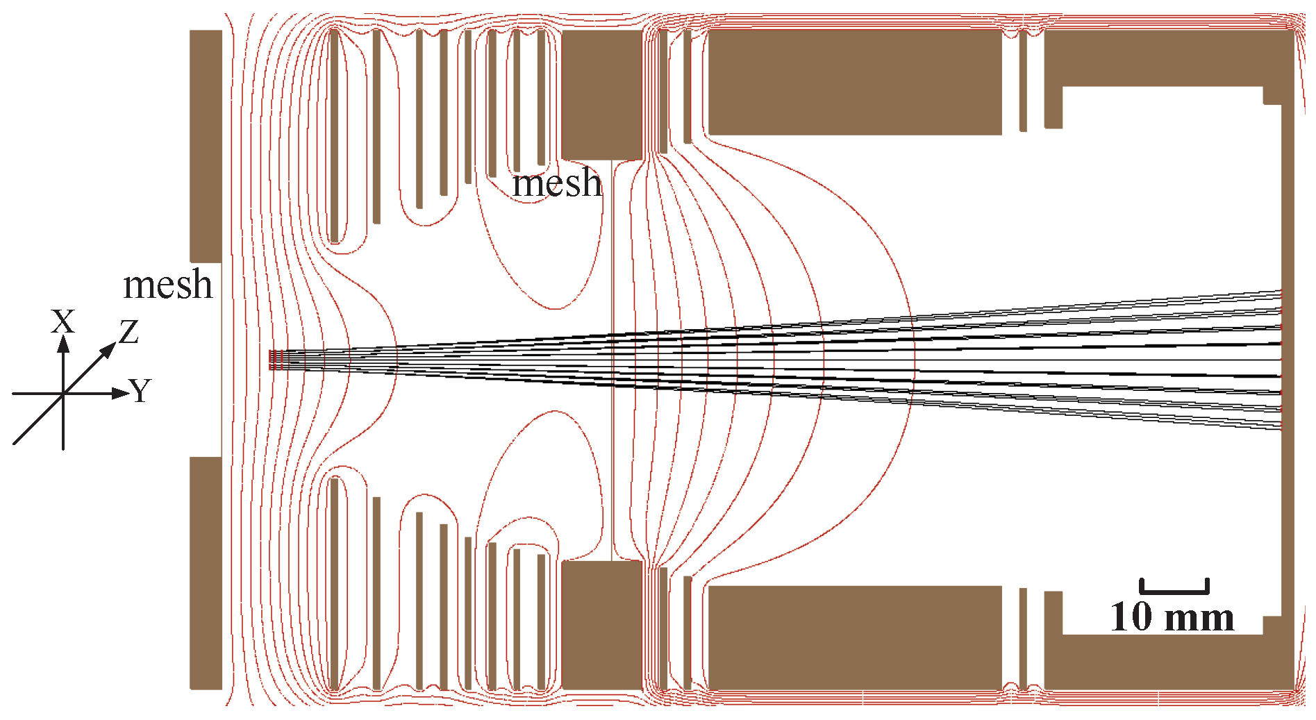
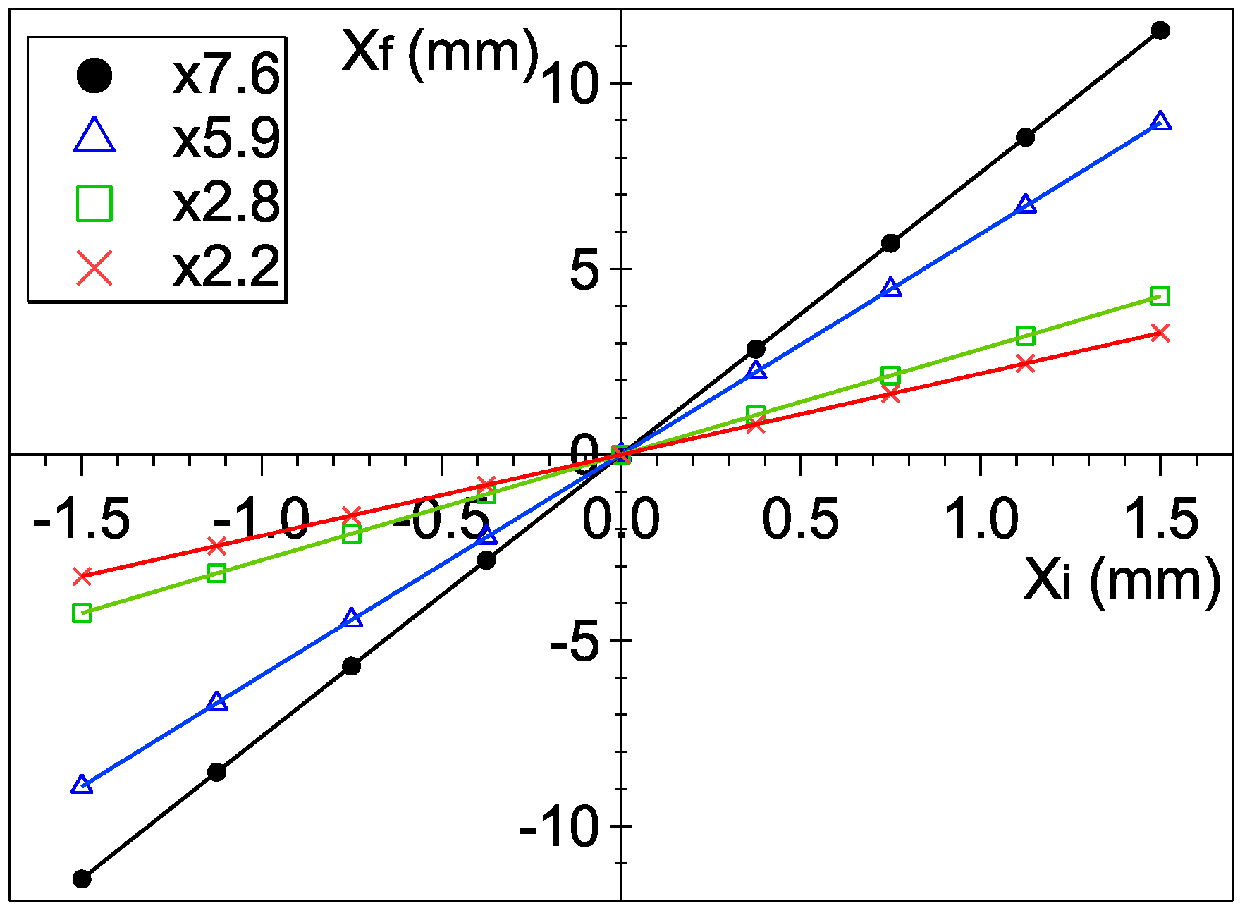
3.1. Spatial Mapping Mode
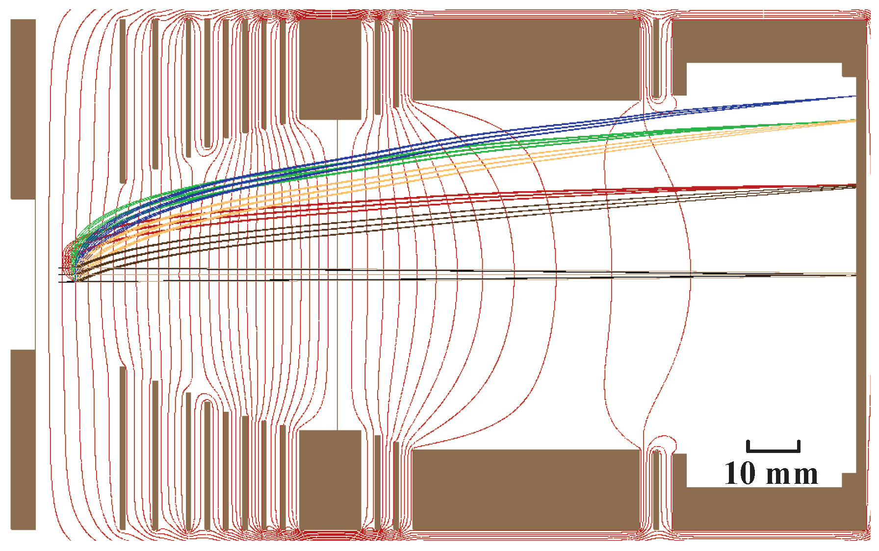
3.2. High-Resolution Momentum Mapping Mode
4. Experiment
4.1. Spatial Mapping Mode
4.2. High-Resolution Momentum Mapping Mode
5. Summary
Author Contributions
Funding
Institutional Review Board Statement
Informed Consent Statement
Data Availability Statement
Conflicts of Interest
References
- Chandler, D.W.; Houston, P.L. Two-dimensional imaging of state-selected photodissociation products detected by multiphoton ionization. J. Chem. Phys. 1987, 87, 1445–1447. [Google Scholar] [CrossRef]
- Eppink, A.T.J.B.; Parker, D.H. Velocity map imaging of ions and electrons using electrostatic lenses: Application in photoelectron and photofragment ion imaging of molecular oxygen. Rev. Sci. Instrum. 1997, 68, 3477–3484. [Google Scholar] [CrossRef]
- Garcia, G.A.; Nahon, L.; Harding, C.J.; Mikajlo, E.A.; Powis, I. A refocusing modified velocity map imaging electron/ion spectrometer adapted to synchrotron radiation studies. Rev. Sci. Instrum. 2005, 76, 053302. [Google Scholar] [CrossRef]
- Garcia, G.A.; Soldi-Lose, H.; Nahon, L. A versatile electron-ion coincidence spectrometer for photoelectron momentum imaging and threshold spectroscopy on mass selected ions using synchrotron radiation. Rev. Sci. Instrum. 2009, 80, 023102. [Google Scholar] [CrossRef]
- O’Keeffe, P.; Bolognesi, P.; Coreno, M.; Moise, A.; Richter, R.; Cautero, G.; Stebel, L.; Sergo, R.; Pravica, L.; Ovcharenko, Y.; et al. A photoelectron velocity map imaging spectrometer for experiments combining synchrotron and laser radiations. Rev. Sci. Instrum. 2011, 82, 033109. [Google Scholar] [CrossRef]
- Bodi, A.; Hemberger, P.; Gerber, T.; Sztáray, B. A new double imaging velocity focusing coincidence experiment: i2PEPICO. Rev. Sci. Instrum. 2012, 83, 083105. [Google Scholar] [CrossRef]
- Sztáray, B.; Voronova, K.; Torma, K.G.; Covert, K.J.; Bodi, A.; Hemberger, P.; Gerber, T.; Osborn, D.L. CRF-PEPICO: Double velocity map imaging photoelectron photoion coincidence spectroscopy for reaction kinetics studies. J. Chem. Phys. 2017, 147, 013944. [Google Scholar] [CrossRef] [PubMed]
- Rading, L.; Lahl, J.; Maclot, S.; Campi, F.; Coudert-Alteirac, H.; Oostenrijk, B.; Peschel, J.; Wikmark, H.; Rudawski, P.; Gisselbrecht, M.; et al. A Versatile Velocity Map Ion-Electron Covariance Imaging Spectrometer for High-Intensity XUV Experiments. Appl. Sci. 2018, 8, 998. [Google Scholar] [CrossRef]
- Cavanagh, S.J.; Gibson, S.T.; Gale, M.N.; Dedman, C.J.; Roberts, E.H.; Lewis, B.R. High-resolution velocity-map-imaging photoelectron spectroscopy of the O− photodetachment fine-structure transitions. Phys. Rev. A 2007, 76, 052708. [Google Scholar] [CrossRef]
- Kling, N.G.; Paul, D.; Gura, A.; Laurent, G.; De, S.; Li, H.; Wang, Z.; Ahn, B.; Kim, C.H.; Kim, T.K.; et al. Thick-lens velocity-map imaging spectrometer with high resolution for high-energy charged particles. J. Instrum. 2014, 9, P05005. [Google Scholar] [CrossRef]
- Ding, B.; Xu, W.; Wu, R.; Feng, Y.; Tian, L.; Li, X.; Huang, J.; Liu, Z.; Liu, X. A Composite Velocity Map Imaging Spectrometer for Ions and 1 keV Electrons at the Shanghai Soft X-ray Free-Electron Laser. Appl. Sci. 2021, 11, 10272. [Google Scholar] [CrossRef]
- Glownia, J.M.; Cryan, J.; Andreasson, J.; Belkacem, A.; Berrah, N.; Blaga, C.I.; Bostedt, C.; Bozek, J.; DiMauro, L.F.; Fang, L.; et al. Time-resolved pump-probe experiments at the LCLS. Opt. Express 2010, 18, 17620–17630. [Google Scholar] [CrossRef] [PubMed]
- Krausz, F.; Ivanov, M. Attosecond physics. Rev. Mod. Phys. 2009, 81, 163–234. [Google Scholar] [CrossRef]
- Lépine, F.; Ivanov, M.Y.; Vrakking, M.J.J. Attosecond molecular dynamics: Fact or fiction? Nat. Photonics 2014, 8, 195–204. [Google Scholar] [CrossRef]
- Erk, B.; Boll, R.; Trippel, S.; Anielski, D.; Foucar, L.; Rudek, B.; Epp, S.W.; Coffee, R.; Carron, S.; Schorb, S.; et al. Imaging charge transfer in iodomethane upon x-ray photoabsorption. Science 2014, 345, 288–291. [Google Scholar] [CrossRef]
- Allum, F.; Anders, N.; Brouard, M.; Bucksbaum, P.; Burt, M.; Downes-Ward, B.; Grundmann, S.; Harries, J.; Ishimura, Y.; Iwayama, H.; et al. Multi-channel photodissociation and XUV-induced charge transfer dynamics in strong-field-ionized methyl iodide studied with time-resolved recoil-frame covariance imaging. Faraday Discuss. 2021, 228, 571–596. [Google Scholar] [CrossRef]
- Corrales, M.E.; González-Vázquez, J.; Balerdi, G.; Solá, I.R.; de Nalda, R.; Bañares, L. Control of ultrafast molecular photodissociation by laser-field-induced potentials. Nat. Chem. 2014, 6, 785–790. [Google Scholar] [CrossRef]
- Corrales, M.E.; de Nalda, R.; Bañares, L. Strong laser field control of fragment spatial distributions from a photodissociation reaction. Nat. Commun. 2017, 8, 1345. [Google Scholar] [CrossRef]
- Johnsson, P.; Rouzée, A.; Siu, W.; Huismans, Y.; Lépine, F.; Marchenko, T.; Düsterer, S.; Tavella, F.; Stojanovic, N.; Redlin, H.; et al. Characterization of a two-color pump–probe setup at FLASH using a velocity map imaging spectrometer. Opt. Lett. 2010, 35, 4163–4165. [Google Scholar] [CrossRef]
- Benis, E.P.; Xia, J.F.; Tong, X.M.; Faheem, M.; Zamkov, M.; Shan, B.; Richard, P.; Chang, Z. Ionization suppression of Cl2 molecules in intense laser fields. Phys. Rev. A 2004, 70, 025401. [Google Scholar] [CrossRef]
- Tsatrafyllis, N.; Bergues, B.; Schröder, H.; Veisz, L.; Skantzakis, E.; Gray, D.; Bodi, B.; Kuhn, S.; Tsakiris, G.D.; Charalambidis, D.; et al. The ion microscope as a tool for quantitative measurements in the extreme ultraviolet. Sci. Rep. 2016, 6, 21556. [Google Scholar] [CrossRef]
- Stei, M.; von Vangerow, J.; Otto, R.; Kelkar, A.H.; Carrascosa, E.; Best, T.; Wester, R. High resolution spatial map imaging of a gaseous target. J. Chem. Phys. 2013, 138, 214201. [Google Scholar] [CrossRef]
- Bastian, B.; Asmussen, J.D.; Ben Ltaief, L.; Czasch, A.; Jones, N.C.; Hoffmann, S.V.; Pedersen, H.B.; Mudrich, M. A new endstation for extreme-ultraviolet spectroscopy of free clusters and nanodroplets. Rev. Sci. Instrum. 2022, 93, 075110. [Google Scholar] [CrossRef]
- Irimia, D.; Dobrikov, D.; Kortekaas, R.; Voet, H.; van den Ende, D.A.; Groen, W.A.; Janssen, M.H.M. A short pulse (7 μs FWHM) and high repetition rate (dc-5kHz) cantilever piezovalve for pulsed atomic and molecular beams. Rev. Sci. Instrum. 2009, 80, 113303. [Google Scholar] [CrossRef] [PubMed]
- Jones, W.; Clark, J. Simion Ion Optics Simulation. Ver 8.2. Available online: https://simion.com/ (accessed on 3 February 2024).
- Bergmann, T.; Martin, T.P.; Schaber, H. High-resolution time-of-flight mass spectrometers: Part I. Effects of field distortions in the vicinity of wire meshes. Rev. Sci. Instrum. 1989, 60, 347–349. [Google Scholar] [CrossRef]
- Peters, R.A. A new algorithm for image noise reduction using mathematical morphology. IEEE Trans. Image Process. 1995, 4, 554–568. [Google Scholar] [CrossRef] [PubMed]
- Radcliffe, P.; Düsterer, S.; Azima, A.; Li, W.B.; Plönjes, E.; Redlin, H.; Feldhaus, J.; Nicolosi, P.; Poletto, L.; Dardis, J.; et al. An experiment for two-color photoionization using high intensity extreme-UV free electron and near-IR laser pulses. Phys. Res. Sect. A Accel. Spectrometers Detect. Assoc. Equip. 2007, 583, 516–525. [Google Scholar] [CrossRef]
- Werby, N.; Natan, A.; Forbes, R.; Bucksbaum, P.H. Disentangling the subcycle electron momentum spectrum in strong-field ionization. Phys. Rev. Res. 2021, 3, 023065. [Google Scholar] [CrossRef]
- Zipp, L.J.; Natan, A.; Bucksbaum, P.H. Probing electron delays in above-threshold ionization. Optica 2014, 1, 361–364. [Google Scholar] [CrossRef]
- Roberts, G.M.; Nixon, J.L.; Lecointre, J.; Wrede, E.; Verlet, J.R.R. Toward real-time charged-particle image reconstruction using polar onion-peeling. Rev. Sci. Instrum. 2009, 80, 053104. [Google Scholar] [CrossRef]
- Nandor, M.J.; Walker, M.A.; Woerkom, L.D.V. Angular distributions of high-intensity ATI and the onset of the plateau. J. Phys. B At. Mol. Opt. Phys. 1998, 31, 4617. [Google Scholar] [CrossRef]
- León, I.; Yang, Z.; Liu, H.T.; Wang, L.S. The design and construction of a high-resolution velocity-map imaging apparatus for photoelectron spectroscopy studies of size-selected clusters. Rev. Sci. Instrum. 2014, 85, 083106. [Google Scholar] [CrossRef]
- Schomas, D.; Rendler, N.; Krull, J.; Richter, R.; Mudrich, M. A compact design for velocity-map imaging of energetic electrons and ions. J. Chem. Phys. 2017, 147, 013942. [Google Scholar] [CrossRef]
- Ghafur, O.; Siu, W.; Johnsson, P.; Kling, M.F.; Drescher, M.; Vrakking, M.J.J. A velocity map imaging detector with an integrated gas injection system. Rev. Sci. Instrum. 2009, 80, 033110. [Google Scholar] [CrossRef] [PubMed]
- Ablikim, U.; Bomme, C.; Osipov, T.; Xiong, H.; Obaid, R.; Bilodeau, R.C.; Kling, N.G.; Dumitriu, I.; Augustin, S.; Pathak, S.; et al. A coincidence velocity map imaging spectrometer for ions and high-energy electrons to study inner-shell photoionization of gas-phase molecules. Rev. Sci. Instrum. 2019, 90, 055103. [Google Scholar] [CrossRef]
- Skruszewicz, S.; Passig, J.; Przystawik, A.; Truong, N.X.; Köther, M.; Tiggesbäumker, J.; Meiwes-Broer, K.H. A new design for imaging of fast energetic electrons. Int. J. Mass Spectrom. 2014, 365–366, 338–342. [Google Scholar] [CrossRef]
- Goulielmakis, E.; Uiberacker, M.; Kienberger, R.; Baltuska, A.; Yakovlev, V.; Scrinzi, A.; Westerwalbesloh, T.; Kleineberg, U.; Heinzmann, U.; Drescher, M.; et al. Direct Measurement of Light Waves. Science 2004, 305, 1267–1269. [Google Scholar] [CrossRef] [PubMed]
- Isinger, M.; Squibb, R.J.; Busto, D.; Zhong, S.; Harth, A.; Kroon, D.; Nandi, S.; Arnold, C.L.; Miranda, M.; Dahlström, J.M.; et al. Photoionization in the time and frequency domain. Science 2017, 358, 893–896. [Google Scholar] [CrossRef]
- Vrakking, M.J.J. Attosecond imaging. Phys. Chem. Chem. Phys. 2014, 16, 2775–2789. [Google Scholar] [CrossRef] [PubMed]


| Geometry (mm) | Voltages (V) | ||||||||
|---|---|---|---|---|---|---|---|---|---|
| DIST | TH | ID | Ion | Electron | |||||
| ×1.0 | ×2.2 | ×2.8 | ×5.9 | ×7.6 | 150 eV | ||||
| 1 | −9 | 5 | 32 | 0.00 | 0.00 | 0.00 | 0.00 | 0.00 | 0.00 |
| 2 | 9 | 1 | 39 | −145.00 | −557.84 | −609.25 | −924.02 | −1026.46 | 710.86 |
| 3 | 16 | 1 | 45 | −215.00 | −630.63 | −655.37 | −806.86 | −856.11 | 1167.22 |
| 4 | 23 | 1 | 50 | −285.00 | −713.68 | −717.52 | −741.05 | −748.71 | 1690.25 |
| 5 | 27 | 1 | 54 | −325.00 | −725.84 | −725.75 | −725.23 | −725.05 | 1393.81 |
| 6 | 31 | 1 | 58 | −365.00 | −856.60 | −856.23 | −853.94 | −853.19 | 1749.89 |
| 7 | 35 | 1 | 60 | −405.00 | −1010.42 | −1010.02 | −1007.51 | −1006.70 | 2177.87 |
| 8 | 39 | 1 | 62 | −445.00 | −1102.81 | −1102.72 | −1102.10 | −1101.91 | 2725.96 |
| 9 | 43 | 1 | 64 | −485.00 | −1032.90 | −1147.87 | −1147.70 | −1147.65 | 3096.81 |
| 10 | 47 | 13 | 66 | −620.00 | −1147.79 | −1163.66 | −948.53 | −878.58 | 3583.11 |
| 11 | 63 | 1 | 68 | −685.00 | −1393.94 | −1394.95 | −1401.18 | −1403.20 | 3309.72 |
| 12 | 67 | 1 | 71 | −725.00 | −1499.74 | −1500.63 | −1506.08 | −1507.85 | 2819.75 |
| 13 | 71 | 48 | 74 | −1000.00 | −1610.91 | −1614.94 | −1639.63 | −1647.65 | 2282.31 |
| 14 | 122 | 1 | 75 | −1275.00 | −1636.33 | −1636.31 | −1636.18 | −1636.14 | 1654.07 |
| 15 | 126 | 41 | 76 | −1525.00 | −1715.00 | −1710.33 | −1692.93 | −1687.27 | 2000.00 |
| Author | Magnification Factor | Type |
|---|---|---|
| Tsatrafyllis [21] | 80.0 | Ion microscope |
| Stei [22] | −14.6 | Ion microscope |
| Benis [20] | 6.8 | Ion microscope |
| Johnsson [19] | −6.0 | Two-mode VMI |
| This work | 1.0, 1.5, 1.8, 5.2, 6.4 | Two-mode VMI |
| Author | KE [eV] | ΔE/E | Mesh | Year |
|---|---|---|---|---|
| Cavanagh [9] | 0.87 | 0.38% | NO | 2007 |
| León [33] | 3 | 0.53% | NO | 2014 |
| Kling [10] | 60 | 1.5% | NO | 2014 |
| Schomas [34] | 65 | 3.0% | NO | 2017 |
| Ghafur [35] | 100 | 1.8% | NO | 2009 |
| Ablikim [36] | 100 | 3.8% | NO | 2019 |
| Skruszweicz [37] | 300 | 4.0% | NO | 2014 |
| Ding [11] | 500 | 1.5% | YES | 2021 |
| This work | 44.6 | 1.3% | YES | 2023 |
Disclaimer/Publisher’s Note: The statements, opinions and data contained in all publications are solely those of the individual author(s) and contributor(s) and not of MDPI and/or the editor(s). MDPI and/or the editor(s) disclaim responsibility for any injury to people or property resulting from any ideas, methods, instructions or products referred to in the content. |
© 2024 by the authors. Licensee MDPI, Basel, Switzerland. This article is an open access article distributed under the terms and conditions of the Creative Commons Attribution (CC BY) license (https://creativecommons.org/licenses/by/4.0/).
Share and Cite
Feng, Y.; Ding, B.; Wu, R.; Jin, X.; Wu, K.; Liao, J.; Huang, J.; Liu, X. Spatial and Momentum Mapping Modes for Velocity Map Imaging Spectrometer. Appl. Sci. 2024, 14, 2190. https://doi.org/10.3390/app14052190
Feng Y, Ding B, Wu R, Jin X, Wu K, Liao J, Huang J, Liu X. Spatial and Momentum Mapping Modes for Velocity Map Imaging Spectrometer. Applied Sciences. 2024; 14(5):2190. https://doi.org/10.3390/app14052190
Chicago/Turabian StyleFeng, Yunfei, Bocheng Ding, Ruichang Wu, Xin Jin, Kefei Wu, Jianfeng Liao, Jianye Huang, and Xiaojing Liu. 2024. "Spatial and Momentum Mapping Modes for Velocity Map Imaging Spectrometer" Applied Sciences 14, no. 5: 2190. https://doi.org/10.3390/app14052190