Article

Multi-Objective Optimization of Cyclone Separators Based on Geometrical Parameters for Performance Enhancement

1
Department of Mechanical Engineering, Birla Institute of Technology, Mesra, Ranchi 835215, India
2
Faculty of Production Engineering and Logistics, Opole University of Technology, 76 Proszkowska St., 45-758 Opole, Poland
3
Faculty of Engineering and Applied Sciences, Usha Martin University, Ranchi 835103, India
*
Author to whom correspondence should be addressed.
Appl. Sci. 2024, 14(5), 2034; https://doi.org/10.3390/app14052034
Submission received: 3 January 2024 / Revised: 23 February 2024 / Accepted: 26 February 2024 / Published: 29 February 2024

Abstract

:
The present study focuses on performing multi-objective optimization of the cyclone separator geometry to lower the pressure losses and enhance the collection efficiency. For this, six geometrical entities, such as the main body diameter of the cyclone, the vortex finder diameter and its insertion length, the cone tip diameter, and the height of the cylindrical and conical segment, have been accounted for optimization, and the Muschelknautz method of modeling has been used as an objective function for genetic algorithms. To date, this is one of the most popular mathematical models that accurately predicts the cyclone performance, such as the pressure drop and cut-off particle size. Three cases have been selected from the Pareto fronts, and the cyclone performance is calculated using advanced closure large-eddy simulation—the results are then compared to the baseline model to evaluate the relative improvement. It has been observed that in one of the models, with merely a 2% reduction in the collection efficiency and an increase of 12% in the cut-off particle size, more than a 43% reduction in pressure drop value was obtained (an energy-efficient model). In another model, a nearly 25% increment in the collection efficiency and a reduction of 42% in the cut-off particle size with a nearly 36% increase in pressure drop value were observed (a high-efficiency model).

1. Introduction

The tremendous growth rate of the human population, followed by the modern lifestyle and work culture, has increased the demand for readymade products in day-to-day life, including eatables. This has led to a greater dependency on industrial products, due to which the demand for industries has increased. Furthermore, the rise in industries also contributes significantly to the economic growth and scientific advancement of a nation. However, this progress has a significant impact on the environment, particularly in terms of water and air pollution—the latter is of concern in the present study. Particulate matter (PM), which includes substances with aerodynamic diameters equal to or less than 10 and 2.5 µm, has emerged as a major concern and has been linked to well-known problems related to the respiratory system and disease in humans [1]. There is a strong correlation between exposure to PM10 and PM2.5, which are suspended in the air, and their harmful effects on health. Even at low levels, air pollution has detrimental health consequences both in the short and long terms [2,3,4,5]. Many industries are implementing pollution control equipment to collect these particles. Among all the equipment, cyclone separators are a popular choice due to their simple design and low maintenance requirements. However, these separators are inefficient for particles below 5 μm in size. Hence, the present study is aimed at enhancing the cyclone performance.
Several approaches have been attempted to improve the cyclone performance by modifying the standard geometrical parameters using different methods. Wasilewski and Brar [6] optimized the geometrical parameters for low power consumption with increased collection capabilities of the clinker-burning process. Luciano et al. [7] used a multi-objective optimization approach on cyclones arranged in series to improve efficiency. Singh et al. [8] optimized the Strokes number through the surrogate-based optimization. Sabareesh and Prasad [9] optimized various geometrical parameters of the Stairmand cyclone design utilizing response surface methodology. Pishbin and Moghiman [10] made use of genetic algorithms and numerical simulations and optimized the cyclone geometry for better performance. The authors found that the optimized cyclone design had a higher efficiency and lower pressure drop compared to the original design. The study also showed that the genetic algorithm was an effective tool for optimizing the cyclone separators. An innovative method for advancing centrifugal treatment equipment involves integrating dusty flow filtration with centrifugal cleaning [11,12,13,14]. Many researchers have extensively investigated these innovations, with particular emphasis on exploring new-generation multi-channel cyclones, as highlighted by [15,16,17]. Baltrenas and Chlebnikovas [18] applied multi-channel cyclones and observed that the purification efficiency from fine wood ash solid particles reached 83.6% after 150 h of operation. Jurevicius [19] examined common tendencies in the sticking process of particles of various sizes and proposed a model suitable for numerically simulating ultrafine particle interactions. The cyclone performance was reported to have significant variations by Parvaz et al. [20], who examined the effect of providing a 4–10% eccentricity to the vortex finder. In a related study, the authors analyzed various shapes of the dipleg and found that the inverted cone dipleg exhibited superior separation capability compared to the standard model [21]. Similarly, Sun et al. [22] also employed optimization techniques to improve the performance of the cyclone separators by optimizing geometry and inlet configuration, leading to increased particle collection efficiency and reduced pressure drop.
Brar and Elsayed [23] conducted a study involving multi-objective optimization on the positioning and size of secondary inlets—they reported tremendous improvement compared to the reference model. Guo et al. [24] conducted optimization-based work on the slotted vortex finder (SVF). Their study resulted in a 34.57% reduction in the Euler number and a 4.32% enhancement in the collection efficiency, followed by a reduction of nearly 5.53% in the cut-off diameter. In a similar study, Elsayed et al. [25] optimized the length, height, and diameter of the dustbin, achieving superior performance over the baseline model. Furthermore, Kumar and Jha [26] were able to attain better results compared to the reference geometry via optimization of the convergent–divergent outlet tube. Brar and Elsayed [27] carried out multi-objective optimization with an artificial neural network (ANN) as well as the genetic algorithm (GA), which resulted in considerably minimum pressure drop and maximum collection efficiency over different (eccentric) locations of the vortex finder centers. Shastri et al. [28] carried out multi-objective optimization using the Muschelknautz method of modeling (MM) to optimize the cyclone performance for a fixed total height condition. The study considered three optimization scenarios, and a noteworthy improvement in cyclone models was reported.
To date, the Muschelknautz method of modeling (MM) [29,30] has become one of the most widely used mathematical models. This is due to only a few simplifying assumptions, the incorporation of all the geometric entities, the consideration of the fluid contraction at the inlet, the mass loading effects of the solid particles on the cyclone performance, the impact on the frictional drag due to total inside area of the separator, etc. Because of this, the MM model has been extensively used in the current work. This model can predict the cut-off size and pressure losses with a high level of accuracy in nearly all cyclone designs [14].
Most of the studies undertaken so far did not include the cyclone main body diameter for optimization. This parameter significantly influences the pressure drop values and moderately affects the collection efficiency. With an increase in the cyclone diameter, there is an increase in the pressure drop, whereas the collection efficiency reduces by a small amount. In the latter, the efficiency of bigger particles largely increases, whereas for smaller particles, the efficiency mildly reduces, as reported by Brar and Sharma [31]. Hence, the cyclone diameter is worth considering for optimization. Shastri et al. [28] accounted for this parameter in an optimization study, and the results showed significant improvement over the reference model—the authors focused on compact cyclone separators, for which they chose to fix the total height of the cyclone. It is also known that an increase in the cyclone length tremendously reduces the pressure losses, followed by a significant increase in the collection efficiency. Brar et al. [32] reported a 34% reduction in pressure losses and a nearly 10% increase in collection efficiency for elongation in the length of the cylindrical segment from 1.5 to 5.5 times the cyclone diameter. On the other hand, increasing the cone length from 2.5 to 6.5 times the cyclone diameter resulted in an 11% increase in efficiency, whereas the pressure losses reduced by 29%.
Based on the above discussion, it follows that both the cyclone’s main body diameter and total height must also be included for optimization. However, most of the studies have neglected the main body diameter of the cyclones for optimization. Hence, in the present study, all the geometrical entities are considered for optimization to reduce both the pressure losses and cut-off particle size. For this, we make use of the expressions from the MM as objective functions subjected to optimization using Ga with the prescribed range for all the independent variables. Hence, the work has been planned in the following manner: Firstly, the flow system has been defined with detailed information on cyclone geometry. Then, we elaborate on the MM, followed by the description of the range by which each independent geometrical entity is permitted to vary. Thereafter, the objective function is subjected to optimization using Ga to yield the Pareto front (or optimal) points. The selected Pareto front points are then numerically simulated using the advanced closure large-eddy simulation for cross-validation and to explore the flow field details. Finally, the performance level of the (chosen) optimized cyclones is compared to the baseline model to evaluate the relative enhancement in the performance parameter.

2. Mathematical Modeling

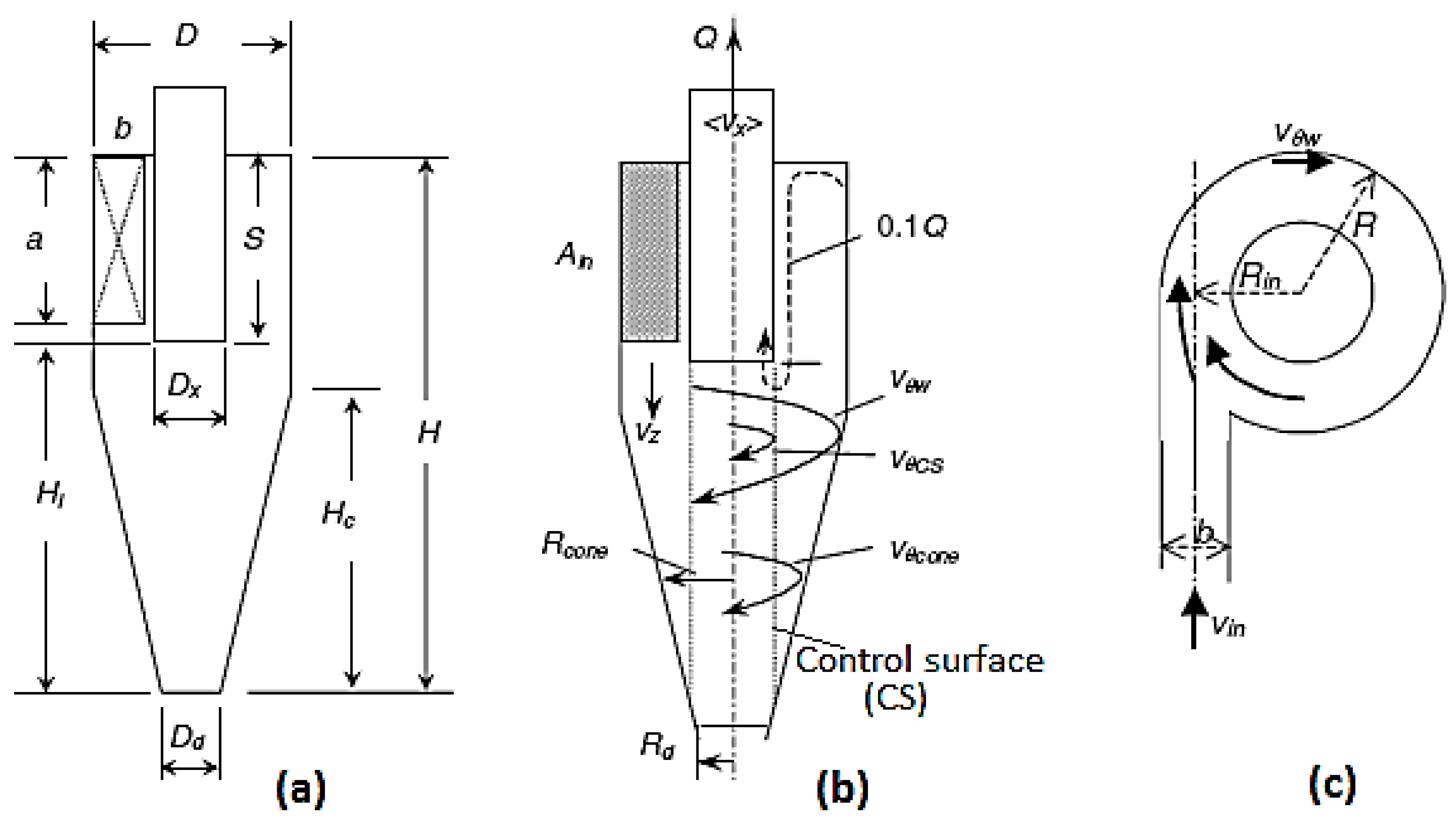
2.1. The Geometric Details

The baseline model in the current work is the design suggested by Stairmand [33]—the geometry is the cylinder-on-cone model with a tangential inlet. As shown in Figure 1, the geometrical entities include the vortex finder diameter, De/D = 0.5, and its insertion length, Lv/D = 0.5; the inlet height, a/D = 0.5, and width, b/D = 0.2; the cylinder height, H/D = 1.5; the cone height, Hc/D = 2.5; and the cone tip diameter, Bc/D = 0.375. The diameter of the cyclone D = 0.29 m. Although the original diameter of the cyclone is represented as D, we also designate it as Dc, and it shall represent the new optimized diameter. It is important to mention here that Dc is also normalized with the original diameter D, similar to all other geometrical entities.

2.2. Muschelknautz Model

So far, numerous analytical models have been developed to determine the performance of the cyclone. The Muschelknautz model is the most popular and the most efficient model to determine the collection efficiency and pressure drop [34]. This model accounts for the following:
(a)
The wall roughness.
(b)
The variation in the feed of the particle size distribution.
(c)
The solid particle loading.
Muschelknautz and Trefz [29] further reported that the short-circuit flow causes 10% of the fluid entering the cyclone to escape directly through the vortex finder tube, while 90% remains in the cyclone body. By utilizing the empirical formulas relating the gas friction factor to the Reynolds number of the cyclone body, it is possible to approximate the friction factors for the gas and the particles. They further demonstrated that the density of strands of solids along the cyclone walls also contributes to increased friction.

2.2.1. Prediction of the Pressure Drop

The pressure drop across the cyclone occurs mainly due to friction between the fluid and the walls, irreversible losses within the vortex core, and inlet acceleration losses. The latter often dominates the total pressure drop. The losses developed inside the body are determined by the following:
  P b o d y = f A R 0.9 Q ρ 2 ( ν θ w ν θ c s ) 1.5
where f denotes the friction factor, ρ represents the gas density, the volume flow rate is given by Q, ν θ w is the velocity at the wall, ν θ c s is the tangential velocity of the rotating fluid in the inner core radius, and AR represents the total inside surface area (contributing to the frictional drag).
The pressure drop in the inner surface of the outlet tube is given as follows:
P c = 2 + v θ c s v c 2 + 3 v θ c s v c 4 / 3 1 2 ρ v c 2
where v c is the average axial velocity of the gas exiting via the vortex finder. Hence, the total pressure loss,
  P t o t a l =   P b o d y + P c
In non-dimensional form, the above expression is written as follows:
E u = 1 1 2 ρ v i n 2 (   P b o d y + P c )      
Here, Eu denotes Euler’s number, and the gas velocity at the inlet is vin.

2.2.2. Prediction of the Cut-Off Size

Given the solid loading to be sufficiently low, the cut-off particle size is given as follows:
  x 50 = 18 μ ( 0.9 Q ) 2 π   ( ρ p ρ ) ν 2 θ c s ( H t S )  
ρ p represents the density of the particulate phase. Moreover, the fluid viscosity is represented as µ, the cyclone length is designated by Ht, and S is the insertion depth of the outlet tube. For further information on the MM, we refer to Hoffmann and Stein [34], and the details are mentioned in Appendix A.

2.3. Genetic Algorithms

The genetic algorithm is an algorithm for resolving both limited and unconstrained optimization issues. It is based on natural selection, which promotes biological evolution. The genetic algorithm chooses members of the present population to serve as parents at each stage and employs them to produce the offspring that will make up the following generation. The population “evolves” toward the best option (here, the MM has been considered) over the course of subsequent generations until the optimum solution is reached. The genetic algorithm is used to address a range of optimization problems, including those where the objective function is discontinuous, stochastic, or highly nonlinear. Here, the MM of modeling has been used to evaluate the fitness of the individuals. The objective will be to minimize the pressure losses as well as the cut-off particle size. Table 1 shows the upper and lower bounds of the geometry used to optimize the cyclones, and Table 2 illustrates the settings adopted for Ga.

2.4. Computational Fluid Dynamics

The performance of a few chosen Pareto front points and the standard model are assessed and compared in the current study using CFD. The cost of the experimental setup is significantly reduced because of the well-established and extensively used CFD technique. The numerical predictions are as accurate as experimental findings when used appropriately with the prescribed boundary conditions, and by employing a suitable turbulence model—for the latter, we use the advanced closure LES.

2.4.1. Continuous Phase

Large Eddy Simulation

The LES adopts a filtering approach to distinguish between large and small eddies, with the filter function which is represented as [35] follows:
ϕ ¯ x = D ϕ ¯ x   G ( x , x ) d x
The integration over the flow domain (D) through the computational grid is represented as
ϕ ¯ x = 1 V υ ϕ x   d x , x  
where V represents the volume of the computational cell. The filter function is given as follows:
G x , x = 1 V , x υ   0 , x   o t h e r w i s e
The application of filtering on Navier-Stokes equations yields the following:
u i ¯ x i = 0
u i ¯ t + u j ¯ u i ¯ x j = 1 ρ P ¯ x i + υ 2 u i ¯ x i x j T i j x j
The over-bar is used to represent the filtering quantity. The subgrid-scale Reynolds stress, T i j = u i ¯   u j ¯ u i ¯ u j ¯ is modeled using the Boussinesq hypothesis as follows:
T i j 1 3 τ k k δ i j = 2 μ s g s S ¯ i j
where µsgs represents the sub-grid scale viscosity. The strain rate in the resolved flow is given as follows:
  S ¯ i j = 1 2 u i x j + u j x i

Modeling the Particulate Phase
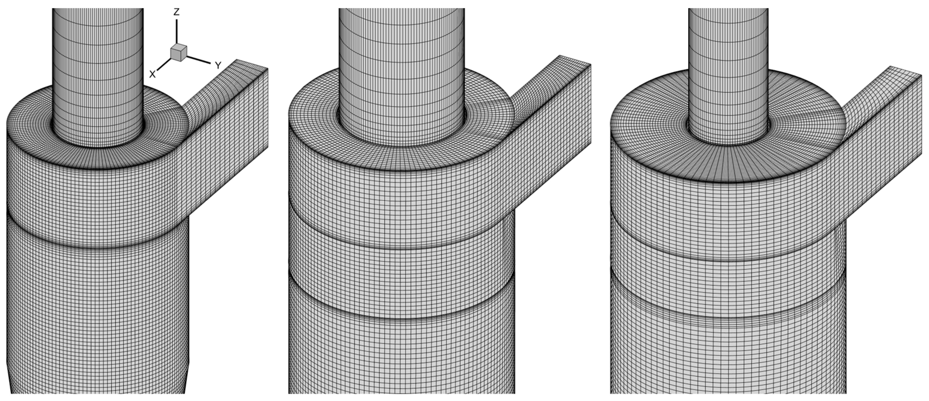
For a discrete particle traveling in a continuous fluid medium, the net force acting on the particles is calculated using Newton’s second law [36]:
d u p i d t = F D   u i   u p i +   ρ p ρ   ρ p   g i +   F i
Here, the density of the discrete phase is given as   ρ p , F D   u i   u p i represents the drag force on each particle per unit mass (here, i represents the flow direction),   u p i is the particle’s velocity,   g i is the acceleration due to gravity,   F i represents the additional forces (e.g., the Saffman lift force, Brownian force, etc.). For the spherical particles suspended in the fluid, the drag force is given as follows:
F D = 18 μ C d ρ p d p 2 · R e p 24
Here, particle diameter is denoted as dp, fluid molecular viscosity as µ, and Rep is the Reynolds number of the particle, given as follows:
R e p = ρ d p   u p i   u i μ
The drag on smooth particles is due to Morsi and Alexander [37], given as follows:
C D = a 1 + a 2 R e p + a 3 R e p 2
where the coefficients a 1 , a 2 , and a 3 are constants.
The instantaneous velocity for the fluid flow is expressed as u i = u ¯ i + u i ; where u i represents the instantaneous velocity, u ¯ i is the mean velocity component, and u i is the fluctuating velocity component. Since the LES works on the filtering approach, the directly resolved LES field very much resembles u i (same as used in Equation (13)), thereby requiring no approximation to account for the particle dispersion due to velocity fluctuations. However, for the unresolved part of the flow, stochastic modeling is required to be introduced using the discrete random walk (DRW) model—taken as discrete piecewise constant functions of time—and is given as follows:
u i = ζ 2 3 k
where ζ is a normal distributed random number and k is the sgs turbulent kinetic energy.

Meshing

The multi-block approach has been used, wherein the blocks are split to fill the entire domain with the industry-leading tool ICEM CFD. The grids obtained are non-orthogonal and fit well to the complex geometry. To minimize the effects of numerical diffusion, the cell faces are aligned in the direction of the fluid flow. The mesh closer to the boundaries and near the geometric axis is refined to capture the near-wall flow physics and impacts of the precessing vortex core near the geometrical axis, respectively. Figure 2 represents the details of the surface mesh of cyclones A, B, and C, consisting of 1.287 million, 1.092 million, and 1.114 million hexahedra, respectively. We have checked the results at two levels of the grid for all four models. The refinement (by more than 2.5 times that of the coarse mesh) was performed on a global basis, which also included further refinement of the grid at the boundaries at higher mesh counts. The maximum aspect ratio was around 68 at the conical walls of the refined mesh. When comparing the two levels of the grid, a maximum difference of 2.23% in pressure drop and 4.17% in the cut-off particle size was observed in cyclone model C. The results from the coarse mesh have only been presented.

Numerical Settings

The RNG k-ε turbulence model was initially used for the steady-state simulations until the residuals became (quasi-) steady with the number of iterations. The standard wall function was selected, and the solver tolerance was set at 10−5. This method significantly reduced the computational efforts, and the resulting flow field served as a starting point for LESs. The simulations were run till the monitored flow variables became stable with time. To couple the pressure and velocity, we use the NITA (Non-iterative Time Advancement) algorithm (in accordance with [38]), followed by the fractional step scheme. NITA utilizes more memory compared to the iterative time advancement technique, but it saves significant computational time. The pressure was discretized using the PRESTO! Interpolation scheme (as in [39]), which is optimized for the swirling flows with steep pressure gradients. For momentum, a bounded central differencing scheme was used, and for time enhancement, a bounded second-order implicit scheme was used.
Numerous spherical particles were ejected from the inlet plane inside the cyclone, and the collection efficiency was computed based on the particles escaping via the outlet boundary. Air is taken as the continuous phase that has a density of 1.2 kg/m3 and a viscosity of 2·10−5 kg/m·s. The inlet plane is subjected to the velocity inlet boundary condition, wherein a uniform velocity profile with Uin = 16.1 m/s was prescribed. The pressure outlet boundary condition has been used at the overflow plane. On all other boundaries, a no-slip boundary condition was applied. The sub-grid scales have been modeled using a Smagorinsky-Lilly model with a Smagorinsky constant CS of 0.1. For the near-wall treatment and damping function, we refer to Brar and Derksen [40]. Numerical simulations are performed with a time step size of 10−4 s on each of the tested models.
The discrete phase modeling (DPM) method, also known as the Euler-Lagrange method in conjunction with the continuous phase, was used to simulate the trajectories of solid particles. Particles with a density of 2700 kg/m3 and diameters ranging from 0.5 μm to 8 μm are employed for DPM. At the inlet of the cyclone, particulate matter having different diameters was introduced in a direction normal to the surface at a velocity similar to that of the fluid. The bottom plane is taken as the trap, so the solids reaching this plane are considered trapped, and their calculations are abolished from the fluid domain. Due to a very low solid loading condition, one-way coupling has been granted. The particle motion equation was discretized using the trapezoidal approach, and 900,000 integration steps were employed to trace the particle paths. A perfectly elastic collision between the discrete phase matter and the solid walls has been assumed. The particles touching the surface of the outlet tube were treated as an escape. Similar solver settings have been used in several studies [41,42,43,44,45,46,47,48,49,50].

Settings for the Genetic Algorithm

The optimization toolbox of MATLAB 2020 is utilized for the genetic algorithm for multi-objective optimization. The optimization process was carried out until a variation of less than 0.0001 for 100 consecutive iterations was observed. A similar setting was used earlier by numerous authors. The GA settings are elucidated in Table 2.

2.5. Validation

The CFD methodology must be verified against the available experimental data before using it for the analysis of the cyclones. In the present study, the results from the numerical simulations are compared to the experimental data of Hoekstra [51] at various axial locations, such as Z = 0.75D, 2.0D, and 2.5D. In the experiment, Hoekstra [51] considered the Stairmand high-efficiency cyclone with a diameter (D) equal to 0.29 m. A collection bin with a diameter of D and a height equal to 2.0D was installed at the bottom opening. An inlet velocity (Uin) equal to 16.1 m/s was used in the experiment that corresponds to the Reynolds number equal to 2.8 × 10⁵ (here, the Reynolds number is calculated as Re = ρ·Uin·D/µ, with ρ as the fluid density; Uin is the superficial inlet velocity at the inlet; D is the cyclone main body diameter; and µ is the fluid viscosity). The two levels of the grid have been tested here to evaluate the effect of cell counts on the results. The first level mesh (referred to as the coarse mesh) comprised 0.885 million hexahedra, whereas the second level mesh (referred to as the fine mesh) consisted of nearly 2.187 million hexahedra. Figure 3 shows the comparison between the two levels of the grid as well as with the reference data. It becomes apparent that at the two levels of the mesh, there is no appreciable change in the mean and root mean square error values at all the axial stations. Hence, the results may be considered grid independent. Furthermore, a very good agreement is observed between the numerically simulated results and the experimental data. The mean profile from the LES fits well with the reference data at each axial location. However, there is a mild overprediction in the mean tangential velocity profile as well as the rmse values of axial velocity (in the core region). To validate the discrete phase simulation methodology, we make use of the experimental data by Zhao [36], and the results are presented in the last row of Figure 3. Two levels of the mesh consisting of 1.21 and 2.45 million hexahedra were considered, which indicates that the results are grid-independent and that the simulation results fit well with the experimental data. Since the cyclonic flows are highly anisotropic and turbulent, validation can be accepted with a fair level of accuracy. Hence, the solver settings, as well as the boundary condition applied, are appropriate and can be used in all future simulations with confidence.

3. Results and Discussion

3.1. Pareto Front Points

As discussed earlier, for optimization, we make use of the equations from the MM as the fitness function in genetic algorithms. The objective here is to minimize the pressure losses as well as the cut-off particle size. Hence, the MM has been used to perform multi-objective optimization using MATLAB. The optimal data sets—also known as Pareto front points—have been presented in Figure 4. It becomes apparent that there is a trade-off between the two objective functions, such as the pressure drop and cut-off particle size. All the details have been presented in Table 3. Based on the relevance, three Pareto front points have been selected for analysis, namely A, B, and C. CFD analysis of these points has been carried out for cross-validation with GA predictions to quantify the performance with respect to the baseline (Std) model and to explore the flow field in detail (discussed next).

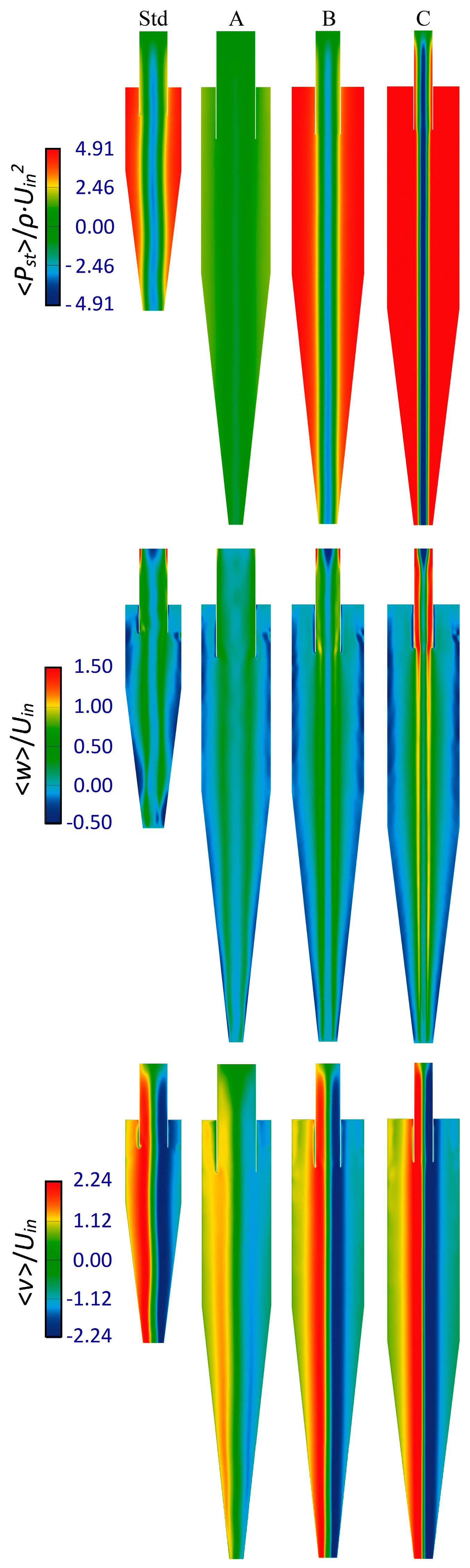
3.1.1. Mean Flow Field

The contour plots of the normalized mean static pressure, mean axial velocity, and mean tangential velocity of all the models are represented in the first, second, and third rows of Figure 5, respectively, and the corresponding radial profiles are represented in Figure 6. From the first row, it becomes apparent that the pattern of the pressure distribution is similar in all models—the pressure is at its maximum near the walls and lowest near the rotational axis of the inner core. This is due to the strong swirling nature of the flow. The mean pressure value is highest near the walls in model C and lowest in A, with a comparable value in Std as well as the B model that takes intermediate values. The same can be seen in the radial profiles at all the axial stations, such as z/D = 1.0, 2.0, and 3.0 (from left to right, respectively) in Figure 6. The magnitude of the pressure field relates to the pressure drop values—the greater the wall static pressure, the more pressure losses are expected. Near the geometrical axis, the lowest pressure is observed in model C and the highest in model A, with models B and Std having intermediate values. Large pressure gradients exist in the core region of model C, and this regime is very narrow. This contrasts with the pressure distribution in model A, where the (relative) variations are very few.
The second row in Figure 5 elucidates the contour plots of mean axial velocity, and the second row in Figure 6 represents its radial profiles at different axial stations. It becomes apparent that the axial velocity is directed in the downward direction near the solid walls (also termed the outer vortex region) and in the upward direction in the core region. The flow reversal takes place once the downwardly directed swirling flow touches the bottom plate of the cyclone. In the outer vortex region, the axial velocity magnitude is seemingly the same in all models. However, the difference is observed in the inner vortex regime—its magnitude is maximum in model C, followed by models B, Std, and A (in ascending order). The same is reflected in the radial profiles at all stations.
The last row in Figure 5 and Figure 6 represents the contour plots and radial profiles of mean tangential velocity, respectively. The tangential velocity magnitude is maximum in model C and lowest in model A, with intermediate values for Std and B models that have nearly similar values. Clear information is available in the radial profiles. The mean tangential velocity magnitude increases linearly in the core region till it reaches the outer region of the inner vortex. Thereafter, it reduces nonlinearly until it reaches the cyclone walls, where it takes the lowest value. The slope of the tangential velocity has the maximum values for model C, which indicates a much faster-rotating vortex core than other models. A minimum value is observed in model A, and its slope indicates the slowest rotation of the inner vortex. It is important to note that due to the high rotational rate of the inner vortex in model C, the dip in the static pressure profile is prominent, followed by the narrowest zone compared to the other models.

3.1.2. Fluctuating Flow Field

In cyclones, the inner vortex center does not coincide with the cyclone axis while it rotates. This rotating vortex undergoes lateral movements, adding to its precessing nature. The resulting phenomenon is referred to as the precessing vortex core (PVC) that causes significant enhancement in the levels of pressure and velocity fluctuations. These fluctuations are detrimental to the cyclone performance—collection efficiency, in particular—as they lead to the dispersion of the particles near the wall region. Hence, exploring the fluctuating field is of utmost importance, and in this study, it is represented by root mean square error (rmse) values that relate to the fluctuation levels of the velocity components.
As a common observation (cf. contour plots in Figure 7, and radial profiles in Figure 8) the pressure and velocity fluctuations are largest in the core region, referred to as the coherent fluctuations. In the outer region, these fluctuations do not have direct influence, so the nature of the fluctuations is turbulent—the latter is much weaker compared to the former. Cyclone model A exhibits the lowest level of fluctuations, while model C has the largest fluctuations of both the scalar and vector fields. Seemingly, the models Std and B have a nearly similar fluctuation level. The same observation, i.e., a high level of fluctuations in the core region, is apparent from the radial profiles. However, in the outer vortex regime, there are observable differences—the pressure fluctuations are reluctant, while for the axial and tangential velocities, many variations in the turbulent fluctuation levels are observed.

3.1.3. Vortex Core Representation

As mentioned earlier, the precessing frequency of the vortex core is a significant factor, typically influenced by the geometry of the cyclone and operating conditions [52]. Such vortical structures are best represented by the λ2 criterion and represented in Figure 9, which represents the iso-surface with a level set to 0.25. The vortex core is seemingly a twisted rope-like structure that extends throughout the cyclone length. Eddies with varying length scales can also be seen in the outer vortex region. Interestingly, in models B and C, the vortex core is seen to be surrounded by another (helical) vortex (resembling a snake wrap). The diameter of the vortex core reduces with an increase in the rotational speed.

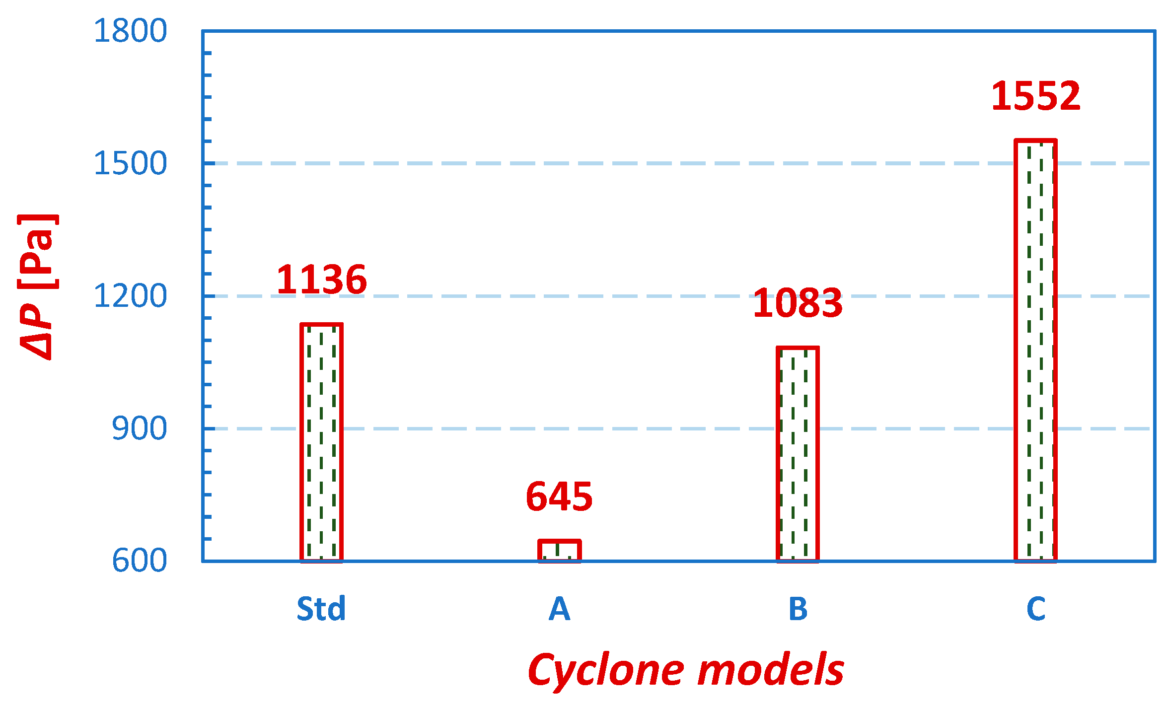
3.1.4. Cyclone Performance

In general, the performance of the cyclones is determined based on the pressure drop values (∆P), collection efficiencies (η), and cut-off diameters (d50). The pressure drop refers to the (total) pressure difference between the inlet and outlet, whereas the cut-off diameter is defined as the particle size corresponding to 50% collection efficiency on the grade efficiency curve (GEC). Separation efficiency denotes the ratio of particles retained by the cyclone separator to the injected particles at the inlet of the cyclone separator.
In cyclones, the pressure losses take place mainly inside the outlet tube due to the contraction experienced by the swirling fluid as well as wall friction. The pressure drop for all the models of the cyclones is presented in Figure 10. The maximum pressure drop was found in model C and lowest in model A, with the intermediate values for the model Std and B. This is due to the reduction in the diameter of the vortex finder, which significantly increases the magnitude of the tangential velocity. With respect to the Std model, the pressure drop in models A, B, and C increases by −43.22%, −4.67%, and 36.62%, respectively.
The GECs for all the models operating are presented in Figure 11. Compared to the Std model, a significant shifting of the curves toward the left takes place in models B and C, whereas model A gradually shifts toward the right. Figure 12a summarizes the d50 values for the different cyclone models. It is observed that the largest value of d50 exists for model A, while the smallest value is found for model C, with the intermediate value for model B. Compared to the Std model, d50 increases by 12.3%, −15.71%, and −41.94% in models A, B, and C, respectively. Figure 12b denotes the overall collection efficiency for all the models. It becomes apparent that model C has the highest value of η, whereas model A has the lowest value. Compared to the Std model, η increases by −2.16%, 19.05%, and 24.69% in models A, B, and C, respectively. The enhancement in η or reduction in d50 is due to the largest magnitude of the tangential velocity, which creates a strong centrifugal field that enhances the particle separation process.
Due to the change in the cyclone height, the cyclone volume changes significantly, which in turn influences the residence time (Tres) of particulate matter—here, Tres is the time for which the particles stay inside the cyclone. Figure 13 illustrates the Tres for all cyclone models (the calculations consider solids that exit the cyclone via the outlet plane). For all particle sizes, the Std model possesses the smallest Tres, whereas for all other models, variations in Tres are dramatic. Maximum value of Tres for particle sizes of 0.5, 1.0, 1.5, 2.0, 2.5, 4.0, 6.0, 8.0, and 10.0 µm is observed in cyclone models C, B, A, B, C, A, A, and A, respectively. A complete detail is provided in Figure 13. Interestingly, the solids having a size greater than 2.5 µm are collected with 100% efficiency. Hence, no particle greater than this size reaches the outlet plane, due to which their Tres values are zero.
The movement of solid particles at different realizations inside the body of cyclones A and B are represented in Figure 14. The strands of the solid particles are represented as a function of particle diameter. It can be seen that the solids of different diameters mix very well. The smaller particles start escaping at a very early stage, whereas the mid to large-ranged solid particles get closer to the outer wall and follow a definite pattern.

4. Conclusions

The objective of this study was to enhance the effectiveness of the Stairmand cyclone separator through the optimization of its geometry. The Muschelknautz method of modeling (MM)—a well-known mathematical model used for predicting pressure losses and cut-off diameter of the particulate phase—was utilized for optimization using genetic algorithms. All geometrical parameters, which include inlet dimensions, vortex finder diameter and its insertion length, cyclone main body diameter, cone tip diameter, and conical section height, were taken into consideration for optimization. A few cases from the Pareto front points were selected, and numerical simulations were performed using advanced closure LES to assess the relative performance with respect to the baseline model. The investigation defines the importance of considering the cyclone main body diameter (Dc/D) for optimization, and the optimized diameter was observed to take a larger value than the original size. Conclusive results indicate the following:
  • In cyclone model A, the pressure losses decreased significantly by 43.22%, with a marginal reduction of 2.16% in the overall collection efficiency and an increase in the cut-off size by 12.3%.
  • In model B, with a reduction in the pressure drop by 4.67%, cut-off sizes decreased by 15.71%, with a 19.05% enhancement in the collection efficiency.
  • In Model C, with an increase in the pressure drop by 36.62%, the cut-off size decreased by 41.94%, and the collection efficiency increased by 24.69%.
Overall, the results of the study imply that the optimized geometries were significantly better than the standard model regarding particle separation efficiency and pressure drop. The research underscores the importance of considering all geometrical parameters to achieve optimal performance in the cyclone separators. With the large number of optimized datasets provided in the manuscript, the designers will have a wide choice of appropriate ones to select. Since all the geometric entities are normalized with the original diameter of the cyclone, there is flexibility when applying them to any cyclone size. As an extension to the present study, the future plan is to also optimize the cyclone performance based on the particle loading condition.

Author Contributions

Conceptualization, L.S.B.; methodology, L.S.B.; software, S.P., L.S.B., A.M., O.P., A.A. and M.W.; validation, S.P. and M.W.; formal analysis, M.W.; A.M. and O.P. investigation, S.P., L.S.B. and M.W.; resources, S.P. and O.P.; data curation, S.P., L.S.B., A.M., O.P., A.A. and M.W.; writing—original draft preparation, S.P. and L.S.B.; writing—review and editing, S.P., L.S.B., A.M., O.P., A.A. and M.W.; visualization, S.P. and L.S.B.; supervision, L.S.B.; project administration, L.S.B. All authors have read and agreed to the published version of the manuscript.

Funding

This research received no external funding.

Data Availability Statement

The original contributions presented in the study are included in the article, further inquiries can be directed to the corresponding author.

Conflicts of Interest

The authors declare no conflict of interest.

Nomenclature

aheight of the cyclone inlet
Ainlet area of the cyclone
bwidth of the cyclone inlet
Bccone tip diameter of the cyclone
CDdrag force coefficient
CsSmagorinsky constant
dpparticle diameter
d50cut-off size
Ddiameter of the standard cyclone model/characteristic diameter
Dc(optimized) cyclone diameter
DL,ijmolecular diffusive transport term
DT,ijturbulent diffusive transport term
Dxvortex finder diameter
ffrequency of oscillation of the PVC
Fiadditional forces per unit mass
FDdrag force
ggravitational accelerations
Hclength of the cylindrical segment of the cyclone
kvon Kármán constant
lcharacteristic length
Lslength scale of subgrid-scales
Lv, Sinsertion length of the vortex finder diameter inside the cyclone
mpparticle mass
pinstantaneous gas static pressure
Pmean static pressure of the gas
p0pressure at the symmetric axis
p’fluctuating gas pressure
p ¯ resolved static pressure
Pdifferential pressure measurement
Pijstress generation term
Qthe volume flow rate of air
Rthe radius of the cyclone body
ReReynolds number
Svortex finder insertion length
Swgeometric swirl number
ttime
tηthe time scale for smaller eddies
TLLagrangian integral time scale
ucharacteristic velocity
uivelocity vector in the i-coordinate direction/instantaneous velocity
u ¯ i the mean velocity component
u i the fluctuating velocity component
u p i particle velocity
Umean gas velocity
Vthe volume of a cell
vθtangential velocity
xiposition in the i-direction
ffriction factor
ρgas density
Qvolume flow rate
ν θ w velocity at the wall
ν θ c s tangential velocity of the rotating fluid in the inner core radius
ARthe total inside surface area
v c average axial velocity of the gas exiting via the vortex finder
vingas velocity at the inlet
ρ p density of the particulate phase
µfluid viscosity
Htcyclone length
SInsertion depth of the outlet tube
µsgssub-grid scale viscosity
  u p i velocity of the particle
  g i acceleration due to gravity
  F i additional forces (e.g., the Saffman lift force, Brownian force, etc.)
RepReynolds number of the particle
Tresresidence time

Appendix A

Appendix A.1. Modeling Pressure Drop and Cut-Off Size Using the Muschelknautz Method (MM) of Modeling

Appendix A.1.1. Evaluating the Pressure Drop Inside a Cyclone

For more than 35 years, Professor Edgar Muschelknautz, along with his co-workers and students, has developed a more practical method to model cyclonic separators. It is based on the classical theory developed by Barth (1956), which considered the equilibrium-orbit model. Barth calculated the wall velocity vθw (outside CS) based on inlet velocity vin and then used this value to calculate the tangential velocity vθcs at CS (cf. Figure A1). Here, only the outlines of the Muschelknautz method that was employed for coding in Matlab to optimize a cyclone’s geometrical parameters using RSM and GA are discussed. The complete treatise may be found in Hoffmann and Stein (2008).
Figure A1. (a) Dimensions of geometrical parameters, (b) dimensional notions of various parameters, (c) flow pattern in a slot.
Applsci 14 02034 g0a1
If Rin is the radial position of the center of the inlet, then for a slot inlet, the following holds:
Rin = Rb/2
If D is the cyclone diameter, then its radius is as follows:
R = D/2
If Dx is the vortex finder diameter, then its radius is as follows:
Rx = Dx/2
If Bd is the vortex finder diameter, then its radius is as follows:
Rd = Bd/2
If Q is the volume flow rate, then the mean axial velocity in the vortex finder is as follows:
vx = Q/πRx2
For the friction factor f, the following relation can be used for a hydraulically smooth cyclone surface according to Hoffmann and Stein (2008):
f = 0.05(1 + 3√C0).
where C0 is the ratio of the mass of incoming solids to the mass of incoming gas in the stream feeding the cyclone.
According to the MM model, the pressure loss across a cyclone occurs primarily due to wall friction and irreversible losses within the vortex finder. Therefore,
P = P b o d y + P x
where ∆P is the total pressure loss. Pressure loss due to wall friction is given as follows:
P b o d y = f A R 0.9 Q ρ 2 ( v θ w v θ C S ) 1.5
where ρ is the gas density, and AR is the total inside area of the gas cyclone contributing to the frictional drag, given as follows:
A R = A r o o f + A b a r r e l + A c o n e + A v o r t e x f i n d e r
A R = R 2 R x 2 + 2 R h + R + R d ( H t h ) 2 + ( R R d ) 2 + 2 π R x S
Muschelknautz computed the entrance constriction coefficient α as follows:
α = 1 β 1 1 + 4 β 2 2 β 2 1 1 β 2 2 β β 2 1 + C 0
where, the factor β = b/R.
The wall velocity may now be computed as follows:
v θ w = v i n R i n α R
The tangential velocity of gas at the inner core radius Rcs is given as follows:
v θ C S = v θ w R R x 1 + f A R R R x 2 Q
The second contribution to pressure drop is the loss in the core and the vortex finder diameter, which is given as follows:
P x = 2 + v θ C S v x 2 + 3 v θ C S v x 4 3 1 2 ρ v x 2

Appendix A.1.2. Evaluating the Cut-Off Diameter of a Cyclone

For low dust loading conditions, the cut-off size is estimated by the MM model as follows:
x 50 = 18 μ ( 0.9 Q ) 2 π ( ρ p ρ ) v θ C S 2 ( H t S )
where ρp is the density of the discrete phase matter, and µ is the viscosity of gas (or continuous phase).

References

  1. Stewart, B.W.; Kleihues, P. World Cancer Report; IARC Press: Lyon, France, 2003. [Google Scholar]
  2. Kloog, B.; Ridgway, P.; Koutrakis, B.; Coull, A.; Schwartz, J.D. Long- and short-term exposure to PM2.5 and mortality. Epidemiology 2013, 24, 555–561. [Google Scholar] [CrossRef]
  3. Knibbs, L.D.; Cole-Hunter, T.; Morawska, L. A review of commuter exposure to ultrafine particles and its health effects. Atmos. Environ. 2011, 45, 2611–2622. [Google Scholar] [CrossRef]
  4. Neumann, J.E.; Amend, M.; Anenberg, S.; Kinney, P.L.; Sarofim, M.; Martinich, J.; Lukens, J.; Xu, J.-W.; Roman, H. Estimating PM2.5-related premature mortality and morbidity associated with future wildfire emissions in the western US. Environ. Res. Lett. 2021, 16, 035019. [Google Scholar] [CrossRef] [PubMed]
  5. Broome, R.A.; Powell, J.; Cope, M.E.; Morgan, G. The mortality effect of PM 2.5 sources in the Greater Metropolitan Region of Sydney, Australia. Environ. Int. 2020, 137, 105429. Available online: https://www.ncbi.nlm.nih.gov/pubmed/32062440 (accessed on 15 December 2023). [CrossRef] [PubMed]
  6. Wasilewski, M.; Brar, L.S. Optimization of the geometry of cyclone separators used in clinker burning process: A case study. Powder Technol. 2017, 313, 293–302. [Google Scholar] [CrossRef]
  7. Luciano, R.D.; Silva, B.L.; Rosa, L.M.; Meier, F.H. Multi-objective optimization of cyclone separators in series based on computational fluid dynamics. Powder Technol. 2018, 325, 452–466. [Google Scholar] [CrossRef]
  8. Singh, P.; Couckuyt, I.; Elsayed, K.; Deschrijver, D.; Dhaene, T. Multi-objective geometry optimization of a gas cyclone using triple-fidelity co-kriging surrogate models. J. Optim. Theory Appl. 2017, 175, 172–193. [Google Scholar] [CrossRef]
  9. Sabareesh, S.P.; Krishna, P.R. Process modeling and particle flow simulation of sand separation in cyclone separator. Part. Sci. Technol. 2015, 33, 385–392. [Google Scholar] [CrossRef]
  10. Pishbin, S.I.; Moghiman, M. Optimization of cyclone separators using genetic algorithm. Int. Rev. Chem. Eng. 2018, 6, 91–99. [Google Scholar] [CrossRef]
  11. Balan, S.A.; Burov, A.A.; Burov, A.I. Distribution dust flow along the curved boundary of a closed loop. Odessa 2000, 2, 56–59. [Google Scholar]
  12. Jakštonienė, I. Researches and Development of Cylindrical Multichannel Cyclone with Adjustable Half Rings. Ph.D. Thesis, Technika, Vilnius, Lithuania, 2012; 155p. [Google Scholar]
  13. Burov, A.A.; Burov, A.I.; Silin, A.V.; Cabiev, O.N. Centrifugal purification of industrial emissions into the atmosphere. Environ. Ecol. Saf. Life Act. 2005, 6, 44–51. [Google Scholar]
  14. Winfield, D.; Mark, C.; Nick, C.; David, P.; Ian, C. Performance comparison of a single and triple tangential inlet gas separation cyclone: A CFD Study. Powder Technol. 2013, 235, 520–531. [Google Scholar] [CrossRef]
  15. Sophie, A.; Mathieu, V.; Jullemier, S.; Contal, P.; Midoux, N.; Rode, S.; Leclerc, J.-P. Comparison of different models of cyclone prediction performance for various operating conditions using a general software. Chem. Eng. Process. Process Intensif. 2004, 43, 511–522. [Google Scholar] [CrossRef]
  16. Baltėrnas, P.; Vaitiekūnas, P.; Jakštonienė, I.; Konoverskytė, S. Study of Gas–Solid Flow in a Multichannel Cyclone. J. Environ. Eng. Landsc. Manag. 2012, 20, 129–137. [Google Scholar] [CrossRef]
  17. Plashihin, S.V.; Serebryanskyy, D.O. Bench testing centrifugal filter and capture tsyklofiltra in ash solid fuel boilers. Mater. Eng. 2011, 5, 89–94. [Google Scholar]
  18. Baltrėnas, P.; Chlebnikovas, A. Removal of fine solid particles in aggressive gas flows in a newly designed multi-channel cyclone. Powder Technol. 2019, 356, 480–492. [Google Scholar] [CrossRef]
  19. Jasevičius, R.; Emden, H.K.; Baltrėnas, P. Numerical simulation of the sticking process of glass-microparticles to a flat wall to represent pollutant-particles treatment in a multi-channel cyclone. Particuology 2017, 32, 112–131. [Google Scholar] [CrossRef]
  20. Parvaz, F.; Hosseini, S.H.; Ahmadi, G.; Elsayed, K. Impacts of the vortex finder eccentricity on the flow pattern and performance of a gas cyclone. Sep. Purif. Technol. 2017, 187, 1–13. [Google Scholar] [CrossRef]
  21. Parvaz, F.; Hosseini, S.H.; Elsayed, K.; Ahmadi, G. Influence of the dipleg shape on the performance of gas cyclones. Sep. Puri. Technol. 2020, 233, 116000. [Google Scholar] [CrossRef]
  22. Sun, X.; Kim, S.; Yang, S.D.; Kim, H.S.; Yoon, J.Y. Multi-objective optimization of a Stairmand cyclone separator using response surface methodology and computational fluid dynamics. Powder Technol. 2017, 320, 51–65. [Google Scholar] [CrossRef]
  23. Brar, L.S.; Elsayed, K. Analysis and optimization of multi-inlet gas cyclones using large eddy simulation and artificial neural network. Powder Technol. 2017, 311, 465–483. [Google Scholar] [CrossRef]
  24. Guo, M.; Xue, H.; Pang, J.; Le, D.K.; Sun, X.; Yoon, J.Y. Numerical investigation on the swirling vortical characteristics of a Stairmand cyclone separator with slotted vortex finder. Powder Technol. 2022, 416, 118236. [Google Scholar] [CrossRef]
  25. Elsayed, K.; Parvaz, F.; Hosseini, S.H.; Ahmadi, G. Influence of the dipleg and dustbin dimensions on performance of gas cyclones: An optimization study. Sep. Puri. Technol. 2020, 239, 116553. [Google Scholar] [CrossRef]
  26. Kumar, V.; Jha, K. Multi-objective shape optimization of vortex finders in cyclone separators using response surface methodology and genetic algorithms. Sep. Purif. Technol. 2019, 215, 25–31. [Google Scholar] [CrossRef]
  27. Brar, L.S.; Elsayed, K. Analysis and optimization of cyclone separators with eccentric vortex finders using large eddy simulation and artificial neural network. Sep. Purif. Technol. 2018, 207, 269–283. [Google Scholar] [CrossRef]
  28. Shastri, R.; Brar, L.S.; Elsayed, K. Multi-objective optimization of cyclone separators using mathematical modelling and large-eddy simulation for a fixed total height condition. Sep. Purif. Technol. 2022, 291, 120968. [Google Scholar] [CrossRef]
  29. Muschelknautz, E.; Gase, D.B.V.Z. Die Berechnung von Zyklonabscheidern für Gase. Chem-Ing-Tech. 1972, 44, 63–71. [Google Scholar] [CrossRef]
  30. Muschelknautz, E.; Trefz, M. Design and calculation of higher and highest loaded gas cyclones. In Proceedings of the Second World Congress on Particle Technology, Kyoto, Japan, 19–22 September 1990; pp. 52–71. [Google Scholar]
  31. Brar, L.S.; Sharma, R.P. Effect of varying diameter on the performance of industrial-scale gas cyclone dust separators. Mater. Today Proc. 2015, 2, 3230–3237. [Google Scholar] [CrossRef]
  32. Brar, L.S.; Sharma, R.P.; Elsayed, K. The effect of the cyclone length on the performance of Stairmand high-efficiency cyclone. Powder Technol. 2015, 286, 668–677. [Google Scholar] [CrossRef]
  33. Stairmand, C.J. The design and performance of cyclone separators. Trans. Instn. Chem. Engrs. 1951, 29, 356–383. [Google Scholar]
  34. Hoffman, A.C.; Stein, L.E. Gas Cyclones and Swirl Tubes: Principles, Design and Operation; Springer: Berlin/Heidelberg, Germany, 2008. [Google Scholar] [CrossRef]
  35. Ferziger, J.H.; Perić, M. Computational Methods for Fluid Dynamics; Springer: Berlin, Germany, 2002. [Google Scholar] [CrossRef]
  36. Zhao, B.; Su, Y.; Zhang, J. Simulation of gas flow pattern and separation efficiency in cyclone with conventional single and spiral double inlet configuration. Chem Eng. Res. Des. 2006, 84, 1158–1165. [Google Scholar] [CrossRef]
  37. Morsi, S.A.; Alexander, A.J. An investigation of particle trajectories in two-phase flow systems. J. Fluid Mech. 1972, 55, 193–208. [Google Scholar] [CrossRef]
  38. Dukowwicz, J.K.; Dvinsky, A.S. Approximate Factorization as a High-Order Splitting for the Implicit Incompressible Flow Equations. J. Comput. Phys. 1992, 102, 336–347. [Google Scholar] [CrossRef]
  39. Patankar, S. Numerical Heat Transfer and Fluid Flow; CRC Press: Boca Raton, FL, USA, 1980. [Google Scholar] [CrossRef]
  40. Brar, L.S.; Derksen, J.J. Revealing the details of vortex core precession in cyclones by means of large-eddy simulation. Chem. Eng. Res. Des. 2020, 159, 339–352. [Google Scholar] [CrossRef]
  41. Brar, L.S.; Wasilewski, M. Investigating the effects of temperature on the performance of novel cyclone separators using large-eddy simulation. Powder Technol. 2023, 416, 118213. [Google Scholar] [CrossRef]
  42. de Souza, F.J.; Salvo, R.D.V.; Martins, D.A.D.M. Large Eddy Simulation of the gas–particle flow in cyclone separators. Sep. Purif. Technol. 2012, 94, 61–70. [Google Scholar] [CrossRef]
  43. Kumar, M.; Vanka, S.P.; Banerjee, R.; Mangadoddy, N. Dominant Modes in a Gas Cyclone Flow Field Using Proper Orthogonal Decomposition. Ind. Eng. Chem. Res. 2022, 61, 2562–2579. [Google Scholar] [CrossRef]
  44. Pandey, S.; Brar, L.S. Performance analysis of cyclone separators with bulged conical segment using large-eddy simulation. Powder Technol. 2023, 425, 118584. [Google Scholar] [CrossRef]
  45. Pandey, S.; Brar, L.S. The impact of increasing the length of the conical segment on the cyclone performance using large-eddy simulation. Symmetry 2023, 15, 682. [Google Scholar] [CrossRef]
  46. Shastri, R.; Brar, L.S. Numerical investigations of the flow-field inside cyclone separators with different cylinder-to-cone ratios using large-eddy simulation. Sep. Purif. Technol. 2020, 249, 117149. [Google Scholar] [CrossRef]
  47. Shastri, R.; Wasilewski, M.; Brar, L.S. Analysis of the novel hybrid cyclone separators using large-eddy simulation. Powder Technol. 2021, 394, 951–969. [Google Scholar] [CrossRef]
  48. Wasilewski, M.; Brar, L.S.; Ligus, G. Experimental and numerical investigation on the performance of square cyclones with different vortex finder configurations. Sep. Purif. Technol. 2020, 239, 116588. [Google Scholar] [CrossRef]
  49. Wasilewski, M.; Brar, L.S.; Ligus, G. Effect of the central rod dimensions on the performance of cyclone separators—Optimization study. Sep. Purif. Technol. 2021, 274, 119020. [Google Scholar] [CrossRef]
  50. Wasilewski, M.; Brar, L.S. Performance analysis of the cyclone separator with a novel clean air inlet installed on the roof surface. Powder Technol. 2023, 428, 118849. [Google Scholar] [CrossRef]
  51. Hoekstra, A.J. Gas Flow Field and Collection Efficiency of Cyclone Separators. Ph.D. Thesis, Technical University Delft, Delft, The Netherlands, 2000. Available online: http://resolver.tudelft.nl/uuid:67b8f405-eef0-4c2d-9646-80200e5274c6 (accessed on 3 May 2023).
  52. Derksen, J.J.; Akker, H.E.A.V.D.; Sundaresan, S. Two-way coupled large-eddy simulations of the gas-solid flow in cyclone separators. AIChE J. 2008, 54, 872–885. [Google Scholar] [CrossRef]
Figure 1. The cyclone geometry.
Applsci 14 02034 g001
Figure 2. Representation of the surface mesh of models A–C (from left to right), consisting of hexahedra cells.
Applsci 14 02034 g002
Figure 3. Comparison of simulation results against experimental data at Re = 2.8 × 10⁵ for two levels of the grid. From left to right: velocity profiles at axial locations Z/D = 0.75, 2.0, and 2.5 (R = D/2 is the radius of the cyclone). From top to bottom: first row—mean axial velocity; second row—mean tangential velocity; third row—rmse axial velocity; and fourth row—rmse tangential velocity, respectively. At the bottom: grade efficiency curve.
Applsci 14 02034 g003
Figure 4. Pareto fronts for the multi-objective GA (Here, A–C represents the selected Pareto front points chosen for further analysis).
Applsci 14 02034 g004
Figure 5. Contour plots on Y = 0 plane. From left to right: cyclone models Std, A, B, and C. From top to bottom: mean static pressure, mean axial velocity, and mean tangential velocity, respectively.
Applsci 14 02034 g005
Figure 6. Radial profiles: From left to right at axial locations Z/D = 1.0, 2.0, and 2.5; from top to bottom: mean static pressure, mean axial velocity, and mean tangential velocity, respectively, in cyclone models Std, A, B, and C.
Applsci 14 02034 g006
Figure 7. Contour plots on Y = 0 plane: From left to right: cyclones Std, A, B, and C; from top to bottom: rmse static pressure, rmse axial velocity, and rmse tangential velocity, respectively.
Applsci 14 02034 g007
Figure 8. Radial profiles: From left to right at axial locations Z/D = 1.0, 2.0, and 2.5; from top to bottom, rmse static pressure, rmse axial velocity, and rmse tangential velocity, respectively, in cyclone models Std, A, B, and C.
Applsci 14 02034 g008
Figure 9. The vortex core representation based on λ2 criteria set at a level of 0.25 in all the cyclone models. The vortex core is colored with the velocity magnitude.
Applsci 14 02034 g009
Figure 10. The pressure drop values in all the cyclone variants.
Applsci 14 02034 g010
Figure 11. The grade efficiency curves of all cyclone variants.
Applsci 14 02034 g011
Figure 12. (a) Cut-off particle size, and (b) total collection efficiency in the different cyclone models.
Applsci 14 02034 g012
Figure 13. The average particle residence time representation of all the cyclone models for different particle diameters.
Applsci 14 02034 g013
Figure 14. Particle traces (colored with particle diameters) in cyclone model A and model C (top to bottom) at different time intervals.
Applsci 14 02034 g014
Table 1. Details of the upper and lower bounds used to optimize cyclone.
Geometrical ParameterNotationLower BoundUpper Bound
Cyclone diameter* Dc/D1.0001.300
Total cyclone lengthHt/D4.0008.000
Vortex finder diameterDx/D0.3000.700
Length of conical segmentHc/D1.0004.000
Cone tip diameterBc/D0.0100.040
Insertion length of vortex finderS/D0.3450.690
* D = 0.29 m corresponds to the diameter of the standard cyclone.
Table 2. Genetic operators and parameters.
SolverGamultiobj
Population typeDouble vector
Population size90 (defined as 15× number of variables)
Number of variables6
Selection operationTournament (size equal to 2 (default))
Crowding distance fraction0.35
Crossover fraction0.8 (default)
Crossover operationIntermediate (with a ratio equal to 0.2 (default))
Number of generations (iterations)1200 (defined as 200× number of variables)
User function evaluationIn parallel
Table 3. Pareto front points.
Sl. No.Dx/DDc/DHt/DBc/DS/DHc/DP (Pa)d50 (µm)
10.7001.0417.6280.1351.3861.090328.2501.727
20.7001.0527.8140.1950.9901.621335.3601.626
30.6831.0767.8170.1691.1382.217354.4401.573
40.6901.1457.7480.2241.0102.052362.5601.498
50.6931.2217.6590.2071.0722.917378.6401.445
* 6 A0.6901.2417.8410.2520.9343.321385.8301.383
70.6551.2077.8000.2281.0283.310408.8801.361
80.6451.2667.8140.2690.8523.179425.6301.280
90.6211.2937.8520.3310.7793.276453.0101.206
100.5621.1837.7900.2280.9622.314495.4701.206
110.5551.2557.7760.2790.9002.121514.4701.140
120.5341.2937.8210.3590.9172.493550.8801.075
130.5171.2487.8520.3240.8553.369588.5401.051
140.5031.2907.8140.2900.8282.921615.8301.006
150.4761.2907.8070.3170.8283.152682.9300.951
160.4521.2907.8170.3240.8341.852716.0700.924
* 17 B0.4381.2937.8310.3310.8523.348783.3400.883
180.4171.2457.8340.2930.8412.762837.2500.870
190.4071.2977.8280.3590.8313.069885.8800.828
200.3931.2937.8210.3280.9071.769913.2400.821
210.3901.2937.8310.3280.8521.938939.9000.807
220.3721.2937.8310.3210.8413.8281068.4100.760
230.3661.3007.8620.3590.8033.7241109.2300.741
240.3451.2977.8450.3450.8073.7481242.8900.707
250.3341.2907.8480.3380.8453.4031315.3600.695
260.3341.2937.8520.3210.7833.8481355.6700.681
* 27 C0.3281.2937.8590.3380.7763.9721402.0800.671
280.3211.2937.8550.3380.8073.6591470.9300.660
290.3031.2977.8480.3410.8073.8791665.6900.628
300.3001.3007.8620.3620.7693.9861713.0500.618
* Pareto front points chosen for simulations. A–C Selected Pareto front points for analysis.
Disclaimer/Publisher’s Note: The statements, opinions and data contained in all publications are solely those of the individual author(s) and contributor(s) and not of MDPI and/or the editor(s). MDPI and/or the editor(s) disclaim responsibility for any injury to people or property resulting from any ideas, methods, instructions or products referred to in the content.

