Evaluation of Machine Learning Models for Ozone Concentration Forecasting in the Metropolitan Valley of Mexico

Abstract

In large and densely populated cities, the concentration of pollutants such as ozone and its dispersion is related to effects on people’s health; therefore, its forecast is of great importance to the government and the population. Given the increased computing capacity that allows for processing massive amounts of data, the use of machine learning (ML) as a tool for air quality analysis and forecasting has gotten a significant boost. This research focuses on evaluating different models, such as Random Forest (RF), Support Vector Regression (SVR), and Gradient Boosting (GB), to forecast ozone ($O_3$) concentration 24 h in advance, using data from the Mexico City Atmospheric Monitoring System using meteorological variables that influence the phenomenon of ozone dispersion and formation.

1. Introduction

The Metropolitan Area of the Valley of Mexico is 2240 m above sea level, located in a terrain of significant complexity, surrounded by mountains with an average height ranging between 600 and 800 m above the valley floor. This geographical setting makes it a region of great interest due to the substantial influence of meteorological variables on the dispersion of pollutants in the atmosphere. Furthermore, it is considered one of the largest cities in the world, characterized by a high population density, rendering it a focal point for the study of pollutant dispersion phenomena in the air. It played a pivotal role in the MILAGRO campaign (Megacity Initiative: Local And Global Research Observations) [1], in which nearly 150 institutions collaborated, supported by 450 researchers from various parts of the world. This extensive effort involved deploying diverse equipment in March 2006 to collect extensive data on pollutants and meteorological information, aiming to gain a deeper understanding of pollutant dispersion phenomena in the atmosphere of a megacity.

The air quality issue has garnered international priority, with studies conducted in Mexico City and major cities worldwide. In response to this challenge, governmental agencies have enacted regulations governing air quality levels to reduce pollutant concentrations. For instance, restrictions on the use of leaded gasoline were implemented due to the more contaminating and particularly toxic emissions from vehicles, which could reach hazardous concentrations in urban environments, posing risks to the health of residents.

Pollution poses a significant impact on public health, with the World Health Organization (WHO) estimating approximately 7 million premature deaths annually, equivalent to 800 deaths every hour or 13 per minute. Numerous studies have been conducted to assess the adverse effects resulting from prolonged exposure to various pollutants. For example, the study by Rosalba Rojas-Martinez et al. [2] on the lung development issues in children in Mexico City due to prolonged exposure to air pollutants concluded, after three years of follow-up that the children involved in the study exhibited adverse effects on lung development. This implies long-term health risks associated with an increased likelihood of developing heart-related conditions. As mentioned by Baldasano et al. [3], the established regulations have succeeded in reducing air pollutant concentrations, except ozone ($O_3$), which has shown a global upward trend, making its impact on health a priority. This is evident in studies such as Karthik L. et al. [4], which conducted a review of 55 medical articles from 1980 to 2014 on the health impacts of ozone exposure, and Niu et al. [5], where the results indicate that prolonged exposure to ozone ($O_3$) significantly affects cardiac mortality in China. Given its substantial health impact, understanding the formation and dispersion of ozone has become critically important, as well as the ability to forecast its concentrations to enable timely control measures.

Currently, this process is accomplished through conventional techniques such as mathematical models to simulate pollutant dispersion and statistical tools to comprehend and infer the behavior of this phenomenon. The advancement of technology and the capacity for massive data processing through machine learning have opened up new avenues of research to address this issue. Section 2 explores some research endeavors that apply machine learning to air quality.

2. Related Works

Currently, the use of machine learning as a forecasting tool in various fields is on the rise, and the field of air quality has yet to be an exception. Several related research studies have been conducted in different countries; in their research, Ahmad et al. [6] utilized machine learning techniques to predict ground-level ozone concentrations in Mexico City using hourly data from March 2015 to February 2016 and aimed to elucidate the relationship between variables and high ozone levels. The performance of three distinct models, Artificial Neural Network (ANN), Support Vector Regression (SVR), and Random Forest (RF), was evaluated based on the coefficient of determination ($R^2$) and the index of agreement (IOA); Yarragunta et al. [7] conducted a study analyzing air pollution data from various cities in India, encompassing nine attributes, including location details and pollutant levels. The study focused on daily data of pollutants, such as $S{O}_2$, $N{O}_2$, $P{M}_{10}$, $P{M}_{2.5}$, $CO$, and $O_3$, aiming to forecast air pollution levels for the subsequent days. Six supervised machine learning techniques were used to build predictive models, including logistic regression, support vector machines, random forests, K-nearest neighbors, naive Bayes classifier, and decision tree. The research emphasized learning and predicting the air quality index through adaptable machine learning algorithms, with Accuracy as a metric for model evaluation; Liang et al. [8] conducted a study based on data collected by Taiwan’s Environmental Protection Administration (EPA) from 2008 to 2018, focusing on three specific regions within Taiwan. The primary objective was to develop models to efficiently forecast the Air Quality Index (AQI) for short-term durations: 1 h, 8 h, and 24 h. Five machine learning algorithms, including random forest, AdaBoost, support vector machine, artificial neural network, and stacking ensemble methods, were examined to achieve this. Model performance was evaluated using scale-dependent error indexes: MAE, RMSE, and $R^2$. In a study led by Aljanabi et al. [9], data from the Jordanian Ministry of Environment, covering the period from 1 May 2014 to 4 June 2019, were analyzed. This dataset captured daily averages of ozone readings alongside meteorological variables, such as temperature and wind patterns. The study’s objective was to forecast the daily ozone concentration in Amman by leveraging a blend of meteorological and seasonal indicators from the preceding day, including distinct events like special days. The study evaluated several algorithms, namely, MLP, SVR, DTR, and XGBoost, and found MLP to be the most proficient. Additionally, the team explored the potential outcome improvement by integrating smoothing filters into the time-series data. The efficacy of the models was gauged using metrics like MAE, RMSE, and $R^2$.

In research conducted by Di et al. [10], data from various regions within the United States, spanning 1 January 2000 to 31 December 2015, were examined. The study employed three machine learning algorithms, neural network, random forest, and gradient boosting, to model $P{M}_{2.5}$ levels. These algorithms incorporated a broad range of predictor variables, encompassing satellite data, meteorological factors, land-use metrics, elevation, chemical transport model predictions, and several reanalysis datasets. An ensemble approach was adopted to amalgamate the outcomes of these three algorithms, yielding a consolidated $P{M}_{2.5}$ forecast. The models’ effectiveness was gauged using metrics such as $R^2$, RMSE, MAE, and mean bias error (MBE). In their comprehensive study, Srivastava et al. [11] harnessed meteorological parameters, including vertical wind, wind speed and direction, temperature, and relative humidity, to predict concentrations of pollutants like $CO$, $N{O}_2$, $O_3$, $S{O}_2$, $P{M}_{10}$, and $P{M}_{2.5}$ across three strategic sites in New Delhi’s districts. The research incorporated an array of machine learning methodologies, such as Linear Regression, Stochastic Gradient Descent Regression, Multi-layer Perceptron, and Gradient Boosting Regression. The performance of the models was evaluated using MSE, MAE, and $R^2$. In a study by Zhu et al. [12], the multi-task learning (MTL) method was proposed to predict hourly air pollution concentrations, incorporating various regularization techniques for optimal model selection. The model leverages historical meteorological and pollutant data from the Department of Meteorology at the University of Utah between 2006 and 2015 to predict pollution levels for the following day.

Model effectiveness was assessed using the root mean square error. In a study by Aditya et al. [13], two machine learning models, logistic regression and autoregression, were employed to analyze data from an Italian city between 2004 and 2005. While logistic regression classified samples as polluted or not, autoregression predicted $P{M}_{2.5}$ levels seven days in advance. The logistic regression model’s performance was assessed using mean accuracy (MA) and standard deviation accuracy (SDA), while the autoregression model was evaluated with MAE. Contreras-Ochando et al. [14] introduced airVLC, a web application designed to predict and map air pollution levels in Valencia, Spain. This application harnesses real-time open data sources, capturing metrics like pollution readings, weather conditions, calendar events, and traffic intensities. Analyzing historical data from 2013 to 2015, the team explored multiple regression techniques to pinpoint the most effective pollution prediction method.

Additionally, the study assessed various interpolation methods, emphasizing a novel approach that factors in wind direction, enhancing traditional methods like IDW and Kriging. Several machine learning models were employed to predict the primary pollutants in Valencia in real-time, such as Linear Regression, quantile regression with the lasso method, K-nearest neighbors, decision tree regression, and Random Forest. The Root Mean Squared Error was the chosen metric to evaluate each model’s efficacy.

3. Materials and Methods

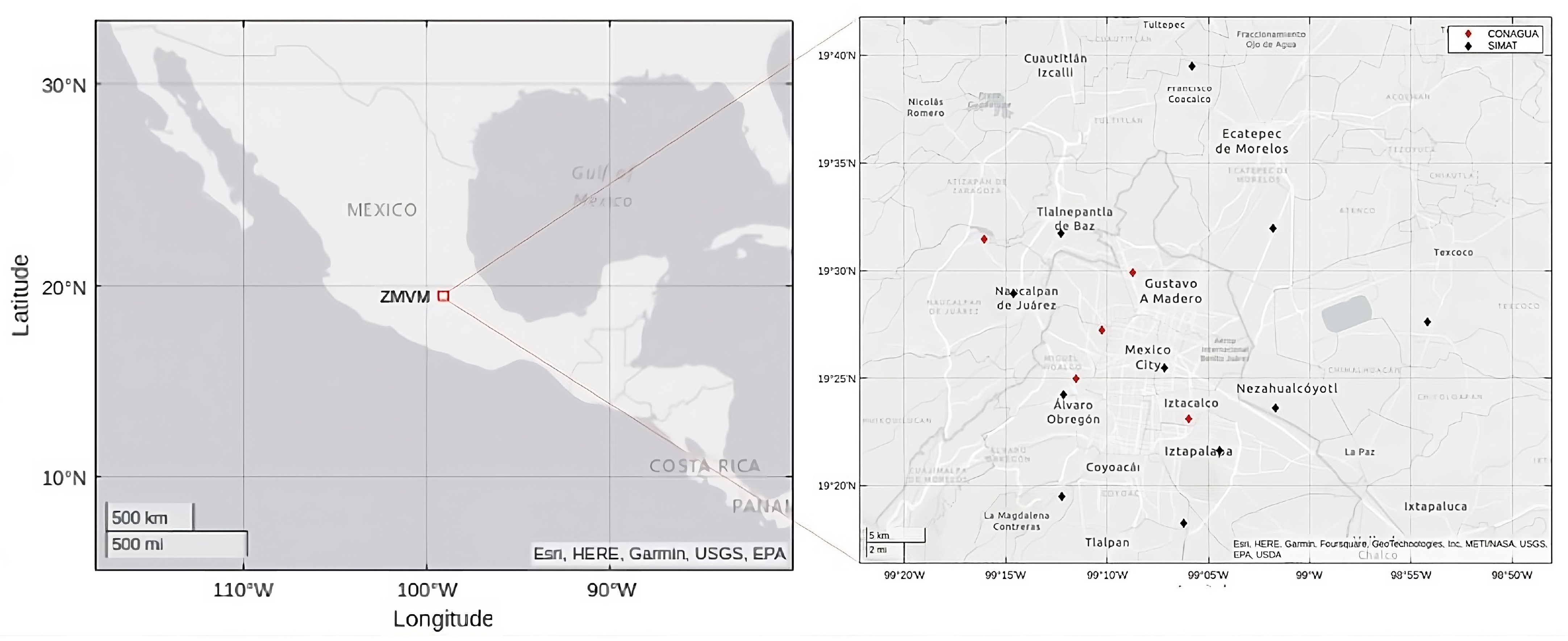
3.1. Data Set

The data used for the study were obtained from two monitoring networks in the Mexico Valley area. The data on pollutants and meteorological variables were obtained from the Automatic Atmospheric Monitoring Network (RAMA) and the Meteorological Network (REDMET) of the Atmospheric Monitoring System of Mexico City (SIMAT) of the Environmental Secretariat of the Government of Mexico City [15]. Solar radiation data were obtained from the EMA stations of the CONAGUA monitoring network [16]. The study period covers from the years 2015 to 2022. The geolocation of the measurement points is shown in Figure 1.

3.2. Feature Vector Construction

Feature vector construction is a critical step in the machine learning pipeline that has a profound impact on every subsequent step, from model training and evaluation to the interpretability of the results. It involves not just selecting the right features but also appropriately processing and engineering these features to best represent the problem space for the learning algorithm, hence the importance of understanding the variables within our research domain and their relationships in order to extract patterns from our data and enhance the precision of our predictions. Next, we will delve into the various factors and their influence on ozone concentrations.

The concentration of tropospheric ozone ($O_3$) is influenced by various atmospheric and meteorological factors, as mentioned in the research in

Table 1. Overview of research on machine learning applications for air quality forecasting models.

Research Paper	Predicted	Predictors	Models	Metrics
A Machine Learning approach to investigate the build-up of surface ozone in Mexico City (2022) [6].	$O_3$.	Temperature, Relative humidity, Wind speed and direction, $NO$, $N{O}_2$, UV-A and Planetary Boundary Layer Height.	Random Forest, Gradient Boosting, Deep Neural Network.	$R^2$, Index of Agreement (IOA).
Prediction of Air Pollutants Using Supervised Machine Learning (2021) [7].	Air quality index for $P{M}_{10}$, $P{M}_{2.5}$, $N{O}_2$, $CO$, $S{O}_2$, $N{H}_3$, $O_3$.	Country, State, City, Place, Last updated, Min, Max, Average, and Pollutants($P{M}_{10}$, $P{M}_{2.5}$, $S{O}_2$, $CO$, $N{O}_2$, $O_3$).	Decision Tree, Support Vector Machine, Logistic Regression, Random Forest, Naive Bayes, K-Nearest Neighbor.	Accuracy.
Machine Learning-Based Prediction of Air Quality (2020) [8]	Air quality index for 1 h, 8 h, and 24 h.	$P{M}_{2.5}$ and $P{M}_{10}$ moving average, $O_3$ average of the last eight hours, $CO$ concentration for the last eight hours, Air uality index based on the maximum concentration of $P{M}_{10}$, $P{M}_{2.5}$, $N{O}_2$, $S{O}_2$, $O_3$ and $CO$.	Random Forest, AdaBoost, Support Vector Regression, Artificial Neural Network.	RMSE, MAE, $R^2$.
Ground-level Ozone Prediction Using Machine Learning Techniques: A Case Study in Amman, Jordan (2020) [9]	$O_3$.	Ozone, Temperature, Humidity, Wind direction, and speed, Memorable day (weekend, holiday), Day of the year.	Multi-Layer Perceptron, Support Vector Regression, Decision Tree, XGBoost.	RMSE, MAE, $R^2$.
An ensemble-based model of $P{M}_{2.5}$ concentration across the contiguous United States with high spatiotemporal resolution (2019) [10]	$P{M}_{2.5}$.	Satellite-derived aerosol optical depth, Satellite-based measurements, Chemical transport model predictions, Land-use variables, and Meteorological variables.	Ensemble Model (Neural Network, Random Forest, Gradient Boosting).	RMSE, $R^2$.
Estimation of Air Pollution in Delhi Using Machine Learning Techniques (2018) [11]	Air pollution levels for $CO$, $N{O}_2$, $O_3$, $S{O}_2$, $P{M}_{10}$, $P{M}_{2.5}$.	Vertical wind, Wind speed and direction, Temperature, and Relative humidity.	Linear Regression, Stochastic Gradient Descent, Random Forest, Decision Tree, Support Vector Regression, Multi-layer Perceptron, Gradient Boosting Adaptive Boosting.	RMSE, MAE, $R^2$.
A Machine Learning Approach for Air Quality Prediction: Model Regularization and Optimization (2018) [12].	Next day concentration for $O_3$, $P{M}_{2.5}$, $S{O}_2$.	Air temperature, Relative humidity, Wind speed, and direction, Wind gust, Precipitation accumulation, Visibility, Dew point, Wind cardinal direction, Pressure, Weather conditions, Weekday/weekend, Concentration pollutant, and Bias term.	MTL with Linear Regression.	RMSE.
Detection and Prediction of Air Pollution Using Machine Learning Models (2018) [13].	Classification of Samples into Polluted or Non-Polluted Categories, $P{M}_{2.5}$.	Temperature, Wind speed, Dew point, Pressure, $P{M}_{2.5}$ Concentration, Classification result.	Autoregression, Logistic Regression.	MA, SDA, MAE.
AirVLC: an Application for Visualizing Wind-sensitive Interpolation of Urban Air Pollution Forecasts (2016) [14].	$NO$, $N{O}_2$, $S{O}_2$, $O_3$.	Pollution level, Meteorological conditions (Temperature, Relative humidity, Pressure, Wind speed, Rain), Calendar features (Year, Month, Day in the month, Day in the week, Hour), and Traffic intensity features.	Linear Regression, Quantile Regression, K-Nearest Neighbor, Random Forest, Decision Tree.	RMSE.

, including temperature, humidity, wind direction, and wind speed. Next, we present a general overview of how each of these factors can impact ozone concentration:

• Temperature:
  • Photochemical Reactions: Ozone formation in the troposphere is a result of photochemical reactions. Higher temperatures generally increase the rate of these reactions, leading to a faster and more efficient production of ozone.
  • Stability of the Atmosphere: On hot days, especially under high-pressure systems, the atmosphere can become more stable, trapping pollutants, including ozone and its precursors, close to the ground and increasing concentrations.
  • Volatile Organic Compound (VOC) Emissions: Higher temperatures can also lead to increased emissions of VOCs from vegetation and certain human-made sources, further promoting ozone formation.
• Humidity:
  • $OH$ Radical Production: Water vapor can contribute to the formation of hydroxyl radicals ($OH$), which play a crucial role in oxidizing VOCs and other pollutants, leading to the production of ozone. However, the exact relationship between humidity and ozone production can be complex and might vary depending on other prevailing conditions.
  • Dilution: On the other hand, extremely high humidity levels can lead to condensation and cloud formation, which may reduce solar radiation, slowing down photochemical reactions.
• Wind Direction:
  • Transport of Precursors: The direction of the wind can transport ozone precursors (like $N{O}_x$ and VOCs) from their sources to other areas. For instance, if a city has major industrial zones on its eastern side and the wind is blowing from east to west, areas downwind can experience elevated ozone levels due to the transported pollutants.
  • Clean Air Advection: Conversely, winds from rural or oceanic directions can bring cleaner air, reducing ozone concentrations.
• Wind Speed:
  • Dispersion: Faster wind speeds can help disperse pollutants, diluting their concentration. This can decrease the buildup of ozone precursors in a particular area and reduce localized ozone formation.
  • Vertical Mixing: Strong winds, especially when accompanied by turbulence, can enhance the vertical mixing of the atmosphere, distributing ozone and its precursors over a larger vertical layer. This can lead to a decrease in ground-level ozone concentrations.

It’s essential to understand that these factors often interact in multifaceted ways. For instance, a hot, calm day might be conducive to ozone buildup due to reduced dispersion and enhanced photochemical reactions. However, if that hot day is also humid with cloud cover, the reduced sunlight might counteract some of the enhanced ozone production. For this reason, it is important to depict the relationships within the process that involves interactions between various precursor pollutants, including nitrogen oxides ($N{O}_x$, which includes $NO$ and $N{O}_2$) and volatile organic compounds (VOCs), in the presence of sunlight, as shown in the research by Lelieveld and Dentener [17], or in that by Finlayson-Pitts and Pitts [18]. Next, we provide a breakdown of this phenomenon:

• Emission of Precursors: Primary pollutants like nitrogen oxides ($N{O}_x$) and volatile organic compounds (VOCs) are emitted into the atmosphere. These are typically released from automobile exhaust, industrial processes, power plants, and other combustion processes.
• Photodissociation of Nitrogen Dioxide ($N{O}_2$):

  $$N{O}_2+h\nu \to NO+O$$

  (1)
  In the presence of sunlight, $N{O}_2$ undergoes photodissociation, breaking down into nitrogen monoxide ($NO$) and a free oxygen atom (O). The symbol “$hv$” represents a photon of sunlight.
• Formation of ozone:

  $$O+O_2\to O_3$$

  (2)
  The free oxygen atom (O) rapidly reacts with molecular oxygen ($O_2$) in the atmosphere to form ozone ($O_3$).
• Reconversion:

  $$NO+O_3\to N{O}_2+O_2$$

  (3)
  Nitrogen monoxide ($NO$) can also react with the ozone ($O_3$) to form nitrogen dioxide ($N{O}_2$) and molecular oxygen ($O_2$). This essentially reduces the concentration of ozone.
• VOCs Role in the Cycle: VOCs, in the presence of $N{O}_x$ and sunlight, can generate more reactive intermediates, which will react with $NO$ to form $N{O}_2$. This reaction “removes” $NO$ from the environment, allowing more ozone to form without it being quickly converted back to oxygen. In other words, the VOCs help “tie up” $NO$, preventing it from immediately destroying the ozone that’s been formed.

Finally, it is important to show how the ozone concentration could be influenced by temporal factors such as the month, day of week, and hour, or by geospatial factors as longitude, latitude and altitude; you can see a brief explanation of how each of these variables might impact ozone concentration:

• Month:
  • Sunlight Intensity and Duration: Ozone formation is a photochemical process that requires sunlight. Therefore, months with longer daylight hours and more intense sunlight, typically the spring and summer months, tend to have higher ozone concentrations.
  • Temperature: Months with warmer temperatures, typically summer months, can lead to higher ozone concentrations.
  • Vegetation Growth and Emissions: Certain months, especially spring and early summer, might see increased biogenic emissions of volatile organic compounds (VOCs) from vegetation, which can contribute to ozone formation.
• Day of week:
  • Emissions Variability: Weekdays often have higher vehicular traffic and industrial activities compared to weekends. This can lead to higher emissions of ozone precursors like $N{O}_x$ on weekdays.
  • Weekend Effect: Despite reduced precursor emissions on weekends, some urban areas observe higher ozone levels during weekends, a phenomenon known as the “weekend effect”. This can be due to the disproportionate reduction in $NO$ emissions compared to VOCs on weekends, altering the chemical balance and facilitating ozone production.
• Hour:
  • Daily Cycle: Shown in the ozone concentration pattern, there are usually lower levels in the early morning because the sun has not risen or is low in the sky, reducing the intensity of UV radiation needed for ozone formation; ozone peaks during the afternoon when sunlight is most intense and temperatures are highest; in the evening, the rate of ozone production decreases, but the loss processes are slower. UV radiation needed for ozone formation changes throughout the day, affecting the intensity of UV radiation reaching the surface.
  • Emissions Patterns: Human activities, such as traffic and industrial operations, have specific hourly patterns.
  • Mixing Layer Depth: The depth of the atmospheric mixing layer changes throughout the day, affecting the dispersion of pollutants.
• Latitude:
  • Sunlight Intensity: Near the equator (low latitudes), the sun’s rays are more direct, leading to more intense UV radiation, which can enhance photochemical reactions and thus ozone formation.
  • Distribution of Emission Sources: Industrialized regions and urban centers, significant sources of ozone precursors like $N{O}_x$ and VOCs, may be concentrated at specific latitudes.
  • Stratospheric Intrusions: At high latitudes, stratospheric intrusions can introduce ozone-rich air from the stratosphere to the troposphere.
• Longitude:
  • Time of Day: Due to the Earth’s rotation, the position of the sun changes with longitude, affecting the daily cycle of photochemical reactions.
  • Distribution of Emission Sources: Significant emission sources might be concentrated at specific longitudes.
  • Meteorological Patterns: Weather systems vary longitudinally, especially in regions influenced by oceanic or continental effects.
• Altitude:
  • Decreased Pressure: As altitude increases, atmospheric pressure decreases, potentially affecting ozone formation.
  • Temperature Profile: The temperature can either increase or decrease with altitude, affecting ozone concentrations.
  • Vertical Distribution of $O_3$: Ozone concentrations generally increase with altitude in the troposphere and are high in the stratosphere.
  • Transport of Ozone Precursors: Elevated regions might be exposed to ozone precursors transported from lower altitudes.

With the goal of predicting ozone concentrations in the study area with a 24-h lead time, considering the existing relationships between these variables and the influence they have on said concentrations, the feature vector was formed, as shown in

Table 2. Feature vector.

Temporal and Geospatial Variables
longitude	latitude		altitude	month	weekday		hour
24 h prior meteorological and pollutant variables
$O_3$	$NO$	$N{O}_2$	$N{O}_x$	Relative humidity (rh)	Temperature (tmp)	Wind direction (wdr)	Wind speed (wsp)
Solar radiation from EMAs stations 24 h prior
ECOGUARDAS	TEZONTLE		MOLINODELREY	ENCBI	ENCBII		PRESAMADIM
Meteorological variables			Pollutant variables		EMAs Stations
Mean 00to03			Mean 00to03		Mean 00to03
Mean 04to07			Mean 04to07		Mean 04to07
Mean 08to11			Mean 08to11		Mean 08to11
Mean 12to15			Mean 12to15		Mean 12to15
Mean 16to19			Mean 16to19		Mean 16to19
Mean 20to23			Mean 20to23		Mean 20to23
previous day’s maximum			previous day’s maximum		previous day’s maximum
previous day’s minimum			previous day’s minimum		previous day’s minimum

The feature vector consists of 132 variables.

.

3.3. Hyperparameter Optimization

The optimization of hyperparameters in machine learning models is a process of critical importance, significantly impacting model performance and accuracy. This procedure involves fine-tuning the hyperparameters, which govern the learning algorithm’s behavior and its capability to accurately interpret and learn from underlying data patterns. Optimal hyperparameter settings enhance the model’s performance and improve the results obtained. One of the key roles of hyperparameter optimization is to mitigate the risks of overfitting and underfitting, striking a balance where the model is sufficiently complex to elucidate essential data patterns without being excessively tailored to the training data. This balance is crucial in ensuring the model’s ability to generalize effectively from training data to new, unseen data. There are different approaches to address this issue, as mentioned by Feurer and Hutter [19]. In this research, we decided to use GridSearchCV, which has some significant advantages in its implementation but also presents some disadvantages that we need to address. The operational scheme of GridsearchCV is based on the wrapper method proposed by Kohavi and Jonh [20] and is shown in Figure 2.

GridSearchCV is a systematic approach employed in the field of machine learning for the optimization of model hyperparameters. This method is instrumental in enhancing the performance of a machine learning model by exhaustively searching through a predefined space of hyperparameter values. The fundamental premise of Grid Search is to evaluate and compare the model’s performance across different combinations of hyperparameters, thereby identifying the most effective set of parameters. This process of GridSearch involves the following key steps:

• Definition of Hyperparameter Space: The first step involves delineating the range or set of values for each hyperparameter under consideration. This set forms a grid of hyperparameter combinations, where each node represents a unique combination. The generation of this grid of options and evaluating all solutions is a task that demands too many resources and is impossible to carry out because many hyperparameters take continuous values. Therefore, it is chosen to define recommended or well-known ranges of values for these hyperparameters, creating a finite space of combinations.
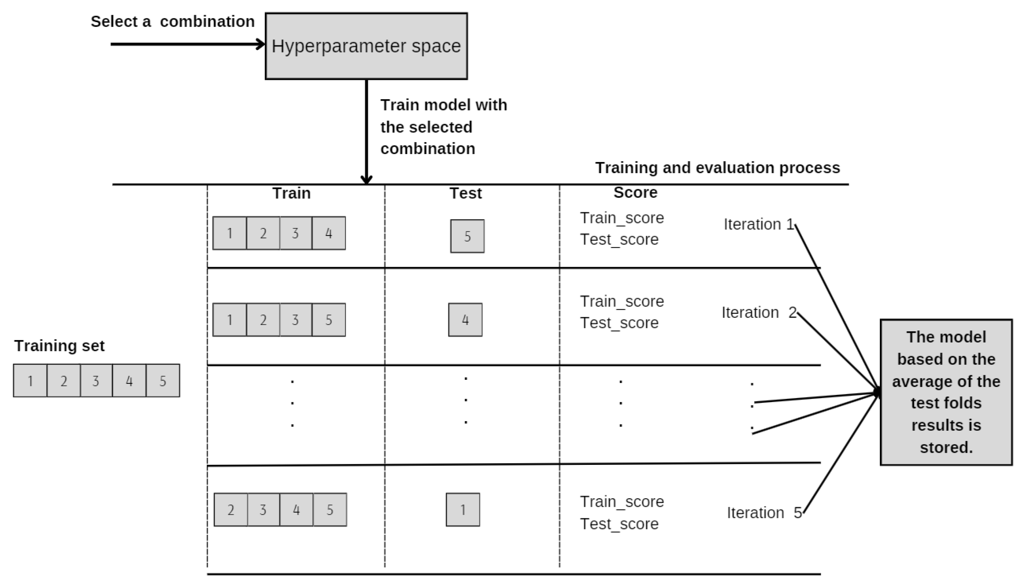
• Cross-Validation Mechanism: GridSearch is typically coupled with cross-validation to assess the performance of the model for each hyperparameter combination. Cross-validation involves dividing the training dataset into multiple smaller sets or folds. The model is trained on all but one fold (the training set) and validated on the remaining fold (the test set). This process is repeated so that each fold serves as the validation set once, ensuring comprehensive evaluation.
  The utilization of cross-validation helps to improve the model’s performance by reducing variance through averaging performance estimates from multiple iterations of training and testing on different data subsets. It presents a better generalization by evaluating the model on multiple subsets of the data, aiding in assessing its generalization capabilities. This is especially important for detecting overfitting, as the model’s performance is evaluated on various data partitions, resulting in a more robust estimate of its accuracy on unseen data, as is mentioned in the study guided by Kohavi [21].
• Selection of Optimal Hyperparameters: Post evaluation, the combination of hyperparameters that produces the best performance is selected based on the minimal average error of the test folds.

As mentioned before, GridSearchCV presents the advantages of increasing the model’s precision and improving the generalization and potentially reduced bias in the estimation of model performance. Another advantage is that it facilitates the comparison between various model families because, although each model has its own sets of hyperparameters, the evaluation is performed based on the same metric to measure the error. On the other hand, its main disadvantage is the computational complexity that can arise for very large datasets or complex models.

The optimization process in this research was conducted utilizing the GridSearchCV tool from the Scikit-learn library [22]. The models subjected to testing included RandomForest [23], GradientBoosting [24], and Support Vector Regression (SVR) [25]. In the case of SVR, a pipeline was established to assess the impact of data scaling, involving MinMax normalization and Z-score standardization, alongside hyperparameter tuning. The comprehensive list of hyperparameters is presented in

Table 3. Evaluated models.

Model	Hyperparameters
RandomForest	Max depth: 40–50
	Max features: 10–25
SVR (kernel RBF)	Scaling: [StandardScaler, MinMaxScaler]
	Gamma: [0.001, 0.01, 0.1, 1, 10, 100]
	C: [0.001, 0.01, 0.1, 1, 10, 100]
SVR (kernel poly)	Scaling: [StandardScaler, MinMaxScaler]
	Degree: [2, 3, 4, 5, 6, 7, 8, 9]
	C: [0.001, 0.01, 0.1, 1, 10, 100]
GradientBoosting	n estimators: [1, 2, 5, 10, 20, 50, 100, 200, 300]
	Max depth: [5, 6, 7, 8, 9, 10, 11, 12, 13, 14, 15, 16, 17, 18, 19]
	Learning rate: [0.001, 0.01, 0.1, 0.2, 0.3, 0.4, 0.5, 0.6, 0.7, 0.8, 0.9]

.

GridSearchCV is a process that can be time-consuming because it must test every combination of hyperparameters on the training sets. For this reason, Cochran’s formula [26] was used for sample size selection for quantitative variables when the population size is known to train the models with a smaller sample size and reduce execution time. The formula used is shown in Equation (4).

$$n=\frac{N{Z}^2{\sigma }^2}{(N-1)E^2+Z^2{\sigma }^2}$$

(4)

where:

n	= sample size.
N	= population size.
Z	= critical Z value; for a confidence level of $99\%$, z equals 2.58.
${\sigma }^2$	= population variance.
E	= absolute precision level; $1\%$ of the population’s standard deviation.

The dataset, containing data from 2015 to 2022, comprises 577,031 records. The sample size selection formula determined that a sample size of 59,680 records would provide a $99\%$ confidence level, representing $10.34\%$ of the total records. For the validation sample, $10\%$ of the complete dataset was chosen, resulting in 57,704 records. It is important to note that the training and validation sets are entirely exclusive.

3.4. Model Evaluation

As shown in the hourly profile in Figure 3, ozone concentration exhibits a clear trend with the time of day, and there is significant variation compared to the study period’s mean. To effectively measure the performance of the evaluated models, their performance will be evaluated using two approaches. The first approach will involve comparing the MAE of the models with the MAE calculated for predictions based on Mean and Median strategies throughout the entire period from 2015 to 2022. The second approach will compare the MAE based on Mean and Median strategies, grouping by hour to evaluate which of the models performs better throughout the hours of the day. The reference MAE values are presented in

Table 4. Baseline Mean Absolute Error.

Timeframe	MAE from Mean	MAE from Median	Timeframe	MAE from Mean	MAE from Median
2015–2022	21.53	20.77
00:00	9.03	8.95	12:00	15.83	15.82
01:00	8.85	8.77	13:00	17.82	17.81
02:00	8.50	8.39	14:00	19.10	19.09
03:00	8.01	7.84	15:00	19.38	19.34
04:00	6.87	6.54	16:00	18.69	18.63
05:00	5.08	4.45	17:00	16.53	16.43
06:00	3.42	2.85	18:00	14.01	13.91
07:00	4.01	3.67	19:00	12.54	12.43
08:00	6.66	6.52	20:00	11.24	11.13
09:00	9.38	9.31	21:00	10.37	10.26
10:00	12.03	11.94	22:00	9.70	9.60
11:00	13.92	13.88	23:00	9.33	9.26

The MAE was calculated using predictions based on both the mean and median strategies applied to the complete dataset.

.

3.5. Setup for the Experiment

The programs were executed on a Beowulf cluster with Torque 3.0.3, using four computing nodes running Ubuntu 20.04.4. Each node was equipped with 2 Intel(R) Xeon(R) CPU E5-2640 v4 processors @ 2.40 GHz, featuring 20 processing cores and 128 GB of RAM. The software versions used were Anaconda 22.9.0, Python 3.9.12, and Scikit-learn 1.0.2.

4. Results

4.1. GridSearch

The results presented in

Table 5. Gridsearch results.

Model	Hyperparameters	Test Score	Train Score	Gap
RandomForest Execution time: 2600	max depth = 45, max  features = 25.	7.825020	2.923992	4.901028
StandardScaler → SVR (RBF) Execution time: 29,672	C = 100, gamma = 0.01.	7.845238	3.350762	4.494476
	C = 10, gamma = 0.001.	8.757496	8.652644	0.104852
StandardScaler → SVR (poly) Execution time: 104,571	C = 100, degree = 3.	9.062664	5.348223	3.714441
	C = 10, degree = 2.	11.562271	10.979601	0.582670
MinMaxScaler → SVR (RBF) Execution time: 22,465	C = 100, gamma = 0.1.	7.785040	6.806308	0.978732
	C = 100, gamma = 0.01.	8.700342	8.617988	0.082355
MinMaxScaler → SVR (poly) Execution time: 1,705,128	C = 100, degree = 3.	7.925763	6.892926	1.032837
	C = 10, degree = 4.	8.060671	7.198237	0.862434
GradientBoosting Execution time: 42,584	learning rate = 0.1, max depth = 10, max features = 12, n estimators = 300.	7.144314	1.735895	5.408419
	learning rate = 0.1, max depth = 9, max features = 11, n estimators = 300.	7.187491	2.818148	4.369343

The grid search was executed using n_jobs = 20 option; the execution time unit is in seconds.

were selected using the following criteria: the top five results were chosen for each of the models, from which the one with the lowest MAE in the test results and the one with the slightest difference between the training and test score (gap) were selected. In the case of the RandomForest model, the result with the lowest MAE in the test set also had the slightest difference between the training and test sets.

4.2. Optimal Model Selection

Each model listed in Table 5 underwent a comprehensive evaluation utilizing a dataset comprising 57,704 records. The derived results, systematically arranged in descending order based on their respective evaluation scores, are detailed in

Table 6. Model results.

Model	Fit Time	Evaluation Score 1
GradientBoosting[0] 2	522	7.015008
GradientBoosting[1]	423	7.126916
StandardScaler → SVR (RBF)[0]	54,058	7.689650
RandomForest	392	7.808124
MinMaxScaler → SVR (poly)[0]	8172	7.901960
MinMaxScaler → SVR (poly)[1]	3250	8.037673
MinMaxScaler → SVR (RBF)[0]	1968	8.717526
StandardScaler → SVR (RBF)[1]	4191	8.758239
StandardScaler → SVR (poly)[0]	73,851	9.468176
MinMaxScaler → SVR (RBF)[1]	1959	10.733147
StandardScaler → SVR (poly)[1]	4242	11.405547

¹ The results are organized in descending order based on their evaluation scores. ² The number inside the brackets represents the position within the hyperparameters column in Table 5 for each of the models.

. Notably, every model demonstrated superior performance compared to the median of the Mean Absolute Error (MAE) observed during 2015–2022. However, selecting the optimal model requires an in-depth assessment beyond mere evaluation scores. This includes a detailed analysis of the models’ hourly MAE fluctuations, as depicted in Figure 4. Additionally, a critical review of each model’s computational efficiency, particularly their execution times during both the GridSearch process and subsequent training phases, is essential. This aspect of model performance is thoroughly explicated in Figure 5.

5. Discussion

This section is bifurcated into two distinct segments for a comprehensive analysis. The first segment delves into a generalized discussion centered around the performance outcomes discerned from the hyperparameter optimization processes and an evaluation of the models selected thereafter. The second segment, on the other hand, is dedicated to an in-depth analysis of the best-performing model identified through these processes.

5.1. General Discussion

In the GridSearch results, RandomForest showed the shortest execution time and acceptable training times with results in the Training and Testing. However, it is one of the models with the greatest difference between the Training and Test sets, indicating a slight overfitting. The SVR models that use the RBF kernel outperformed their counterparts with the polynomial kernel in terms of execution times, and they did not show significant differences in their Test scores. In general, the SVR-based models had the lowest level of overfitting, as they exhibited the smallest differences in the Training–Test gap. However, it is essential to consider the computational complexity of this model because it will consume much time when the number of records exceeds 10,000, especially when using Sklearn’s SVR implementation based on libsvm. This implementation has complexities greater than quadratic $n^2$, as mentioned by Abdiansah and Wardoyo [27]. GradientBoosting achieved the best results for Train and Test scores with quite acceptable times, although it did show a higher level of overfitting due to differences in the Train–Test gap.

Concerning the evaluation results, as can be seen in Figure 4, the top five selected models show acceptable performance in terms of the MAE calculated by the time of day range, exhibiting a similar behavior. It is worth noting that the models reflect the ozone hourly profile quite well, as they capture the periods with the highest MAE during the hours when ozone concentration varies the most, from 12:00 to 18:00, as shown in Figure 3. GradientBoosting[0] exhibited lower MAE from 00:00 to 11:00, 13:00–14:00, and 17:00–22:00, while GradientBoosting[1] performed better at 12:00, 15:00–16:00, and 23:00. Therefore, the first model was selected as the one with the best performance.

An additional critical factor to consider in model selection is the execution time associated with different models, especially when dealing with a substantial volume of records. This aspect becomes increasingly significant, as large datasets can entail considerable processing durations. Consequently, the ability to conduct preliminary phases of hyperparameter optimization and model evaluation efficiently, utilizing a smaller yet adequately representative subset of the data, is imperative for effectively identifying and selecting the most suitable model.

5.2. Analysis of the Optimal Performing Model

Figure 6 presents an analysis of the performance exhibited by the GradientBoosting[0] model, designated as GB_99, which was trained on a subset comprising 59,680 records. This subset accounts for $10.34\%$ of the training dataset and is statistically significant, offering a $99\%$ confidence level, as delineated in Equation (4). In contrast, the model labeled GB_full refers to the GradientBoosting[0] variant trained on the entirety of the training dataset, encompassing 519,327 records. Additionally, the graph includes MEAN and MEDIAN, which indicate the MAE values when predictions are based on these respective statistical measures. This comparison offers insight into the efficacy and scalability of the GradientBoosting[0] model under varying training data volumes and their performance against the MEAN and MEDIAN prediction approaches.

Table 7. Optimal Model’s Hourly MAE Performance.

Timeframe	GB_99	GB_full	Timeframe	GB_99	GB_full
00:00	6.772	5.754	12:00	9.444	6.893
01:00	6.172	5.223	13:00	10.905	7.919
02:00	5.709	4.718	14:00	11.932	8.639
03:00	5.595	4.645	15:00	12.345	8.546
04:00	4.9	3.941	16:00	11.413	8.22
05:00	3.76	2.958	17:00	9.582	7.125
06:00	3.054	2.39	18:00	7.443	5.932
07:00	3.088	2.369	19:00	6.824	5.493
08:00	4.239	3.441	20:00	6.6	5.428
09:00	5.44	4.377	21:00	6.521	5.217
10:00	6.628	5.218	22:00	5.924	4.885
11:00	7.789	6.05	23:00	5.565	4.567

In total, 57,704 records were used to calculate the MAE for the GB_99 model, while in the case of GB_full, 519,327 records were used.

compares the hourly MAE performance for the GradientBoosting[0] model. Here are some observations and opinions on these data:

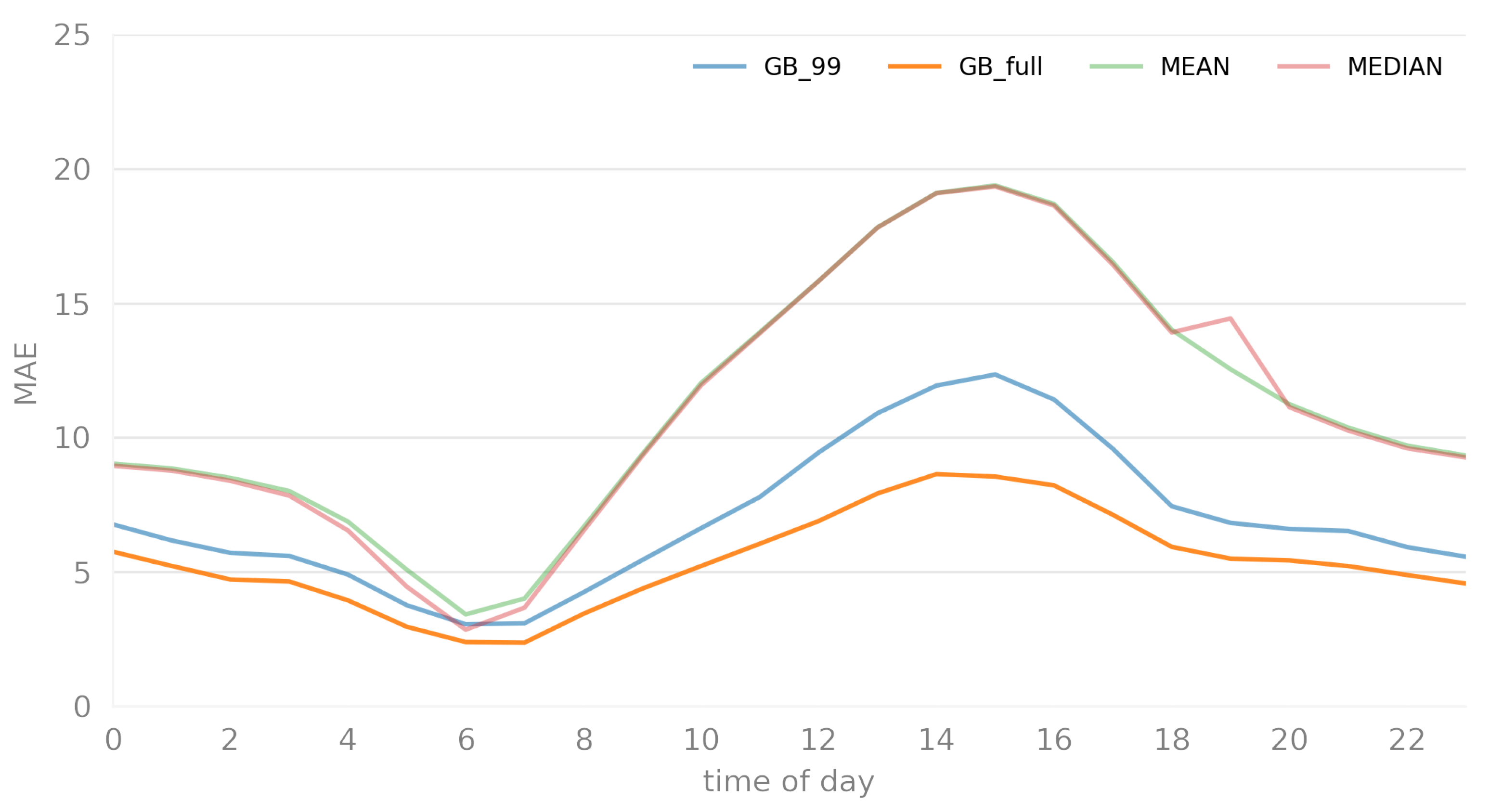
• Data Size Impact: The GB_full model, trained on a significantly larger dataset (519,327 records) compared to GB_99 (57,704 records), consistently shows lower MAE across all timeframes. This indicates the potential benefits of training on more extensive data, likely capturing more nuances and patterns, leading to better predictive performance.
• Performance Consistency: Both models exhibit a similar pattern in MAE fluctuations over the 24 h, suggesting that the underlying data characteristics influencing error rates are similar for both datasets. However, the magnitude of the error is consistently lower in the GB_full model, reinforcing the value of a more extensive training set.
• Timeframe Sensitivity: There are periods (like early morning hours) where the MAE is relatively lower for both models and periods (like afternoon to early evening) where MAE peaks. This pattern could indicate varying model performance based on time-specific factors, suggesting that certain hours have characteristics that are either more predictable or more challenging for the model.

The comparison between the “Optimal Model’s Hourly MAE Performance” (Table 7) and the “Baseline Mean Absolute Error” (Table 4) is quite revealing in terms of understanding the effectiveness of the Gradient Boosting (GB) models relative to basic baseline methods. Here are some observations and opinions on these data:

• Significant Improvement Over Baseline: Both Gradient Boosting models (GB_99 and GB_full) consistently outperform the baseline models across almost all timeframes. The MAEs for the baseline methods are significantly higher than those for the Gradient Boosting models, indicating the superior predictive capability of the latter.
• Effectiveness of Machine Learning Models: The considerable reduction in MAE when using the Gradient Boosting models compared to the baseline methods illustrates the value of machine learning in capturing complex patterns and relationships in the data that simple statistical measures cannot.

6. Conclusions

Based on the results obtained in the present research, the following conclusions have been reached:

• Machine learning models are a significant alternative for ozone concentration forecasting. However, it is paramount to identify the variables influencing the phenomenon in constructing the feature vector. This enables the models to discern patterns and relationships among the variables correctly.
• Computational complexity can significantly impact the best model selection, as the computational resources required for hyperparameter optimization can be time-consuming and may not be feasible.
• A substantial volume of historical records to train models can enhance their precision. However, certain models do not efficiently handle large datasets, leading to disproportionately increased evaluation times. Therefore, employing a technique that allows for selecting a sufficiently representative sample to achieve results with an acceptable level of reliability without adversely affecting the outcomes of the models is of paramount importance. This approach ensures both the effectiveness and efficiency of the model training and evaluation process.
• Establishing a baseline is a critical step in model evaluation. It helps set realistic expectations and understand the value added by complex models.
• The GB models’ lower MAE scores, especially compared to the relatively high baseline MAEs, suggest that these models have successfully captured significant underlying trends and patterns in the hourly ozone concentration profile.
• Elevated errors observed during specific time intervals warrant further investigation as potential focal points for future enhancements in model performance. Delving into the underlying reasons for these heightened error rates during particular hours and exploring what additional data or modifications in feature engineering might mitigate these discrepancies could yield significant advancements in model accuracy and reliability.
• Tree-based models like Random Forests or Gradient Boosting demonstrated better generalization to unseen data, but they tend to be more prone to overfitting than SVR models. This might necessitate more frequent retraining of tree-based models compared to SVR. However, given their shorter training times, they still present a better option in terms of model maintainability.

References

- Molina, L.T.; Madronich, S.; Gaffney, J.S.; Apel, E.; de Foy, B.; Fast, J.; Ferrare, R.; Herndon, S.; Jimenez, J.L.; Lamb, B.; et al. An overview of the MILAGRO 2006 Campaign: Mexico City emissions and their transport and transformation. Atmos. Chem. Phys. 2010, 10, 8697–8760. [Google Scholar] [CrossRef]
- Rojas-Martinez, R.; Perez-Padilla, R.; Olaiz-Fernandez, G.; Mendoza-Alvarado, L.; Moreno-Macias, H.; Fortoul, T.; McDonnell, W.; Loomis, D.; Romieu, I. Lung Function Growth in Children with Long-Term Exposure to Air Pollutants in Mexico City. Am. J. Respir. Crit. Care Med. 2007, 176, 377–384. [Google Scholar] [CrossRef] [PubMed]
- Baldasano, J.; Valera, E.; Jimenez, P. Air quality data from large cities. Sci. Total Environ. 2003, 307, 141–165. [Google Scholar] [CrossRef] [PubMed]
- Karthik L, B.; Sujith, B.; Rizwan A, S.; Sehgal, M. Characteristics of the Ozone Pollution and its Health Effects in India. Int. J. Med. Public Health 2017, 7, 56–60. [Google Scholar] [CrossRef]
- Niu, Y.; Zhou, Y.; Chen, R.; Yin, P.; Meng, X.; Wang, W.; Liu, C.; Ji, J.S.; Qiu, Y.; Kan, H.; et al. Long-term exposure to ozone and cardiovascular mortality in China: A nationwide cohort study. Lancet Planet. Health 2022, 6, e496–e503. [Google Scholar] [CrossRef] [PubMed]
- Ahmad, M.; Rappenglück, B.; Osibanjo, O.; Retama, A. A machine learning approach to investigate the build-up of surface ozone in Mexico-City. J. Clean. Prod. 2022, 379, 134638. [Google Scholar] [CrossRef]
- Yarragunta, S.; Nabi, M.A.; Jeyanthi, P.; Revathy, S. Prediction of Air Pollutants Using Supervised Machine Learning. In Proceedings of the 2021 5th International Conference on Intelligent Computing and Control Systems (ICICCS), Madurai, India, 6–8 May 2021; pp. 1633–1640. Available online: https://ieeexplore.ieee.org/document/9432078 (accessed on 30 November 2023).
- Liang, Y.C.; Maimury, Y.; Chen, A.H.L.; Juarez, J.R.C. Machine Learning-Based Prediction of Air Quality. Appl. Sci. 2020, 10, 9151. [Google Scholar] [CrossRef]
- Aljanabi, M.; Shkoukani, M.; Hijjawi, M. Ground-level Ozone Prediction Using Machine Learning Techniques: A Case Study in Amman, Jordan. Int. J. Autom. Comput. 2020, 17, 667–677. [Google Scholar] [CrossRef]
- Di, Q.; Amini, H.; Shi, L.; Kloog, I.; Silvern, R.; Kelly, J.; Sabath, M.B.; Choirat, C.; Koutrakis, P.; Lyapustin, A.; et al. An ensemble-based model of PM2.5 concentration across the contiguous United States with high spatiotemporal resolution. Environ. Int. 2019, 130, 104909. [Google Scholar] [CrossRef]
- Srivastava, C.; Singh, S.; Singh, A.P. Estimation of Air Pollution in Delhi Using Machine Learning Techniques. In Proceedings of the 2018 International Conference on Computing, Power and Communication Technologies (GUCON), Greater Noida, India, 28–29 September 2018; pp. 304–309. [Google Scholar] [CrossRef]
- Zhu, D.; Cai, C.; Yang, T.; Zhou, X. A Machine Learning Approach for Air Quality Prediction: Model Regularization and Optimization. Big Data Cogn. Comput. 2018, 2, 5. [Google Scholar] [CrossRef]
- Aditya, C.R.; Deshmukh, C.R.; Nayana, D.K.; Vidyavastu, P.G. Detection and Prediction of Air Pollution using Machine Learning Models. Int. J. Eng. Trends Technol. 2018, 59, 204–207. [Google Scholar] [CrossRef]
- Contreras-Ochando, L.; Ferri, C. airVLC: An Application for Visualizing Wind-Sensitive Interpolation of Urban Air Pollution Forecasts. In Proceedings of the 2016 IEEE 16th International Conference on Data Mining Workshops (ICDMW), Barcelona, Spain, 12–15 December 2016; pp. 1296–1299. Available online: https://ieeexplore.ieee.org/document/7836819 (accessed on 30 November 2023).
- CDMX, G. Dirección de Monitoreo Atmosférico. 2003. Available online: http://www.aire.cdmx.gob.mx/aire/default.php (accessed on 18 January 2023).
- México, G. Estaciones Meteorológicas Automáticas (EMAS). 2008. Available online: https://smn.conagua.gob.mx/es/observando-el-tiempo/estaciones-meteorologicas-automaticas-ema-s (accessed on 23 March 2023).
- Lelieveld, J.; Dentener, F.J. What controls tropospheric ozone? J. Geophys. Res. Atmos. 2000, 105, 3531–3551. [Google Scholar] [CrossRef]
- Finlayson-Pitts, B.; Pitts, J. Atmospheric Chemistry of Tropospheric Ozone Formation: Scientific and Regulatory Implications. Air Waste 1993, 43, 1091–1100. [Google Scholar] [CrossRef]
- Feurer, M.; Hutter, F. Hyperparameter Optimization. In Automated Machine Learning; Hutter, F., Kotthoff, L., Vanschoren, J., Eds.; Series Title: The Springer Series on Challenges in Machine Learning; Springer: Cham, Switzerland; pp. 3–33. Available online: https://link.springer.com/chapter/10.1007/978-3-030-05318-5_12019 (accessed on 30 November 2023).
- Kohavi, R.; John, G.H. Automatic Parameter Selection by Minimizing Estimated Error. In Machine Learning Proceedings 1995; Elsevier: Amsterdam, The Netherlands, 1995; pp. 304–312. Available online: https://www.sciencedirect.com/science/article/abs/pii/B9781558603776500451?via%3Dihub (accessed on 30 November 2023).
- Kohavi, R. A Study of Cross-Validation and Bootstrap for Accuracy Estimation and Model Selection. In Proceedings of the 14th International Joint Conference on Artificial Intelligence-Volume 2, Montreal, QC, Canada, 20–25 August 1995; IJCAI’95. pp. 1137–1143. [Google Scholar]
- Pedregosa, F.; Varoquaux, G.; Gramfort, A.; Michel, V.; Thirion, B.; Grisel, O.; Blondel, M.; Prettenhofer, P.; Weiss, R.; Dubourg, V.; et al. Scikit-learn: Machine Learning in Python. J. Mach. Learn. Res. 2011, 12, 2825–2830. [Google Scholar]
- Liu, Y.; Wang, Y.; Zhang, J. New Machine Learning Algorithm: Random Forest. In Information Computing and Applications; Series Title: Lecture Notes in Computer Science; Hutchison, D., Kanade, T., Kittler, J., Kleinberg, J.M., Mattern, F., Mitchell, J.C., Naor, M., Nierstrasz, O., Pandu Rangan, C., Steffen, B., et al., Eds.; Springer: Berlin/Heidelberg, Germany, 2012; Volume 7473, pp. 246–252. [Google Scholar] [CrossRef]
- Friedman, J.H. Greedy Function Approximation: A Gradient Boosting Machine. Ann. Stat. 2001, 29, 1189–1232. [Google Scholar] [CrossRef]
- Smola, A.J.; Schölkopf, B. A tutorial on support vector regression. Stat. Comput. 2004, 14, 199–222. [Google Scholar] [CrossRef]
- Cochran, W.G. Sampling Techniques, 3rd ed.; John Wiley: Hoboken, NJ, USA, 1977. [Google Scholar]
- Abdiansah, A.; Wardoyo, R. Time Complexity Analysis of Support Vector Machines (SVM) in LibSVM. Int. J. Comput. Appl. 2015, 128, 28–34. [Google Scholar] [CrossRef]