A Novel Hybrid Spatiotemporal Missing Value Imputation Approach for Rainfall Data: An Application to the Ratnapura Area, Sri Lanka

Abstract

Meteorological time series, such as rainfall data, show spatiotemporal characteristics and are often faced with the problem of containing missing values. Discarding missing values or modeling data with missing values causes negative impacts on the accuracy of the final predictions. Hence, accurately estimating missing values by considering the spatiotemporal variations in data has become a crucial step in eco-hydrological modeling. The multi-layer perceptron (MLP) is a promising tool for modeling temporal variation, while spatial kriging (SK) is a promising tool for capturing spatial variations. Therefore, in this study, we propose a novel hybrid approach combining the multi-layer perceptron method and spatial kriging to impute missing values in rainfall data. The proposed approach was tested using spatiotemporal data collected from a set of nearby rainfall gauging stations in the Ratnapura area, Sri Lanka. Missing values are present in collected rainfall data consecutively for a considerably longer period. This pattern has scattered among stations discontinuously over five years. The proposed hybrid model captures the temporal variability and spatial variability of the rainfall data through MLP and SK, respectively. It integrates predictions obtained through both MLP and SK with a novel optimal weight allocation method. The performance of the model was compared with individual approaches, MLP, SK, and spatiotemporal kriging. The results indicate that the novel hybrid approach outperforms spatiotemporal kriging and the other two pure approaches.

1. Introduction

1.1. Background

Rainfall is a natural phenomenon that shows spatiotemporally varying behavior. These characteristics with chaotic dynamic patterns make it difficult to predict its future behavior. Moreover, a common shortcoming of rainfall data is the inherent inclusion of missing values. This is because the data are collected from different gauging stations located in a widespread geographical area. The malfunctioning of equipment, relocation of gauging stations, network interruptions, natural hazards, and emergencies like pandemics may disturb the continuous measurement of this natural phenomenon [1].

Ignoring the stations with missing data leads to an information loss due to the strong spatial correlation between meteorological stations. On the other hand, modeling rainfall data with missing values negatively impacts the accuracy of rainfall models due to the discontinuity of the time sequence [2]. Hence, identification of a suitable mechanism to address this issue is a crucial step in an effective rainfall forecasting.

When the missing values occur at random, modeling them to estimate their values is not required. However, if the missing values are not random, then the missingness cannot be ignored and must be modeled and predicted [3]. This is known as missing value imputation and it is carried out as a data preprocessing step. Much research has been conducted using different types of missing value imputation methods. However, studies on imputing the missing values for spatiotemporal data (including meteorological records) are rare [4,5,6,7]. This study presents a novel and more efficient spatiotemporal methodology to impute missing values in rainfall data for a few rain gauging stations. The proposed methodology was tested using rainfall data collected from six neighbouring rain gauging stations (which are considered reference stations) of Ratnapura, which was identified as the target rain gauging station in our main study of rainfall forecasting. The reason for our choice is that Ratnapura is a flood-prone area in Sri Lanka due to its frequent exposure to heavy rainfall throughout the year [8,9]. In 2003, flash flood events in Ratnapura accounted for financial damage of LKR 50.6 million [9].

1.2. Related Work

Much past research has accompanied traditional statistical and/or machine learning techniques in missing value imputation of meteorological data. Some studies only captured the spatial variations (e.g., [10,11,12,13]) using spatial interpolation methods such as the inverse distance method (ID), normal ratio method (NR), geographical co-ordinates method (GC), and spatial kriging, also known as Gaussian process regression, while others only focused on their variation over time (e.g., [14,15,16]). The most common temporal method used is the autoregressive integrated moving average (ARIMA) models.

Some studies (e.g., [17]) pointed out that the predictions obtained from spatiotemporal methods are more accurate than those of purely spatial predictions. This is mainly because spatiotemporal interpolation can be applied to geo-referencing positions over a space–time grid. Some researchers have used the traditional spatial kriging model after some modifications to model the spatiotemporal behavior of the data [4,5].

There have been several spatiotemporal kriging-based studies conducted with weather variables. The study in [18] developed a spatiotemporal kriging model to predict wind speed and compared the results with the autoregressive moving average (ARMA) and Monte Carlo methods. Spatiotemporal kriging modeling gave a better fit for the data.

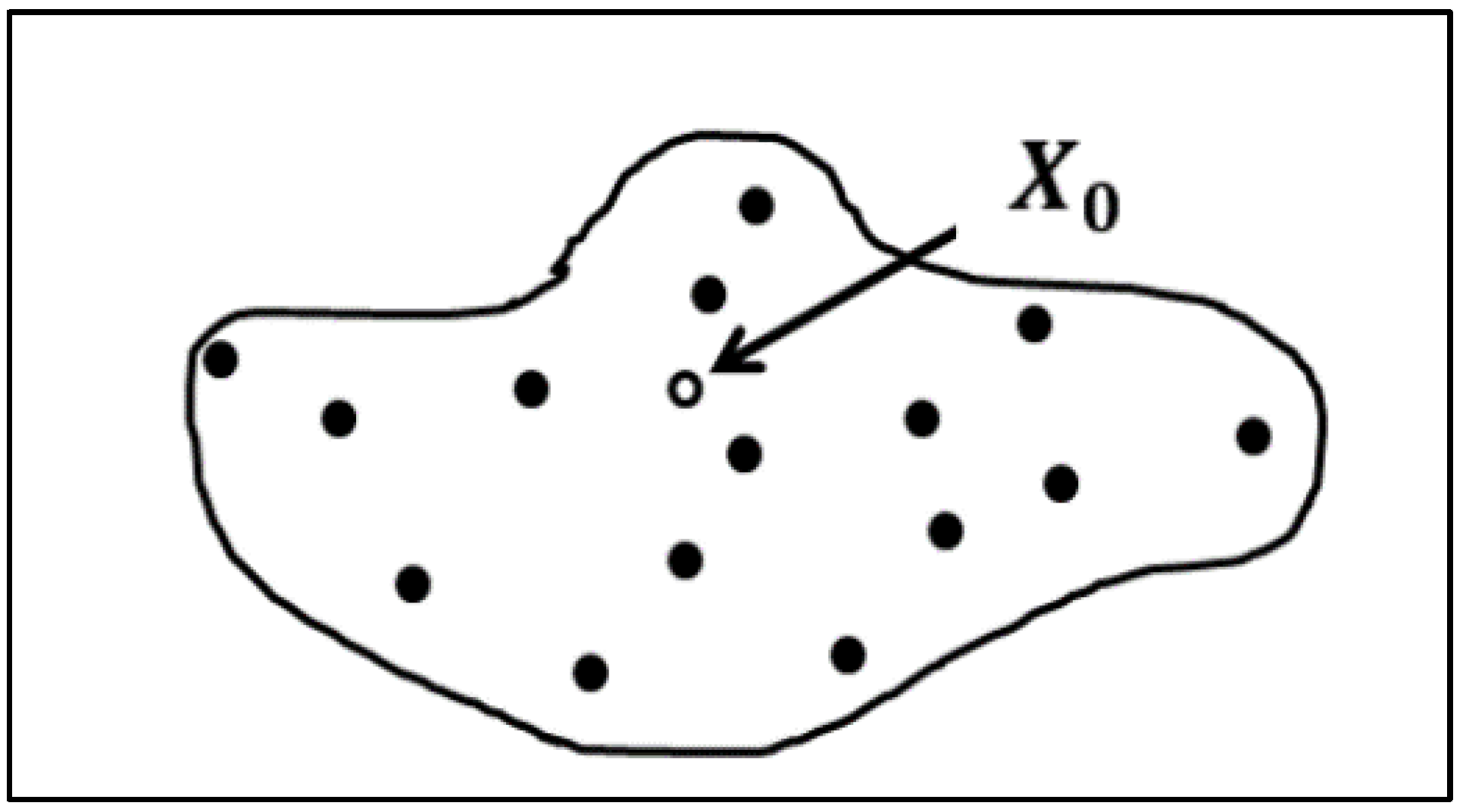
Moreover, the authors stated a few advantages of kriging models in comparison with other regression methods. Providing estimates with the mean squared error of the estimation (kriging variance), non-requirement of any distributional assumption related to the data, the ability to use a complete set of spatial and temporal information, and the ability to use a limited number of sampled data points to estimate the value of a variable over a continuous spatial field are some of them.

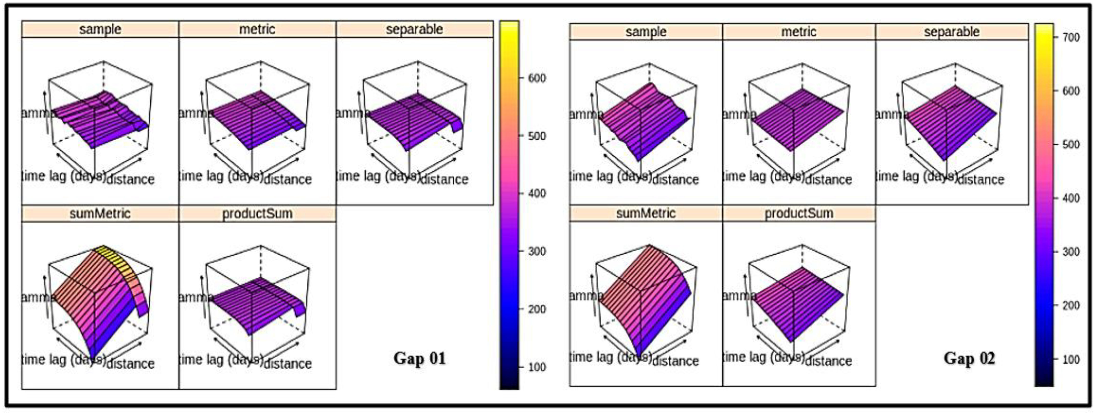
Due to these prominent advantages of kriging, recent studies have integrated kriging with conventional methods (e.g., regression and time series models) to gain fair and more accurate predictions for the missing observations. Nevertheless, a few research studies that use such hybrid approaches were found. The study [17] applied a spatiotemporal kriging method to model total monthly rainfall data among 269 rain gauge stations, of which nearly 80% of stations had missing data. The deterministic trend component was estimated with multiple linear regression, taking several covariates, including latitude, longitude, and quadratic effect of the corresponding longitude and latitude pairs. Since it only captured 29% of the temporal variability in rainfall, the residuals produced by the model were analyzed using a generalized product-sum spatiotemporal variogram and the interpolation was carried out with spatiotemporal kriging. The final predictor was obtained by combining trend estimate and interpolated value with kriging. In another study [5], spatial association of atmospheric temperature data was modeled with universal kriging and temporal variability was captured with autoregressive (AR) techniques. Then, they were spatiotemporally combined to predict k-steps (days) ahead temperature in a given spatial domain. A comparison of forecasted values with those obtained from ARIMA model indicated that the novel hybrid model performed better than the ARIMA model.

The recent advancements in machine learning (ML) and deep learning (DL) can be utilized effectively to predict missing cases in meteorological data. Both approaches have a great ability to handle large-scale problems and provide a flexible architecture in capturing spatial and temporal features [1,2]. In addition, they do not rely on hand-crafted feature engineering and prior assumptions on input data. Moreover, the aptness of deep neural networks on large volumes of spatiotemporal data compared to statistical and other classical machine learning techniques has been recognized.

A convolution bidirectional long short-term memory (LSTM) model was applied to capture spatial and temporal patterns in traffic flow data in the study [2]. This model outperformed state-of-the-art missing data imputation models. Some studies, including the study carried out in [19], demonstrated the effectiveness and efficiency of deep learning (DL) methods compared to the ARIMA model and back propagation neural network model. A convolutional neural network (CNN)-based DL model was proposed in [14] for imputing missing values in weather data of an individual weather station on a temporal basis. The performance of the model was evaluated using various stations nearest to the stations without missing values. This study used five optimizers (Rmsprop, Adam, Nadam, Stochastic Gradient Descend, (SGD), and Adagrad) and found that the SGD optimizer provides the most accurate results in predicting missing values.

Past studies reveal that the application of spatial kriging and DL methodology in missing value imputation of weather data has promising results. However, studies that impute missing values in spatiotemporal weather data using hybrid models are extremely rare, especially when there is a lower number of weather gauging stations. The existing research [5,17,20], which applies hybrid models, used more than 50 weather stations when interpolating spatiotemporal missing data. Most importantly, so far, no study has applied a spatiotemporal hybrid model to impute missing values among rainfall data at the Ratnapura gauging station. Therefore, to reduce this gap in the literature and to utilize the potential of spatial kriging, machine learning, and deep learning techniques in dealing with missing values, this study proposes a hybrid model by integrating them. Our target is to verify its appropriateness when the periods with missing values of rainfall gauging stations are different and discontinuous. Our focus is also given to the scenario where data are available only for a few rainfall stations.

The rest of this paper is organized as follows. The next section describes the adopted missing values imputation methods and the development of the new approach. The results and discussion section, followed by the conclusion are lined up last.

2. Materials and Methods

2.1. Proposed Methodology

This study introduces a hybrid method by integrating multi-layer perceptron (MLP) with spatial kriging as a tool for imputing sequential missing values of spatiotemporal data. The performance of the new model was evaluated against each of the two individual models as well as the spatiotemporal kriging model, since many past studies [17,18,20] have identified the spatiotemporal kriging model as a promising tool for estimating missing values in spatiotemporal data.

The methodology behind this study will be illustrated using the rainfall data set gathered across several neighbouring weather stations for a sufficiently longer period.

The target variable in this study represents rainfall measurements and each data point has a timestamp (day) and 2D spatial location (longitude and latitude). Our initial experiments performed for missing value imputation using machine learning methods (MLP, long short-term memory (LSTM), convolutional neural network (CNN), CNN-LSTM, ConvLSTM, random forest (RF), and nonlinear autoregressive network with exogenous inputs (NARX)) revealed that MLP can capture the temporal variation of the same set of rainfall data better than the other methods (see Table S1). Therefore, in this study, we chose MLP to capture the temporal variation of rainfall data in our hybrid model. The spatial kriging was used to model spatial variation due its promising behavior in capturing the spatial variations of the weather data and incorporation into a hybrid model [4,17,18,20,21,22].

2.1.1. Multi-Layer Perceptron Neural Network

Multi-layer perceptron (MLP) is a feed-forward neural network consisting of three types of layers: input layer, hidden layer (s), and output layer. In an MLP, the data flow in the forward direction from the input to the output layer, and the MLPs are trained with the backpropagation learning algorithm, which allows nonlinear mapping between the input and the output layer [23]. Its fast operation, ease of implementation, and requirement of a smaller training set (compared to radial basis neural networks) lead it to be popular among researchers [24].

In MLP, each neuron in a layer is connected to all neurons in the succeeding layer and connection strength is called weight. The output of each neuron of hidden layers as well as the output layer is a function of the sum of the inputs to the node modified by applying a linear or nonlinear transfer or an activation function [25,26]. The input layer passes the input vector to the network. An MLP can have one or more hidden layers.

Figure 1 illustrates an example of an MLP model with two hidden layers. Here, $X_i$ is the input to the $i^{th}$ neuron in the input layer. $w_{ij}^{\left(1\right)}$ is the weight associated with the $i^{th}$ neuron of the input layer to the $j^{th}$ neuron of the first hidden layer, $w_{ij}^{\left(2\right)}$ is the weight of the link connecting the $i^{th}$ neuron of the first hidden layer to the $j^{th}$ neuron of the second hidden layer, and $w_{ij}^{\left(3\right)}$ is the weight associated with the $i^{th}$ neuron of the second hidden layer to the $j^{th}$ neuron of the output layer. $b_i^{\left(1\right)}$ and $b_i^{\left(2\right)}$ are the bias values associated with the $i^{th}$ neuron of the first hidden layer and the $i^{th}$ neuron of the second hidden layer, respectively. $b_j$ is the bias associated with the $j^{th}$ neuron of the output layer. ${\varnothing }^{\left(1\right)}$, ${\varnothing }^{\left(2\right)}$, and ${\varnothing }^{\left(3\right)}$ are the activation functions associated with the first hidden layer, second hidden layer, and the output layer, respectively.

Then, the net output from the $i^{th}$ neuron of the first hidden layer is given by $h_i^{\left(1\right)}$ and the net output from the $j^{th}$ neuron of the second hidden layer is $h_j^{\left(2\right)}$ (see Equations (1) and (2)). The output of the $j^{th}$ neuron of the output layer will be $\widehat{y_j}$ (in our study, $j=1$). This is also noted as the imputed rainfall value at Ratnapura by MLP.

Finally, the MLP network computations can be written as follows:

$$h_i^{\left(1\right)}={\varnothing }^{\left(1\right)}\left({\sum }_j{w}_{ij}^{\left(1\right)}{X}_{i }+b_j^{\left(1\right)}\right) \mathrm{w}\mathrm{h}\mathrm{e}\mathrm{r}\mathrm{e} i=1, 2, 3 \mathrm{a}\mathrm{n}\mathrm{d} j=1, 2, 3, 4$$

(1)

$$h_j^{\left(2\right)}={\varnothing }^{\left(2\right)}\left({\sum }_i{w}_{ij}^{\left(2\right)}{h}_i^{\left(1\right)}+b_i^{\left(2\right)}\right) \mathrm{w}\mathrm{h}\mathrm{e}\mathrm{r}\mathrm{e} i=1, 2, 3, 4 \mathrm{a}\mathrm{n}\mathrm{d} j=1, 2, 3$$

(2)

$$\widehat{{\mathit{y}}_{\mathit{j}}}={\varnothing }^{\left(3\right)}\left(\sum _i{w}_{ij}^{\left(3\right)}{h}_j^{\left(2\right)}+b_j\right) \mathrm{w}\mathrm{h}\mathrm{e}\mathrm{r}\mathrm{e} i=1, 2, 3 \mathrm{a}\mathrm{n}\mathrm{d} j=1$$

(3)

2.1.2. Spatial Kriging

Spatial kriging is an optimal interpolation technique that uses the theory of regression to predict the value at an unobserved location using values of observed neighborhood locations. Here, observed values of neighborhood locations are weighted according to the covariance values. As depicted in Figure 2, consider the location of interest, $X_0,$ that is surrounded by the neighboring observed locations, $X_i$.

The value at location $X_0$, ${Z(X}_0)$, is estimated through the values of $n$ neighboring sample locations taken as a linear combination of observed location values. Let the weight be associated with the observed value at location $X_i$, i.e., ${Z(X}_i)$ is $w_i$. Then, the spatial kriging estimate of ${Z(X}_0)$ can be computed as follows:

$$\widehat{Z}\left(X_0\right)=k+\sum _{i=1}^n{w}_{i}Z\left(X_i\right)=k+w^T\mathit{Z}$$

(4)

where $w \equiv {\left(w_1, w_2, \dots , w_n \right)}^T,\mathit{Z} \equiv \left(Z\left(X_1\right), Z\left(X_2\right), \dots , Z\left(X_n\right)\right)$. The values of $k$ and $w$ are calculated by minimizing the mean squared prediction error [18].

The optimal linear predictor of ${Z(X}_0)$, ${\widehat{\mathit{Z}}(\mathit{X}}_0),$ is given by:

$${\widehat{\mathit{Z}}(\mathit{X}}_0)=\mu \left(X_0)+{\mathit{c}}^T{\sum }^{-1}(\mathit{Z}-\mathit{\mu }\right)$$

(5)

where $\mu$ is the Lagrange multiplier, $\mathit{\mu }\equiv {(\mu \left(X_1\right),\mu \left(X_2\right),\dots ,\mu \left(X_n\right))}^T$, $\left(X_i\right)=E\left(Z\left(X_i\right)\right)$, $i=0,1,2,\dots ,n$, $\mathit{c}\equiv {(Cov\left(X_0,X_1\right),\dots ,Cov\left(X_0,X_n\right))}^T$, and $\sum$ is the $n\times n$ matrix whose $\left(i,j\right)$^th element is $Cov\left(X_i,X_j\right)$.

Then, the minimum value of $MSE\left(X_0, w, k\right)$ for a fixed location $X_0$, ${\sigma }^2\left(X_0\right)$ (spatial kriging variance) is given by [18]:

$${\sigma }^2\left(X_0\right)=Cov\left(X_0, X_0\right)-{\mathit{c}}^T{\sum }^{-1}\mathit{c}$$

(6)

The values of $\mathit{c}$ and $\sum$ are calculated through the variogram or a covariance function. The different kriging models (simple, ordinary, or universal) can be obtained by changing the way of modeling $E\left(Z\left(X\right)\right)$.

2.1.3. Hybrid Model for Missing Value Estimation

In the proposed hybrid model, the spatial kriging estimate and the MLP estimate are integrated with optimal weights. The optimal weights must be estimated using a sample of artificially created missing cases. Suppose the spatial kriging estimate of that sample is ${\widehat{y}}_k$ (which was produced as ${\widehat{Z}(X}_0)$ in Section 2.1.2) and the MLP estimate is ${\widehat{y}}_m$ (which was produced as $\widehat{y_j}$ in Section 2.1.1), weights from each estimate are $w_k$ and $w_m$, respectively, the actual value is $y_a$, and the final estimate is ${\widehat{y}}_f$. In order to find the final prediction closer to the actual value, the optimal weights from each prediction should be found such that the prediction error is minimized. Therefore, the optimization problem can be defined as mean squared error (MSE) loss function ($f_{loss}$) between predicted and actual values:

$$f_{loss}\left(w_k, w_m\right)=\sum _{i=1}^n{\left(w_k{\widehat{y}}_{ki}+w_m{\widehat{y}}_{mi}-y_{ai}\right)}^2$$

(7)

with respect to the following constraints that provide a convex combination of two edge points ${\widehat{y}}_{ki}$ and ${\widehat{y}}_{mi}$:

$$w_k+w_m=1, {0\le w}_{k }\le 1, 0{\le w}_m\le 1$$

(8)

Following the study [27], it would be logical to consider the case when the weights $w_k$ and $w_m$ are greater than 1 or less than 0. Considering this assumption and denoting ${w=w}_k$, Equations (7) and (8) can be formulated as an unconstrained optimization problem with respect to $w$ in the form:

$$\mathrm{M}\mathrm{i}\mathrm{n}\mathrm{i}\mathrm{m}\mathrm{i}\mathrm{z}\mathrm{e}: f_{loss}\left(w\right)={\sum }_{i=1}^n{\left(w {\widehat{y}}_{ki}+(1-w) {\widehat{y}}_{mi}-y_{ai}\right)}^2$$

(9)

The objective function $f_{loss}\left(w\right)$ in this problem is convex and smooth; therefore, optimization Equation (9) can be easily solved. We have:

$$\frac{1}{dw} f_{loss}\left(w\right)=\sum _{i=1}^{n}2\left(w {\widehat{y}}_{ki}+(1-w) {\widehat{y}}_{mi}-y_{ai}\right)({\widehat{y}}_{ki}-{\widehat{y}}_{mi})=0$$

(10)

Solving Equation (10) with respect to $w$, we find optimal weight $w$ and, therefore, weights $w_{k }=w$ and $w_m$ in the form:

$$w_k=\left({\sum }_{i=1}^n\left({{\widehat{y}}_{mi}}^2+{\widehat{y}}_{ki}{y}_{ai}-{\widehat{y}}_{mi}{y}_{ai}-{\widehat{y}}_{ki}{\widehat{y}}_{mi}\right)\right)/\left({\sum }_{i=1}^n\left({{\widehat{y}}_{ki}}^2+{{\widehat{y}}_{mi}}^2-2{\widehat{y}}_{ki}{\widehat{y}}_{mi}\right)\right)$$

(11)

$$\mathrm{a}\mathrm{n}\mathrm{d}\hspace{1em}{w}_m=1-w_k$$

(12)

The found optimal weights were used to obtain the final prediction $\widehat{{\mathit{y}}_{\mathit{f}}}$ at the point $i$ where the particular value is missing:

$${\widehat{\mathit{y}}}_{\mathit{f}}=w_m\ast {\widehat{y}}_m+w_k\ast {\widehat{y}}_k$$

(13)

The imputed missing values using the proposed method were compared with those obtained from spatial kriging, MLP as well as spatiotemporal kriging. The reason for considering spatiotemporal kriging is that it is a widely used spatiotemporal missing value imputation method in past studies.

2.1.4. Spatiotemporal Kriging

The spatial kriging can be extended to obtain spatiotemporal predictions by incorporating an additional temporal dimension, $t$, to the spatial kriging [4,17,18,20].

The spatiotemporal set of observed data are given by $\left\{{Z(X}_1, t_1), {Z(X}_2, t_2), \dots , {Z(X}_n, t_n)\right\}$, and let $Z_i={Z(X}_i, t_i)$ be the value of the variable $Z$ at location $X_i$ and time $t_i$. The spatiotemporal kriging prediction at an unobserved location $X_0$ at time $t$ is defined by:

$${\widehat{\mathit{y}}}_{\mathit{f}}=\widehat{Z}(X_0, t)={\sum }_{i=1}^n{w}_i(X, t)\left(Z\right(X_i, t_i\left)\right) \mathrm{s}\mathrm{u}\mathrm{b}\mathrm{j}\mathrm{e}\mathrm{c}\mathrm{t} \mathrm{t}\mathrm{o}{\sum }_{i=1}^n{w}_i(X, t)=1$$

(14)

where $w_i$ are weights for ${Z(X}_i, t_i), i=1, 2, \dots n$. Following the study in [18], the optimal prediction is taken by minimizing the mean squared prediction error subject to the constraint:

$$E\left[{\widehat{Z}(X}_0, t)-Z(X_0, t)\right]=0$$

(15)

The kriging weights can be computed through the covariance function or by means of a semivariogram. Once the covariance values are calculated, the optimal weights of the kriging estimator can be computed through Lagrange multiplier application. Finally, the optimal value of ${\widehat{Z}(X}_0, t)$ is calculated for spatiotemporal location ${(X}_0, t)$ [18].

The spatiotemporal covariance function has different models such as linear, exponential, spherical, Gaussian, or logistic. Capturing the spatial and temporal variability is difficult for the variogram due to their dissimilarities. Therefore, the two-dimensional kriging is modified to incorporate the time component. The type of variogram (metric, separable, SumMetric, and product sum models) varies according to the way it combines and models the temporal and spatial dependencies. The best-fitting model can be identified by comparing the mean squared errors (MSE) between the sample variogram and fitted variogram.

2.1.5. Model Evaluation

In order to evaluate the performance of the fitted MLP, spatial kriging and spatiotemporal kriging models, mean absolute error ($MAE$), root mean squared error ($RMSE$), and coefficient of determination ($R^2$) metrics were used.

The $MAE$, $RMSE$, and $R^2$ are calculated as below.

$$MAE=\frac{1}{n} \sum _{i=1}^n\left|y_{ai}-{\widehat{y}}_{fi}\right|$$

(16)

$$RMSE=\sqrt{\frac{1}{n} \sum _{i=1}^n{\left(y_{ai}-{\widehat{y}}_{fi}\right)}^2}$$

(17)

$$R^2=1-\frac{{\sum }_{i=1}^n{\left(y_{ai}-{\widehat{y}}_{fi}\right)}^2}{{\sum }_{i=1}^n{\left(y_{ai}-{\overline{y}}_{ai}\right)}^2}$$

(18)

where ${\widehat{y}}_{fi}$ is the predicted value, $y_{ai}$ is the actual value, and ${\overline{y}}_{ai}$ is the mean value of $y_{ai}$. The smaller the values of MAE and RMSE and larger the $R^2$ value, the better the forecasting is.

The hybrid model, which integrates MLP and spatial kriging, was implemented in python and the spatiotemporal kriging model was fitted using R software (version 4.3) and the related packages. In the spatiotemporal model, the data were represented as Space Time Full Data Frame (STFDF) object before fitting the variogram since data considered in this study were with complete space time grid with s substations and t time intervals of their observations.

2.2. Description of Data

For this study, daily rainfall readings gathered by nine rainfall neighbouring gauging stations, including the target station (Ratnapura), were considered. The other eight stations are Balangoda (St1_Bal), Detanagalla (St2_Det), Elston (St3_Els), llumbuluwa (St4_Ill), Keragala (St5_Ker), Moralioya (St6_Mor), Nivithigala (St7_Niv), and Ulinduwawa (St8_Uli). These eight stations are considered as reference stations.

The total number of days accounted for in this study is 1826. As mentioned earlier, these reference stations consist of various discontinuous missing patterns within the study period (1 January 2015–31 December 2019). The following heatmap (Figure 3) depicts the missing patterns in the data of eight reference stations and

Table 1. Missing percentages of sub-stations’ rainfall data.

Sub Station	Missing Count	Missing Percentage
St1_Bal	32	1.75
St2_Det	1	0.05
St3_Els	519	28.42
St4_Ill	491	26.89
St5_Ker	123	6.74
St6_Mor	183	10.02
St7_Niv	1249	68.4
St8_Uli	1343	73.55

summarizes percentages.

Figure 3 depicts the data availability with blue color and inconsistent missingness with white blocks along the time and space. With respect to the figure, it can be noted that, in most cases, the missingness has occurred as a block (i.e., a sequence of missing values). The percentage of missing values of the last two sub-stations, as indicated in Table 1, are 68.4% and 73.55%, respectively. Since more than half of the data values are missing, these two sub-stations were excluded from the analysis. The stations St1_Bal, St2_Det and St5_Ker had random missing cases (noncontinuous missing values). Those were interpolated using the average values of the neighbouring rainfall values of the corresponding station. Finally, there were six reference stations considered for assessing the suitability of the proposed methodology.

3. Results and Discussion

3.1. Preliminary Analysis

The correlation between the rainfall values of different stations may be either linear or nonlinear. Therefore, to capture any type of correlations, the Spearman correlation coefficients were calculated (refer to Figure 4).

The correlation between all the considered sub-stations and the target station Ratnapura and among sub-stations are significant at 5% significance level (i.e., $p$ value $<0.05$). A strong correlation ($>0.6$) can be seen between Ratnapura and sub-stations Keragala, Moralioya, and Elston. The results indicate that all six sub-stations are important in modeling rainfall at Ratnapura station. Thus, it confirms the need for imputing missing values of the reference stations.

3.2. The Hybrid Model Formation

The structure of the performed hybrid model with MLP and spatial kriging can be depicted as in Figure 5. In the notation, ${\widehat{\mathit{y}}}_{\mathit{k}}$ and ${\widehat{\mathit{y}}}_{\mathit{m}}$ refers to the spatial kriging and the MLP estimates corresponding to the missing rainfall value of the $i^{th}$ station, for instance, St2 (there are situations where the rainfall values of more than one station are missing on the same day).

Note that MLP (for multivariate time series data) was trained using the parameter values tuned with grid search approach (selected from a range of values) tabularized in

Table 2. Common parameter settings in MLP models.

Parameters	Value
Activation function	ReLU
Epochs	80
Number of hidden layers	1
Number of neurons in hidden layer	20
Batch size	72
Learning rate	0.01
Optimizer	Adam
Loss Function	MAE

.

The regularization parameters and number of training/testing samples were modified to obtain a convergent model in each MLP model. As depicted in Figure 5, in order to integrate the two estimates obtained from spatial kriging and MLP, the optimal weights from each estimate should be found.

For this, a data set without missing values needs to be used. Therefore, the following procedure was applied:

(a)

From the original data set, three complete subsets (with no missing cases for all the stations) were selected. Consequently, subsets from the years 2015, 2016, and 2019 were selected.

(b)

Consecutive missing periods were artificially created randomly within the three subsets to capture the missing pattern of the original data set.

(c)

The spatial kriging and MLP were applied to estimate the missing cases.

(d)

Those estimated rainfall values were combined to form a single data set of 120 estimated rainfall values.

(e)

Then, from the final data set mentioned in (d), 100 simple random samples (with replacement) with a moderate sample size of 60 were drawn.

(f)

For each sample, the optimal values of two weights, $w_k$ and $w_m,$ were calculated by applying Equations (11) and (12) as described in Section 2.1.3. The procedure resulted in 100 optimal pairs of weights.

(g)

Then, the first optimal weight pair was used to calculate the weighted estimates (${\widehat{\mathit{y}}}_{\mathit{f}}$) of the rest of the samples (99). For each sample, the RMSE values (including the first sample considered) were calculated. Using these RMSE values, the average RMSE was computed.

(h)

Likewise, steps (a) to (g) were repeated using the second optimal weight pair, then third optimal weight pair, and so on.

Finally, there were 100 average RMSE values. Out of them, the pair of weights that produced the lowest average RMSE value was selected as the best optimal pair of weights for spatial kriging and MLP (Table S2). The results indicated that the 11th random sample produced the final optimal weights, $w_k=0.50013$ and ${ w}_m=0.49987$. Those weights were taken to obtain optimal weighted estimates for the missing values.

3.3. The Spatiotemporal Kriging Model (SPTK Model)

Figure 6 summarizes the steps followed in applying the spatiotemporal kriging model.

In this approach, a variogram for each missing sequence was fitted using the available rainfall values of stations. For example, according to Figure 6, the first gap of the above data set can be seen in station St2. Then, the data from the remaining stations were employed to fit a variogram. Similarly, the missing blocks of St4 and St6 were estimated using the available rainfall values of the other stations and so on.

Four variogram types (metric, separable, sum metric, and product sum) were compared in terms of RMSE values. Using the variogram with the lowest RMSE, the spatiotemporal kriging was applied to estimate the missing values in a substation(s) that was/were in the created grid.

Table 3. Comparison of prediction errors of variogram types.

Gap no	Metric	Separable	SumMetric	Product Sum
1	13.79	23.16	64.75	23.33
2	38.56	22.871	52.43	22.868
3	15.46	16.19	31.14	16.25
4	30.31	30.86	71.54	30.82
5	136.15	132.79	128.77	132.79
6	17.53	10.03	31.8	9.99
7	11.02	9.67	9.13	9.66
8	88.75	89.13	110.29	89.28
9	21.58	21.95	41.33	22.13
10	81.02	81.03	118.85	81.04
11	34.95	13.54	58.8	13.63

provides the outputs resulting from 11 blocks of missing values.

According to Table 3, it can be noticed that, in most of the cases, the metric variogram has become the best fit and Figure 7 depicts a sample of figures (out of 11 figures), which illustrates the comparison between variograms. In each case, the sample variogram and fitted four types of variograms are given.

In fitting the spatiotemporal model for the rainfall data, the empirical variogram surface (or sample variogram) based on space and time is computed and used as inputs for fitting different models: metric, separable, sum metric, and product sum models. Out of them, the best fitting model can be selected, comparing with the surface of the empirical variogram. When considering Missing Gap 01 in Figure 7, the metric-type variogram shows the most similar surface shape with respect to distance and time lags as that of the original sample. Nevertheless, in Missing Gap 02, the product sum variogram is more similar to the pattern of the actual sample. Likewise, in 11 gaps, the optimal variogram type deferred with the missing pattern of the data.

Through optimal variograms the covariances of the data were calculated and, thereby, the optimal weights to predict the missing value at the targeted location (see Section 2.1.4).

3.4. Model Evaluation

To validate the models, a two-way evaluation mechanism was carried out.

3.4.1. Model Evaluation along with Actual Missing Data

Assume that the rainfall values of a station are missing from $t$ to $t+k_1$ (see Figure 8). The hybrid model was fitted, and these missing values were estimated using the available values from $1$ to $t$. To check the validity of the fitted model, rainfall values from ($t+k_1$) to ($t+k_1+k_2$) were estimated based on the same fitted model (refer to Section 3.2) and compared with the actual values. This validation data set was with size 55 (here, the total number of observations in all $k_2$ periods). The value $k_2$ was chosen according to the continuous availability of data within the considered time period.

Spatiotemporal kriging (SPTK) was applied to the same validation set. Finally, a comparison of RMSE, MAE, and R² (

Table 4. Comparison of prediction error of all models.

Method	Spatial Kriging	MLP	Hybrid	SPTK
RMSE	12.76	11.68	10.72	15.97
MAE	7.12	4.01	5.12	10.25
R2	13%	3%	13%	0%

) was conducted using the results produced by individual approaches and the hybrid approach.

Among the considered four models, the minimum RMSE is produced by the hybrid weighted method. It also has an MAE close to its lowest value, which is produced by MLP, and the highest R² value as of the spatial kriging (although it still needs to be improved). Thus, in the first phase of model comparison, it was proved that the hybrid model outperformed the other individual models. Moreover, the hybrid model outperformed the spatiotemporal kriging model with respect to all validation measurements.

3.4.2. Model Evaluation on Artificially Generated Missing Data

Since the previous evaluation could not capture all the actual missing gaps (due to the inconsistency of the data set), we thought to generalize the validation using another validation set that could capture all the missing patterns (which are and are not in the original data set) that could be found in an original data set of six rainfall gauging stations.

In year 2016, for 6 months (from January to June), there were no missing observations. Therefore, we took the data of that period to create 56 subsets with different sequential missing patterns, as shown in

Table 5. Types of missing gaps within six sub-stations.

Number Stations with Missing Observations (M)	Number of Combinations (of Stations)
01	6C1 = 6
02	6C2 = 15
03	6C3 = 20
04	6C4 = 15
Total number of data sets	56

.

When two stations have missing observations in the same period (consider one incident out of 15 combinations in case 02), each station was modeled separately. Thus, it resulted in two trials. Finally, all combinations of two stations with missing observations (i.e., 15) generated 30 trials (15 × 2). This was the same for the rest of the cases where there were at least two stations with missing data. The case where the number of stations with missing observations, M = 5, was not considered because there should be at least two stations without missing observations in the spatiotemporal grid to model those gauging stations with missing values using spatial kriging (a model requirement). In each subset, missingness was created with the last 20 observations (without breaking the time sequence and allocating enough data points for training) of the relevant sub-station. The rest of the data were used to train and test the models and, hence, identify the best-fit model for a selected sample of data.

The estimated values from each model were compared with the actual values and tabularized in Table S3. In terms of the lowest values of RMSE and MAE and the highest values of R², the hybrid model has outperformed the other approaches. Moreover, it is important to point out that, when kriging performs better than other individual methods in terms of three validation measurements, the hybrid model has performed approximately equally in most of the cases.

The outperformance with respect to the total (where lowest RMSE and MAE values and highest R² value occur) shows the hybrid method could gain the score of 41% (see

Table 6. Final comparison of model performance.

Method	Kriging	MLP	Hybrid	SPTK
No. of times that each approach produced best results (as a percentage with respect to the sum of trials)	30	20	41	9

).

In addition to the above outcome, all the cases (in Table S3) were taken to obtain the graphs shown in Figure 9.

Figure 9 illustrates that kriging produced most cases within the lowest value range of MAE and within the highest value range of R², whereas the MLP gained the majority of cases within the lowest value range of RMSE. In all these occurrences, the hybrid model has shown approximately the same performance as the optimal model.

This study demonstrated that the spatial and temporal variations should not be neglected in missing value imputation in spatiotemporal data. Further, considering the two-way evaluation, we could confirm that the hybrid model had the ability to outperform other pure approaches or almost equally performed compared to the best approach whenever it was selected as the second-best approach.

4. Conclusions

In this paper, we proposed a novel approach for spatiotemporal missing value imputation. Furthermore, this approach was illustrated by applying it to impute rainfall data in six reference stations to compile a complete data set that could be used in building a rainfall forecasting model for a target station. The proposed approach is a hybrid approach combining MLP that captures the temporal variability and spatial interpolation (spatial kriging) that captures the spatial variations. This hybrid model was designed for imputing missing values when the missingness of reference stations was spread discontinuously and not uniformly over the given period and a few rainfall gauging stations are spatially correlated. Moreover, the results obtained by the hybrid model were compared with those resulting from spatiotemporal kriging. The study supported the claim that the proposed hybrid approach provided the lowest prediction error when estimating a sequence of missing values.

Only a single published research study that imputes the missing rainfall values of Ratnapura gauging stations is available. The accuracy measurements of the proposed method are far better than those of said study [28].

The availability of a few rain gauging stations around Ratnapura station and unavailability of data in some stations for a considerable period due to relocation or other reasons were the challenging limitations confronted during this study.

In order to verify the optimality of weight estimates and the outperformance of the hybrid method, the data for an extended period need to be gathered and tested.

While considering the aforesaid limitations, the future direction of this research will be the development of more hybrid models combining other missing value imputation methods and applying this approach to estimate missing values of spatiotemporal data obtained from other fields.

References

1. Mital, U.; Dwivedi, D.; Brown, J.B.; Faybishenko, B.; Painter, S.L.; Steefel, C.I. Sequential Imputation of Missing Spatio-Temporal Precipitation Data Using Random Forests. Front. Water 2020, 2, 20. [Google Scholar] [CrossRef]
2. Asadi, R.; Regan, A. A convolution recurrent autoencoder for spatio-temporal missing data imputation. arXiv 2019, arXiv:1904.12413. [Google Scholar]
3. Soley-Bori, M. Dealing with Missing Data: Key Assumptions and Methods for Applied Analysis; Boston University: Boston, MA, USA, 2013; Volume 4, pp. 1–19. [Google Scholar]
4. Yang, H.; Yang, J.; Han, L.; Liu, X.; Pu, L.; Chin, S.; Hwang, H. A Kriging based spatiotemporal approach for traffic volume data imputation. PLoS ONE. 2018, 13, e0195957. [Google Scholar] [CrossRef] [PubMed]
5. Agarwal, A. A New Approach to Spatio-Temporal Kriging and Its Applications. Master’s Thesis, Ohio State University, OhioLINK Electronic Theses and Dissertations Center, Columbus, OH, USA, 2011. Available online: http://rave.ohiolink.edu/etdc/view?acc_num=osu1306871646 (accessed on 18 November 2023).
6. Aguilera, H.; Guardiola-Albert, C.; Hidalgo, C.S. Estimating extremely large amounts of missing precipitation data. J. Hydroinformatics 2020, 22, 578–592. [Google Scholar] [CrossRef]
7. Feng, L.; Nowak, G.; O’Neill, T.J.; Welsh, A. CUTOFF: A spatio-temporal imputation method. J. Hydrol. 2014, 519, 3591–3605. [Google Scholar] [CrossRef]
8. Hettiarachchi, P. Inundation Maps of the Kalu Ganga Basin during the Flood in May 2003; Department of Irrigation: Colombo, Sri Lanka, 2013. [Google Scholar]
9. Nandalal, K.D.W. Use of a hydrodynamic model to forecast floods of Kalu River in Sri Lanka. J. Flood Risk Manag. 2009, 2, 151–158. [Google Scholar] [CrossRef]
10. Rafii, F.; Kechadi, T. Collection of historical weather data: Issues with missing values. In Proceedings of the 4th International Conference on Smart City Applications (SCA’19), Casablanca, Morocco, 2–4 October 2019. [Google Scholar]
11. Burhanuddin, A.; Zahrah, S.N.; Deni, S.; Ramli, N.M. Imputation of Missing Rainfall Data Using Revised Normal Ratio Method. Adv. Sci. Lett. 2017, 23, 10981–10985. [Google Scholar] [CrossRef]
12. Jahan, F.; Sinha, N.; Rahman, M.; Rahman, M.M.; Mondal, M.S.; Islam, M. Comparison of Missing Value Estimation Techniques in Rainfall Data of Bangladesh. Theor. Appl. Climatol. 2019, 136, 1–17. [Google Scholar] [CrossRef]
13. Ahmad, R.; Noor, F.; Zakaria, R.; Azman, M.A. Estimation of missing rainfall data using spatial interpolation and imputation methods. AIP Conf. Proc. 2015, 1643, 42–48. [Google Scholar] [CrossRef]
14. Gad, I.; Doreswamy, H.; Manjunatha, B. A robust deep learning model for missing value imputation in big NCDC dataset. Iran J. Comput. Sci. 2021, 4, 67–84. [Google Scholar] [CrossRef]
15. Afrifa-Yamoah, E.; Mueller, U.; Taylor, S.; Fisher, A. Missing data imputation of high-resolution temporal climate time series data. Meteorol. Appl. 2020, 27, e1873. [Google Scholar] [CrossRef]
16. Nassir, S.; Badr, A.; Mousa, W. Estimation the Missing Data of Meteorological Variables in Different Iraqi Cities By using ARIMA Model. Iraqi J. Sci. 2018, 59, 792–801. [Google Scholar]
17. Medeiros, E.; De Lima, R.; Olinda, R.; Santos, C. Modeling Spatiotemporal Rainfall Variability in Paraíba, Brazil. Water 2019, 11, 1843. [Google Scholar] [CrossRef]
18. Cuenca, J.; Correa-Flórez, C.; Patino, D.; Vuelvas, J. Spatio-Temporal Kriging Based Economic Dispatch Problem Including Wind Uncertainty. Energies. 2020, 13, 6419. [Google Scholar] [CrossRef]
19. Duan, Y.; Lv, Y.; Liu, Y. An efficient realization of deep learning for traffic data imputation. Transp. Res. Part C Emerg. Technol. 2016, 72, 168–181. [Google Scholar] [CrossRef]
20. Zoest, V.V.; Osei, F.; Hoek, G.; Stein, A. Spatio-temporal regression Kriging for modelling urban NO2 concentrations Spatio-temporal regression Kriging for modelling urban NO2 concentrations. Int. J. Geogr. Inf. Sci. 2019, 34, 851–865. [Google Scholar] [CrossRef]
21. Bae, B.; Kim, H.; Lim, H.; Liu, Y.; Han, L.; Freeze, P. Missing data imputation for traffic flow speed using spatio-temporal cokriging. Transp. Res. Part C Emerg. Technol. 2018, 88, 124–139. [Google Scholar] [CrossRef]
22. Srinivasan, B.; Duraiswami, R.; Murtugudde, R. Efficient Kriging for real-time spatio-temporal interpolation. In Proceedings of the 20th Conference on Probability and Statistics in the Atmospheric Sciences, Atlanta, Georgia, 18–21 January 2010; p. 228. [Google Scholar]
23. Abirami, S.P.; Chitra, P. Chapter Fourteen-Energy-efficient edge based real-time healthcare support system. Adv. Comput. 2020, 117, 339–368. [Google Scholar]
24. Orhan, U.; Hekim, M.; Ozer, M. EEG signals classification using the K-means clustering and a multilayer perceptron neural network model. Expert Syst. Appl. 2011, 38, 13475–13481. [Google Scholar] [CrossRef]
25. Gardner, M.W.; Dorling, S.R. Artificial neural networks (the multilayer perceptron)—A review of applications in the atmospheric sciences. Atmos. Environ. 1998, 32, 2627–2636. [Google Scholar] [CrossRef]
26. Grosse, R. Lecture 5: Multilayer Perceptrons. 2018. Available online: https://www.cs.toronto.edu/~rgrosse/courses/csc321_2018/readings/L05%20Multilayer%20Perceptrons.pdf (accessed on 16 January 2022).
27. Zhou, Y.; Guan, Z.; Ji, P.; Wang, X. Drug Abuse Prediction Model Based on Relevance Analysis. In Data Processing Techniques and Applications for Cyber-Physical Systems (DPTA 2019)–Advances in Intelligent Systems and Computing; Huang, C., Chan, Y.W., Yen, N., Eds.; Springer: Singapore, 2020; Volume 1088. [Google Scholar] [CrossRef]
28. Jeewanthi, P.W.; Wijesuriya, W.; Liyanarachchi, L.A.T.S.; Gunatathne, L.H.P. Appropriate conventional methods forestimating missing precipitation values in Sri Lanka. J. Agric. Value Addit. 2023, 5, 45–53. [Google Scholar] [CrossRef]
Figure 1. A multilayer perceptron model with two hidden layers. The nodes in Input Layer are represented in green colour. The nodes in Hidden Layer are represented in blue colour, and the node in Output Layer is coloured in red.
Applsci 14 00999 g001
Figure 2. The neighboring observed locations and the location of interest, X 0 .
Applsci 14 00999 g002
Figure 3. Missing patterns of sub-stations’ rainfall data.
Applsci 14 00999 g003
Figure 4. The heatmap of correlation between rainfall gauging stations.
Applsci 14 00999 g004
Figure 5. The hybrid model structure.
Applsci 14 00999 g005
Figure 6. The spatiotemporal kriging method.
Applsci 14 00999 g006
Figure 7. Differences between the sample and the best fitting spatiotemporal variogram of each family of the first two gaps. The half of the variogram function (γ—gamma) which gives measures of spatiotemporal correlation of the random field is plotted against each space–time co-ordinate.
Applsci 14 00999 g007
Figure 8. The model evaluation criterion.
Applsci 14 00999 g008
Figure 9. The outperformance of models with respect to RMSE (a), MAE (b), and R2 (c) values.
Applsci 14 00999 g009