Biogas Production Prediction Based on Feature Selection and Ensemble Learning

Abstract

The allocation of biogas between power generation and heat supply in traditional kitchen waste power generation system is unreasonable; for this reason, a biogas prediction method based on feature selection and heterogeneous model integration learning is proposed for biogas production predictions. Firstly, the working principle of the biogas generation system based on kitchen waste is analyzed, the relationship between system features and biogas production is mined, and the important features are extracted. Secondly, the prediction performance of different individual learner models is comprehensively analyzed, and the training set is divided to reduce the risk of overfitting by combining K-fold cross-validation. Finally, different primary learners and meta learners are selected according to the prediction error and diversity index, and different learners are fused to construct the stacking ensemble learning model with a two-layer structure. The experimental results show that the research method has a higher prediction accuracy in predicting biogas production, which provides supporting data for the economic planning of kitchen waste power generation systems.

1. Introduction

Unlike coal, oil, natural gas, and other energy sources, biomass energy has the characteristics of a low energy flow density and a wide range of sources, making it suitable for building combined heat and power systems with a high energy utilization efficiency and significant economic benefits [1]. Biomass energy is of great significance in the process of promoting the low carbon development of power systems [2]. However, the accuracy and efficiency of the data analysis are affected by the many dimensions and complexity of the data from new energy systems, such as wind power, photovoltaic, and biomass [3]. Thanks to the rapid development of artificial intelligence technology, more machine learning algorithms have been applied to the field of electric energy [4]. Artificial intelligence and machine learning algorithms, such as back propagation (BP) neural network models [5], eXtreme Gradient Boosting (XGBoost) [6], recurrent neural networks (RNN) [7], support vector machines (SVM) [8], and other methods, are widely used in the research of renewable energy forecasting and load forecasting.

The above methods are only a single technique used in data prediction, and there is still a lot of room for improvement in the prediction problem. In order to avoid the problem of poor generalization performance due to the randomness of a single model, much research has used combinatorial models. Qu et al. [9] designed a multi-step prediction model by stacking bagging, long short-term memory (LSTM), and random forest (RF) algorithms together, and obtained relatively accurate wind power prediction results. Pan et al. [10] used a combined model approach to fuse the light gradient boosting machine (LightGBM), RF, and SVM algorithms with stacking ensemble models to achieve high recall and accuracy in the classification problem. Liu et al. [11] used a stacking model to fuse multiple XGBoost models and used a two-layer stacking prediction model to maximize the performance of XGBoost, which achieved better results on short-term bus load prediction data, but the prediction results on biogas data were poor, and further analysis of the ensemble model is needed to improve the prediction accuracy.

Aiming at the problem that existing algorithms are not accurate in predicting biogas production, the biogas power generation system studied in this paper centers on the biogas produced by the fermentation of kitchen waste, and proposes a biogas prediction method from the physical state data of each part of the gas production system. The specific contributions are as follows:

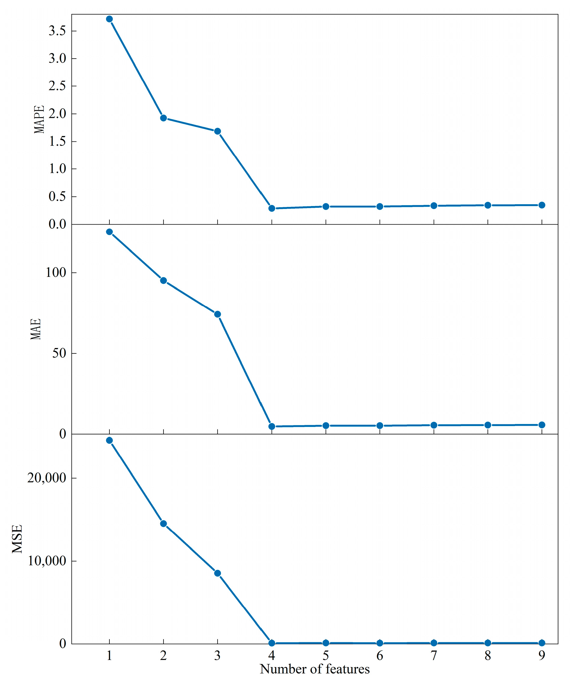
• We analyze the correlation coefficients between system features and target features, combine the working principle of the system, screen out the features with strong correlation, and obtain the optimal number of input model features based on the preliminary prediction.
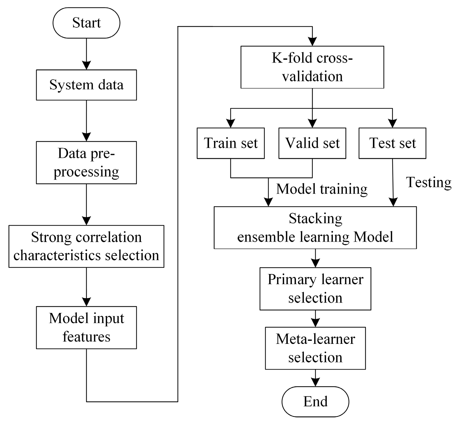
• We use the K-fold cross-validation method to divide the dataset proportionally to avoid the overfitting problem.
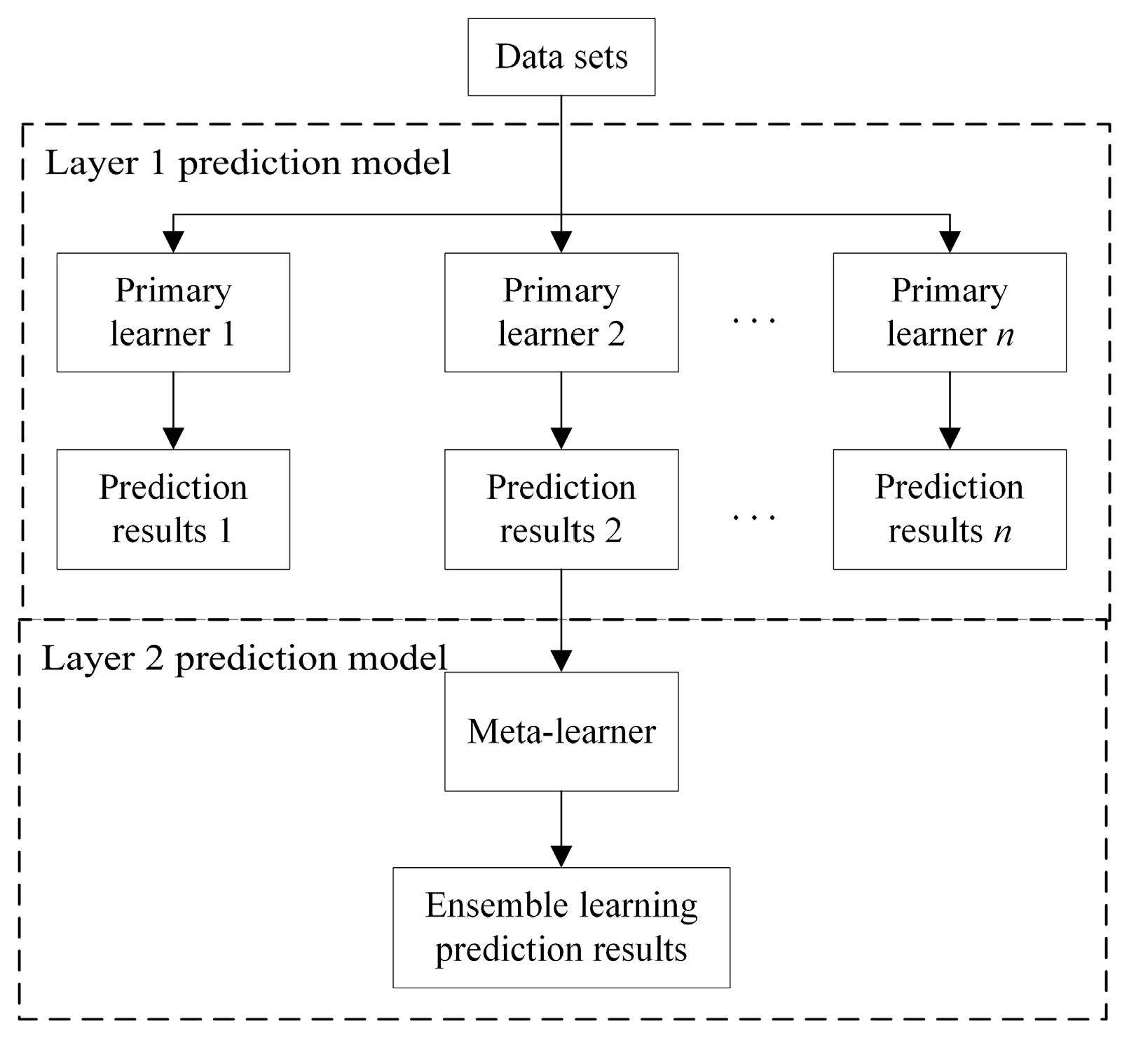
• A stacking ensemble learning model is constructed based on different models for training and prediction, and the stacking model with the best prediction effect is obtained under different base learners and meta learners.

The paper is structured as follows: In Section 2, the kitchen waste power system studied in this paper is introduced, and the structure of the proposed biogas prediction model is described in detail. In Section 3, the actual operational data of the kitchen waste system is used for experiments and the results are presented and discussed. In Section 4, the conclusion is presented.

2. Materials and Methods

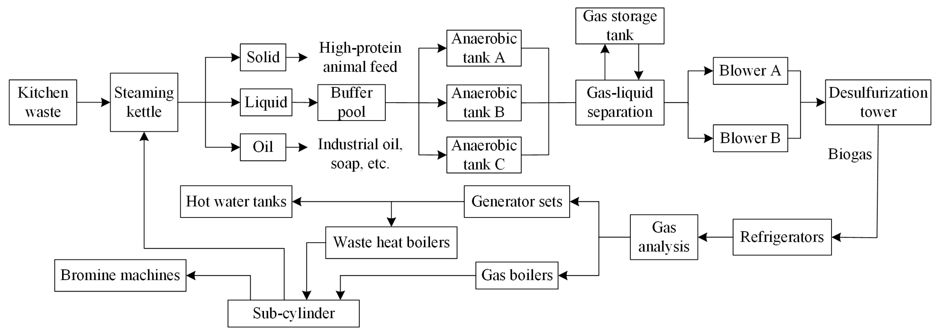
2.1. Biogas Power Generation Systems

2.1.1. System Introduction

Food scraps and garbage produced in families, restaurants, and other places, known as kitchen waste, can be harmful to the environment if not handled properly [12]. Studies have shown that kitchen waste contains a variety of energy sources, such as carbohydrate polymers, which can be used for renewable energy production [13]. The kitchen waste power generation system is based on the multi-energy complementary technology of coupling cold, heat, electricity, and gas multi-energy streams, and uses information and communication technology to collaboratively dispatch controllable energy sources to achieve safe and stable operation of the system [14]. The kitchen waste power generation system studied in this paper uses anaerobic fermentation to produce biogas. Anaerobic digestion technology is environmentally friendly and has the advantages of low carbon emissions, low operating costs, low secondary pollution, and is suitable for large-scale centralized treatment. It is of great significance in the process of achieving carbon peaking and carbon neutrality. The energy system for achieving the harmless treatment of kitchen waste with biogas power generation is shown in Figure 1. The system collects and treats food waste produced by major catering industries and centralizes it for harmless treatment. The specific processing steps are: kitchen waste is entered into the system and is cooked by steam in the cooking kettle to separate the solid, liquid, and oil in the waste wastewater. The oil is processed into industrial oil and soap raw materials. The solid waste is used as high protein animal feed. The liquid separates into the buffer tank and finally ferments in the anaerobic tank to produce biogas. The biogas enters the biogas generator set and gas boiler after dehydration, desulfurization, and cooling. The biogas is used in the generator to generate electricity for production purposes, and in the boiler system to produce heat and steam to meet its own production conditions.

2.1.2. The Necessity of Biogas Production Forecasting

At the present stage, the biogas power generation system lacks a link to a biogas production prediction, and the distribution of biogas between the boilers and the generator sets relies on manual experience. In order to further improve the construction of biogas-based Internet of Things and to improve the control and energy efficiency of the power generation system [15], it is necessary to forecast the biogas output. At the same time, the analysis and prediction of the internal characteristics of the system are a key prerequisite for the collaborative system scheduling, and the accuracy of the prediction affects the economy and reliability of the system scheduling. The main manifestations are: the production activities in the steaming kettle are driven by steam, and the demand for steam should be matched with the amount of steam generated by the boiler to achieve the synergistic cooperation of all parts of the system, and improper control will result in an unnecessary waste of energy. Workers control the input of raw materials to the system by switching on and off the waste water tank, and a lack of consideration of the relationship between the internal demand of the boiler and the biogas production will lead to a reduction in the energy efficiency of the system. The production of biogas as a key part in these problems affects the generation of electricity by the generator and heat production by the boiler, as well as the amount of steam that subsequently enters the steaming kettle. The production of biogas is closely related to the allocation of system resources and the energy utilization rate, so an accurate prediction of the biogas production is the main prerequisite for rational resource allocation and the maximization of benefits.

2.1.3. Feature Selection

The kitchen waste power generation system consists of a water and gas treatment part, a generator system and a boiler system, which contains many kinds of data, but the information expressed by each data source is limited, and not all data sources provide value for the model. If all influencing factors are taken as the input of the model, it will lead to a complex model structure and reduce the model performance. Therefore, feature selection is used to find the data that can really affect the objective function, and then the input and output of the model are reasonably selected to determine the structure of the model to include as much valuable information as possible [16].

In order to explore the relationship between the features and biogas production, the filter feature selection method [17,18] is used to calculate the correlation by the two-dimensional vector Pearson correlation coefficient, and the features with stronger correlations are retained. The Pearson correlation coefficient indicates the linear relationship between the data, representing the linear correlation between two variables x and y, expressed by r. The value of r is between −1 and 1, and the larger its absolute value, the stronger the correlation. Its calculation formula is shown in Equation (1):

$$r=\frac{{\displaystyle \sum _{i=1}^m(x_i-\overline{x})(y_i-\overline{y})}}{\sqrt{{\displaystyle \sum _{i=1}^m{(x_i-\overline{x})}^2}}\sqrt{{\displaystyle \sum _{i=1}^m{(y_i-\overline{y})}^2}}}$$

(1)

where $r$ is the Pearson correlation coefficient, $x_i$ and $y_i$ is a pair of continuous correlation variables, and $\overline{x}$ and $\overline{y}$ are, respectively, the mean values of the variables $x$ and $y$.

Sorting by the size of correlation coefficient, the features with a large absolute value of the correlation coefficient are selected as strong correlation features. Then, a different number of features are selected for prediction, and an error curve based on the number of features is obtained. From this, the number of features to be input into the final model is determined, and the extraction of important features is completed [19].

A total of 79 characteristics are chosen from the three components of the kitchen waste power generation system. Combined with the analysis in Figure 1, it can be seen that of the three components, biogas production is more correlated with the water and gas treatment part. Twenty-one features of the water and gas treatment part are selected for analysis, among which, the operating frequency and frequency setting features of the two blowers do not change during system operation, while the change in the pressure regulating value feature is directly reflected in the inlet pressure features. Therefore, the correlation between the remaining 15 characteristics and the biogas production are discussed. Specific correlation coefficient calculations are shown in

Table 1. System features and correlation coefficient.

System Features	Correlation Coefficient with Biogas Production
Anaerobic tank: Inlet main line pressure	0.1994
Anaerobic tank: Outlet main line pressure	0.1731
Blower A: Inlet pressure	−0.3835
Blower A: Current	0.3130
Blower B: Inlet pressure	−0.3152
Blower B: Current	0.3143
Anaerobic tank A: Pressure	−0.0471
Anaerobic tank A: Water inlet	0.2837
Anaerobic tank A: Gas flow rate	0.6860
Anaerobic tank B: Pressure	−0.0414
Anaerobic tank B: Water intake	0.2999
Anaerobic tank B: Gas flow rate	0.7231
Anaerobic tank C: Pressure	0.1121
Anaerobic tank C: Water inlet	0.3270
Anaerobic tank C: Gas flow rate	0.6860

. The retained features are selected based on the data in Table 1, and the specific selection process is described in Section 3.2.

2.1.4. Prediction Model Structure

The flow chart of the biogas prediction model studied in this paper is shown in Figure 2, and the research method adopted has the following characteristics: (1) the working principle of the biogas system is analyzed for the features of water and gas treatment systems with a high correlation to ensure the correlation and validity of the model input features; (2) the optimal number of model input features is determined based on the preliminary prediction results to simplify the model structure; (3) the K-fold cross-validation is used to alleviate the overfitting problem of the model; (4) a combination of many different single methods is analyzed to select the best combination of learners using an error and a Pearson correlation index to build the stacking ensemble learning model, which further improves the prediction accuracy of the model.

2.2. Biogas Prediction Based on Heterogeneous Ensemble Learning

An ensemble learning algorithm is a meta-algorithm that accomplishes the learning task by combining multiple algorithms together, which itself does not belong to a separate machine learning algorithm [20]. Currently, based on different learning purposes, ensemble learning algorithms mainly include bagging algorithms with minimum output variance, a boosting algorithm with minimum deviation, and a stacking algorithm with an improved forecasting effect. In ensemble learning, choosing the best combination strategy can avoid the problem of low generalization in a single learner. For the regression problem, the more common combination strategies are averaging and learning. The averaging method includes simple averaging and weighted averaging, but the averaging method simply combines the prediction results obtained by the learners, assigning the corresponding weights to each learner by some specific conditions, without effectively using the data space [21]. The learning method is to learn the results further by another learner, of which the stacking algorithm is a representative of the learning method.

2.2.1. Stacking Ensemble Learning Algorithm

The purpose of the stacking algorithm is to train and build a model for combining other models. In general, stacking ensemble learning with a two-layer structure can enhance the learning effect and simplify the model [22,23]. The learner in the first layer is the primary learner, and the learner in the second layer is the meta-learner. The basic idea is as follows: firstly, the data is divided into a training set, a validation set, and a test set, and the K-fold cross-validation method is used to train the primary learner from the original dataset. Then, the output obtained from the primary learner is combined as features with the corresponding tokens of the initial training set to form a new dataset for training the meta-learner. In this way, the diversity among different learners is preserved and the learning effect is strengthened by the different learning strategies. The structure of the two-layer stacking ensemble learning is shown in Figure 3.

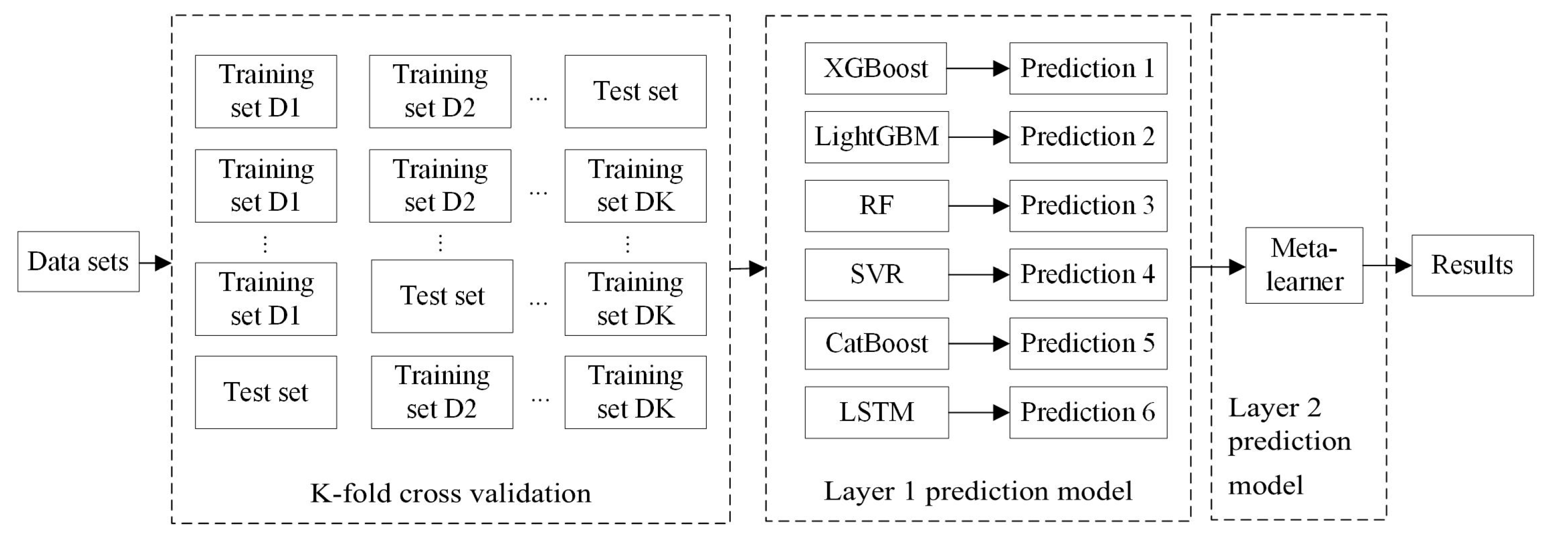
2.2.2. K-Fold Cross-Validation

Generally, in model evaluation, the data is divided into a training set, a validation set, and a test set, and then the data set is put into the model for training, and the data from the test set is input into the model after training, and the results obtained will be used to judge the merits of the model. If the trained model gets a small error in the training set and a large error in the test set, it indicates that the model is overfitting. In stacking ensemble learning, the data used to train the primary and meta-learner may lead to a higher risk of overfitting if they are duplicated. The reason for overfitting is that the tuning process of model hyperparameters relies on the performance of the validation set on the model as feedback, and each tuning will leak more information into the model, and multiple cycles of this process will cause the model to be overfitted on the test set. In order to effectively avoid the impact of information leakage on the model and reduce the risk of overfitting the model, K-fold cross-validation is used. The training set is randomly divided into K subsets of the same size, and when training the model, each subset is selected in turn as the test set, while the other K-1 subsets are used as the training set. The number of training tests for each learner is K, and the result of the last K tests is used as the final return value.

In K-fold cross-validation, the value of K is generally $2\le K\le 10$, and the specific value is shown in Equation (2).

$$\left\{\begin{array}{l}K\approx \ln N\\ N/K>3d\end{array}\right.$$

(2)

where N is the total number of samples and d is the number of features.

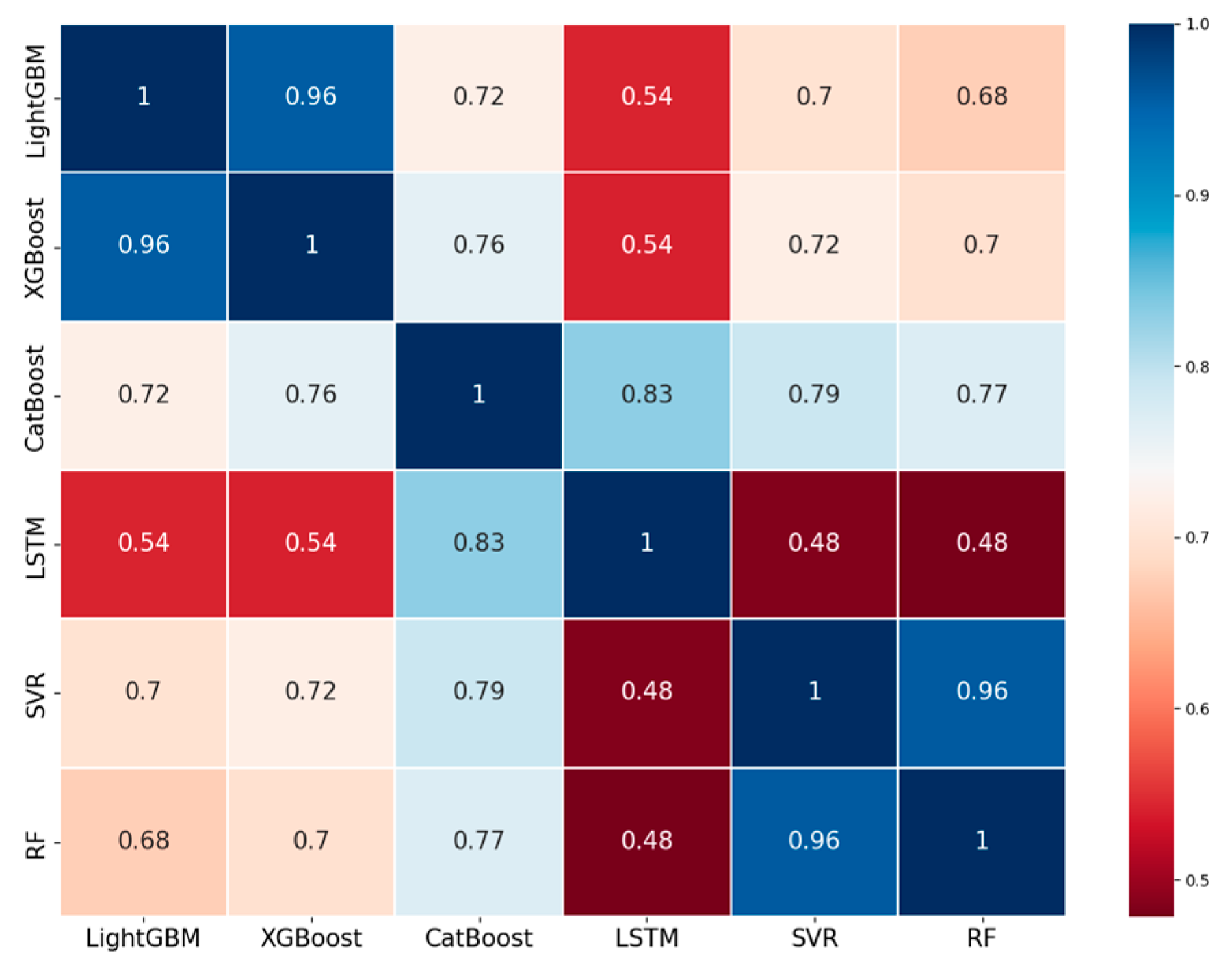
2.2.3. Construction of the Heterogeneous Ensemble Learning Model

For the regression problem, the prediction performance of the learner is the starting point, and the selection of a model with a strong learning ability helps to improve the overall prediction effect of the model. LSTM, SVR (support vector regression), RF, XGBoost, LightGBM, and CatBoost (gradient boosting and categorical features) are chosen as the first layer learners in the stacking model. Among them, the single learner LSTM has a mature theory and good practice, and is widely used. SVR is an important application branch of SVM, which uses a support vector in performing the fitting and a Lagrange multiplier style to analyze the data regression. RF uses the ensemble learning method of bagging. XGBoost, LightGBM, and CatBoost use the ensemble learning method of boosting. These methods have found wide application and practice in various fields. In order to prevent the model from overfitting on the training set, the selection of the second layer stacking model should not be too complicated, and a model with a strong generalization ability and simplicity should be selected. In summary, LSTM, SVR, RF, XGBoost, LightGBM, and CatBoost are initially selected as primary learners, and XGBoost, LightGBM, and CatBoost as meta-learners. The biogas prediction model based on model fusion stacking ensemble learning is shown in Figure 4.

Further, different models are built from different data perspectives and the algorithmic principles of the models themselves. For the first layer of primary learners, while considering the prediction performance, in order to obtain a better fusion model effect and give full play to the advantages of different models, the complementary characteristics between the different models need to be considered, that is, there needs to be certain differences between models. The stacking model relies on the differences between sub models to maximize the advantages of the integration algorithm [24].

2.2.4. Evaluation Metrics

In order to verify the prediction effect of heterogeneous ensemble learning, the two-dimensional vector Pearson correlation coefficient is used as an analytical evaluation index to comprehensively analyze the distribution of prediction errors among the different primary learners. By calculating the Pearson correlation coefficient of the errors generated by the prediction between each primary learner, the learners with larger differences are then filtered as the primary learners of the stacking model.

The prediction accuracy and performance of the prediction models are mainly evaluated by the error between the predicted value and the true value, and the main evaluation indexes are the MSE (mean squared error), the MAE (mean absolute error), and the MAPE (mean absolute percentage error). The MSE is used to detect the deviation of the predicted value from the true value and has a better interpretation, and the larger the value is, the larger the prediction error is. The MAE reflects the mean of the absolute error, which can better reflect the actual situation of the error of the predicted value. The formulas for calculating the correlation error are as follows:

$$MSE=\frac{1}{n}{\displaystyle \sum _{i=1}^n{({\widehat{y}}_i-y_i)}^2}$$

(3)

$$MAE=\frac{1}{n}{\displaystyle \sum _{i=1}^n\left|{\widehat{y}}_i-y_i\right|}$$

(4)

$$MAPE=\frac{100\%}{n}{\displaystyle \sum _{i=1}^n\left|\frac{{\widehat{y}}_i-y_i}{y_i}\right|}$$

(5)

where ${\widehat{y}}_i$ is the predicted biogas yield, $y_i$ is the actual biogas yield, and n is the length of the predicted biogas yield series.

3. Results and Discussion

3.1. Data Sets

The analyzed data are selected from a science and technology project using multi-energy complementary cooling, heating, and power technology based on kitchen waste with an intelligent management system. The real-time sampling values of the operating data from the system from 1 to 23 May 2022 are selected as the raw data, with a sampling interval of 5 min to predict the biogas production in the coming week. The raw data contains a total of 79 data characteristics from three parts of the kitchen waste power generation system, as well as final biogas production data and power generation data.

3.2. Feature Analysis

XGBoost is used to make a preliminary prediction of the biogas production. The features with the top ranked Pearson correlation coefficients are selected as the most influential features, and then different numbers of features are selected for prediction to obtain the error curve based on the number of features. The number of features is determined based on the error curve, and Figure 5 shows the change curve of the XGBoost model’s error for different numbers of features.

As can be seen from Figure 5, when the number of selected features is greater than or equal to 4, the error curve decreases significantly. Therefore, it is determined that four features should be selected as input to the data. Combined with the data in Table 1, in this paper, the gas flow rate of the three anaerobic tanks and the inlet pressure of blower A are selected as the basic features, and the absolute values of their Pearson correlation coefficients with the biogas production are 0.6860, 0.7231, 0.6860, and 0.3835, respectively. Taking these four features as inputs to the model improves the prediction effect and reduces the complexity of the model.

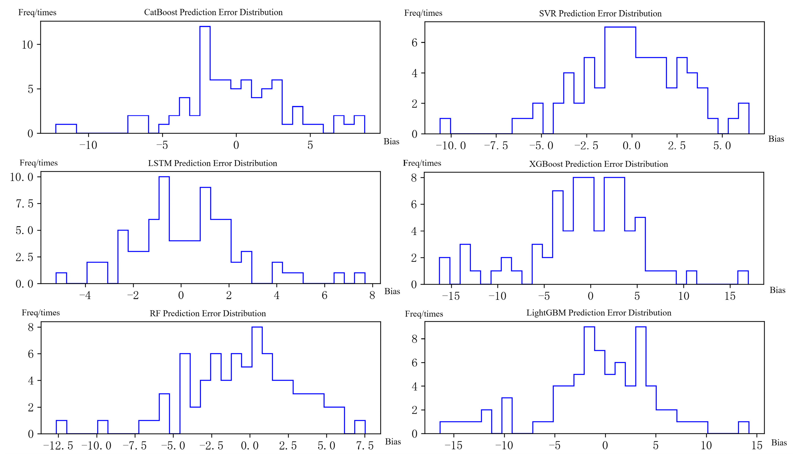
3.3. Individual Learner Prediction Performance Analysis

The prediction analysis of each weak learner is performed before building the stacking model, and LightGBM, XGBoost, CatBoost, RF, SVR, and LSTM models are selected to analyze the learning ability of each model and the degree of correlation between models. The pre-processed data combined with the cross-validation method are predicted separately on each base learner. Figure 6 shows the histogram comparison of the error frequency distribution for each algorithm predicted separately, with the horizontal coordinate being the prediction error and the vertical coordinate being the frequency of error occurrence.

As can be seen from Figure 6, the overall prediction error frequency distribution of CatBoost is concentrated in the interval [−5, 5] when each learner model independently predicts the biogas yield. CatBoost is improved under the gradient boosting decision tree (GBDT) [25] algorithm with a symmetric decision tree as the base learner, and the indexes of the leaf nodes on each layer of the decision tree are encoded as binary vectors with a length equal to the tree depth, which improves the prediction speed while being less prone to overfitting. Considering that the biogas production data is a set of time-series data, the biogas generation is not only related to the production state input at the current moment, but also related to the past input features. An LSTM neural network can make full use of the data information from a past time, so the LSTM prediction error is also relatively small, and most of the errors are concentrated in the [−4, 5] interval. There are small outliers in the prediction structure of other models, and these outliers reduce the prediction effectiveness.

In order to screen the best model as the primary learner, the distribution among the errors obtained by each base learner’s individual prediction is compared. The diversity among the models is examined while considering the prediction effect, and the Pearson correlation coefficient index is used to analyze the degree of variation among the models. Figure 7 shows the LightGBM, XGBoost, CatBoost, RF, SVR, and LSTM based learners’ prediction error correlation metrics on the original dataset.

From Figure 7, it can be seen that the error correlation is higher for LightGBM, XGBoost, and CatBoost. This is because they are all representative algorithms based on boosting, they all belong to the ensemble algorithms of decision trees, and there is a certain degree of similarity in their way of processing data. The error correlation is lower for the neural network-based LSTM model, SVR, and RF. This is because there are some differences in the mechanism of data training among these methods. In summary, CatBoost, LSTM, SVR, and RF, having lower error correlations, are selected as primary learners.

3.4. Meta-Learner Selection

The meta-learner of the stacking model can reduce the risk of overfitting while improving the deviation of various types of learners and enhance the generalization ability of the model. To verify the feasibility of the model proposed in this paper to predict biogas production, the meta-learner is selected as XGBoost, LightGBM, and CatBoost models to verify the prediction effectiveness of different meta-learners.

Table 2. Evaluation metrics for the different meta-learner stacking models.

Meta-Learner	MSE	MAE	MAPE
XGBoost	74.489	3.658	0.220
CatBoost	80.054	3.699	0.223
LightGBM	86.994	4.709	0.238
LSTM	107.86	5.07	0.3022
RF	98.64	4.21	0.2520
SVR	118.03	5.19	0.3244

shows the prediction performance of different meta-learners on the stacking model.

From Table 2, the stacking fusion model has been improved to some extent in its bio-gas prediction effect compared with the single model, and when the meta-learner is selected as XGBoost, the stacking model has the lowest error with an MSE of 74.489 and an MAE of 3.658. The stacking fusion model studied in this paper has a learner configuration of CatBoost, LSTM, SVR, and RF as the primary learners and XGBoost as the meta-learner in a two-layer stacking structure, so as to maximize the accuracy of the biogas production prediction.

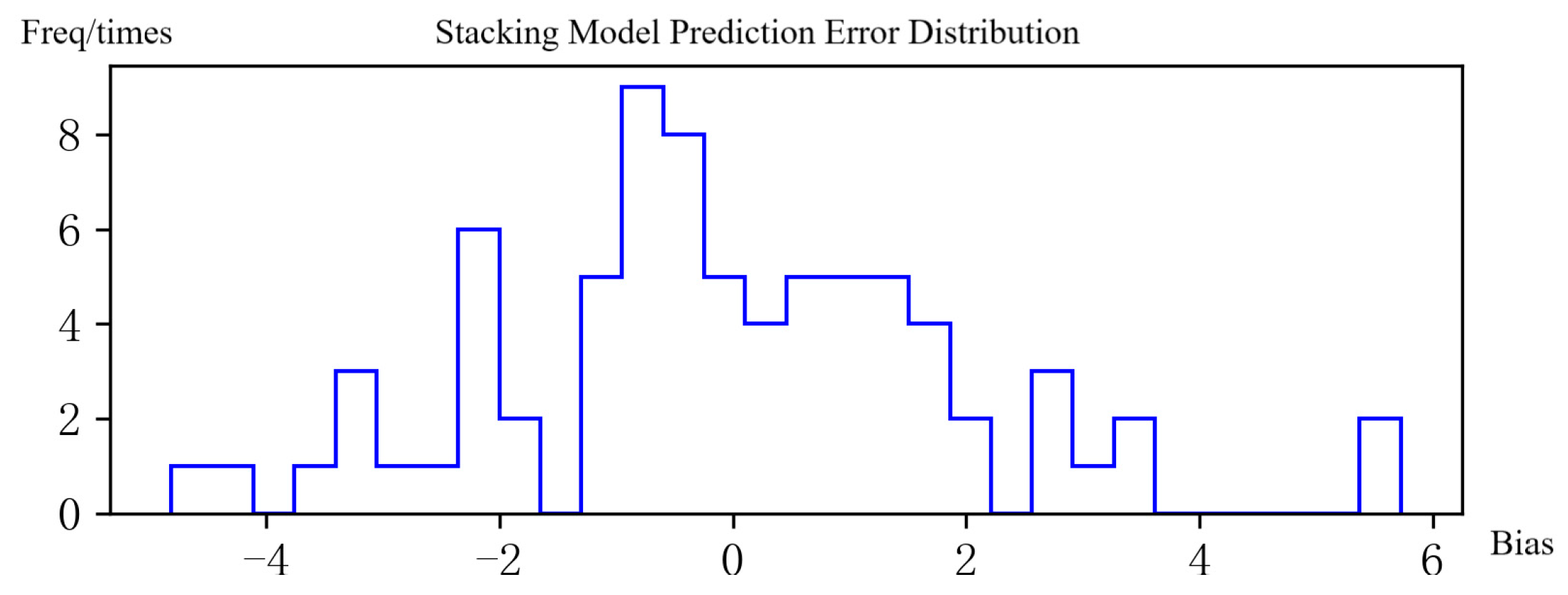
3.5. Prediction Performance Analysis

Theoretically, the stacking ensemble model should have a lower prediction error than a single model. This is because the stacking model combines the strengths of multiple primary learners and the combined strategy based on the learning method learns the data further on the meta-learner for better results. As a result, the stacking model improves the poor generalization performance of the data using a single model. At the same time, during the model training process, there is a situation where a single model falls into local minima. However, the stacking ensemble model can effectively reduce the risk of falling into local minima by combining the operating effects of multiple models. In summary, the stacking ensemble model improves the prediction accuracy and model generalization ability.

To further assess the impact of the variability among primary learners on the overall prediction effect of the stacking model, the prediction errors of the stacking model for other combinations of primary learners are given in

Table 3. Evaluation metrics for different combinations of primary learners.

Model	Primary Learner Set	Average Error Correlation Coefficient	MSE	MAE	MAPE
Model 1 (proposed method)	CatBoost, LSTM, SVR, RF	0.68	74.489	3.658	0.220
Model 2	CatBoost, LightGBM, XGBoost, SVR	0.86	117.08	4.72	0.280
Model 3	CatBoost, LightGBM, LSTM, SVR	0.745	84.54	4.63	0.224
Model 4	LightGBM, XGBoost, LSTM, RF	0.8	104.97	4.20	0.254
Model 5	CatBoost, XGBoost, LSTM, SVR	0.755	98.61	4.03	0.242

. The meta-learner of each model in Table 3 is XGBoost, and the combination of models with a high correlation of different Pearson errors is chosen. The average error correlation coefficient is the average of the error Pearson correlation coefficients between the meta-learner and the primary learner. Model 1 is the best combination of primary learners obtained from the previous analysis.

From Table 3, different combinations of primary learners have a certain degree of influence on the overall prediction effect of the stacking ensemble model. The lower the average error correlation coefficient is, the smaller the prediction error of the obtained model. So, choosing a less correlated learner as the primary learner can make the prediction performance of the stacking ensemble learning model better. There are two reasons for this analysis: choosing the learner with a smaller error for integration can improve the overall prediction ability of the ensemble model; and different models are trained to process the data from different perspectives, so choosing the model with greater variability as the primary learner can give full play to the advantages of different models and improve the prediction effect of the stacking ensemble model. Figure 8 shows the histogram of the prediction error distribution obtained by the proposed method. After comparing Figure 8 with Figure 6, the prediction error of the stacking ensemble learning model is concentrated in the interval [−4, 4], and the overall prediction accuracy is higher than that of a single method.

4. Conclusions

In this paper, a biogas prediction model based on feature selection and heterogeneous ensemble learning is proposed and applied to the prediction of biogas in anaerobic tanks in biogas power generation systems for the problem of ensemble planning and rational resource allocation. The correlation between the internal features of the system and the biogas production is analyzed, while different single-prediction models are trained and tested, and the variability of different primary learner combinations and the influence of meta-learners on the prediction performance of the model are comprehensively analyzed and compared. The results show that the prediction model gives full play to the advantages of different learners, improves the accuracy of the prediction model, more accurately responds to the change trend of system parameters, solves the problem of optimal results from a single model being difficult to obtain, and provides data support for the reasonable allocation of system resources and optimization of system structure in biogas power generation systems. In the future, the research on the number of primary learners selected can be continued in the prediction model selection to further optimize the prediction performance.

References

1. Zhu, Y.L.; Wang, Y.Z.; Zhang, X.J.; Li, W.Y.; Li, J.; Li, H.J. Thermo-economic analysis of biomass-fired organic Rankine cycle combined heat and power system. Acta Energiae Solaris Sin. 2021, 42, 312–319. [Google Scholar] [CrossRef]
2. Zhang, X.H.; Liang, J.X.; Zhao, C.M.; Wang, L.; Hu, J.L.; Zhong, J.Q. Research on low-carbon power planning with gas turbine units based on carbon transactions. Acta Energiae Solaris Sin. 2020, 41, 92–98. [Google Scholar]
3. Li, Y.; Xiao, Z.Q.; Nie, S.S.; Cao, J.W.; Hua, H.C. Review of research on generative adversarial network and its application in new energy data quality. South. Power Syst. Technol. 2020, 14, 25–33. [Google Scholar] [CrossRef]
4. Ju, P.; Zhou, X.X.; Chen, W.J.; Yu, Y.P.; Qin, C.; Li, R.M.; Wang, C.S.; Dong, X.Z.; Liu, J.; Wen, J.Y.; et al. “Smart Grid Plus” research overview. Electr. Power Autom. Equip. 2018, 38, 2–11. [Google Scholar] [CrossRef]
5. Zhu, J.Q.; Niu, X.F.; Xiao, X.B. Prediction models of the carbon content of fly ash in a biomass boiler based on improved BP neural networks. Renew. Energy Resour. 2020, 38, 150–157. [Google Scholar]
6. Xiong, X.; Guo, X.J.; Zeng, P.L.; Zou, R.L.; Wang, X.L. A short-term wind power forecast method via XGBoost hyper-parameters optimization. Front. Energy Res. 2022, 10, 905155. [Google Scholar] [CrossRef]
7. Lu, J.X.; Zhang, Q.P.; Yang, Z.H.; Tu, M.F.; Lu, J.J.; Peng, H. Short-term load forecasting method based on CNN-LSTM hybrid neural network model. Autom. Electr. Power Syst. 2019, 43, 131–137. [Google Scholar] [CrossRef]
8. Xing, Y.Q.; Xing, X.J.; Zhang, J.; Li, Y.L.; Zhang, X.F.; Zhang, X.W. A prediction model of biomass three-components contents based on machine learning and thermogravimetric analysis. Acta Energiae Solaris Sin. 2019, 40, 1330–1337. [Google Scholar]
9. Qu, Z.J.; Li, J.; Hou, X.X.; Gui, J.L. A D-stacking dual-fusion, spatio-temporal graph deep neural network based on a multi-integrated overlay for short-term wind-farm cluster power multi-step prediction. Energy 2023, 281, 128289. [Google Scholar] [CrossRef]
10. Pan, G.B.; Gong, M.B.; He, M.; Wu, C.H.; Tang, X.Q.; Yang, L.; OuYang, J. Identification method of electricity charge recovery risk of specialized transformer user based on Stacking model fusion. Electr. Power Autom. Equip. 2021, 41, 152–160. [Google Scholar] [CrossRef]
11. Liu, B.; Qin, C.; Ju, P.; Zhao, J.B.; Chen, Y.X.; Zhao, J. Short-term bus load forecasting based on XGBoost and stacking model fusion. Electr. Power Autom. Equip. 2020, 40, 147–153. [Google Scholar] [CrossRef]
12. Barik, S.; Paul, K.K. Potential reuse of kitchen food waste. J. Environ. Chem. Eng. 2017, 5, 196–204. [Google Scholar] [CrossRef]
13. Jiang, J.F.; Li, L.H.; Cui, M.C.; Zhang, F.G.; Liu, Y.X.; Liu, Y.H.; Long, J.Y.; Guo, Y.F. Anaerobic digestion of kitchen waste: The effects of source, concentration, and temperature. Biochem. Eng. J. 2018, 135, 91–97. [Google Scholar] [CrossRef]
14. Yuan, J.H.; Yuan, Z.Y.; Ou, X.M. Modelling of environmental benefit evaluation of energy transition to multi-energy complementary system. Energy Procedia 2019, 158, 4882–4888. [Google Scholar] [CrossRef]
15. Lautert, R.R.; Brignol, W.D.; Canha, L.N.; Adeyanju, O.M.; Garcia, V.J. A flexible-reliable operation model of storage and distributed generation in a biogas power plant. Energies 2022, 15, 3154. [Google Scholar] [CrossRef]
16. Liu, H.; Chen, C. Data processing strategies in wind energy forecasting models and applications: A comprehensive review. Appl. Energy 2019, 249, 392–408. [Google Scholar] [CrossRef]
17. Zheng, Y.F.; Li, Y.; Wang, G.; Chen, Y.P.; Xu, Q.; Fan, J.H.; Cui, X.T. A novel hybrid algorithm for feature selection based on whale optimization algorithm. IEEE Access 2019, 7, 14908–14923. [Google Scholar] [CrossRef]
18. Akogul, S. A novel approach to increase the efficiency of filter-based feature selection methods in high-dimensional datasets with strong correlation structure. IEEE Access 2023, 11, 115025–115032. [Google Scholar] [CrossRef]
19. Zhang, D.D.; Chen, B.A.; Zhu, H.Y.; Goh, H.H.; Dong, Y.X.; Wu, T.M. Short-term wind power prediction based on two-layer decomposition and BiTCN-BiLSTM-attention model. Energy 2023, 285, 128762. [Google Scholar] [CrossRef]
20. Wang, Y.; Gu, Y.; Ding, Z.; Li, S.N.; Wan, Y.; Hu, X.R. Charging demand forecasting of electric vehicle based on empirical mode decomposition-fuzzy entropy and ensemble learning. Autom. Electr. Power Syst. 2020, 44, 114–121. [Google Scholar] [CrossRef]
21. Zhou, Z.H. Ensemble Methods: Foundations and Algorithms; CRC Press: Boca Raton, FL, USA, 2012; pp. 67–95. [Google Scholar]
22. Shi, J.Q.; Zhang, J.H. Load forecasting based on multi-model by stacking ensemble learning. Proc. CSEE 2019, 39, 4032–4042. [Google Scholar] [CrossRef]
23. Deng, W.; Guo, Y.X.; Li, Y.; Zhu, L.; Liu, D.G. Power losses prediction based on feature selection and stacking integrated learning. Power Syst. Prot. Control 2020, 48, 108–115. [Google Scholar] [CrossRef]
24. You, W.X.; Li, Q.Q.; Yang, N.; Shen, K.; Li, W.W.; Wu, Z.L. Electricity theft detection based on multiple different learner fusion by stacking ensemble learning. Autom. Electr. Power Syst. 2022, 46, 178–186. [Google Scholar] [CrossRef]
25. Friedman, J.H. Greedy function approximation: A gradient boosting machine. Ann. Stat. 2001, 29, 1189–1232. [Google Scholar] [CrossRef]
Figure 1. Kitchen waste power generation system.
Applsci 14 00901 g001
Figure 2. Biogas production forecast flow chart.
Applsci 14 00901 g002
Figure 3. Two-layer stacking ensemble learning model.
Applsci 14 00901 g003
Figure 4. Biogas prediction based on stacking heterogeneous ensemble learning model.
Applsci 14 00901 g004
Figure 5. Error curve for different number of features.
Applsci 14 00901 g005
Figure 6. Histogram of the frequency distribution of prediction errors for different models.
Applsci 14 00901 g006
Figure 7. Correlation of the forecasting error for different models.
Applsci 14 00901 g007
Figure 8. Histogram of the prediction error frequency distribution of stacking model.
Applsci 14 00901 g008