FedNow: An Efficiency-Aware Incentive Mechanism Enables Privacy Protection and Efficient Resource Utilization in Federated Edge Learning

Abstract

Federated edge learning (FEL) has recently attracted great interest due to its real-time response and energy-efficient characteristics. Most existing work focuses on designing algorithms to improve model performance, ignoring the malicious behavior and personal decision-making of self-interested edge servers. Although some efforts have been devoted to incentivizing honest edge server engagement by compensating training costs, this rarely considers resource efficiency and often assumes that edge servers provide complete information to the platform, which may lead to the risk of private attribute leakage. Hence, we aim to achieve an incentive mechanism that promotes secure and efficient model training between the platform and edge servers. However, edge servers’ multi-dimensional private attributes and training strategies make the optimization problem nonconvex, and incomplete information further increases the complexity of the analysis. In order to address these challenges and by integrating contract theory and exponential mechanism, we propose an efficiency-aware incentive mechanism, FedNow, which enables edge servers to personally determine their local training rounds while motivating their participation without giving access to their true training strategies and private attributes. Specifically, we enabld edge servers to add noise to their submitted training strategy to hide their true training rounds; then, we carefully designed an efficiency score function to select honest and efficient edge servers without disclosing their private attributes. In order to demonstrate that FedNow strictly outperforms existing schemes in terms of total costs, we theoretically derived sufficient conditions for making the total costs of FedNow lower than existing schemes and designed a greedy algorithm that uses the Monte Carlo method to find feasible near-optimal solutions in polynomial time. Our extensive experimental assessment using synthetic and real datasets shows the superiority of FedNow.

1. Introduction

With the development of the internet of things, a huge number of smart devices, such as mobile phones and sensing devices, generate a massive amount of data every day [1,2,3]. Relying entirely on a central cloud for global model aggregation will consume considerable bandwidth resources and may result in significant response delays due to the long-haul transmission of massive data [4]. Besides, data privacy is prone to the invasion of unauthorized devices during transmission [5]. Federated edge learning (FEL) is a highly promising paradigm for implementing federated learning (FL)-based solutions in edge computing systems [6]. Compared to FL, FEL enables partial storage and computation resources to be offloaded from the data center (e.g., the cloud platform or one of the edge servers) to the network edge servers (e.g., clients or communication base stations), which reduces the communication frequency and the risk of data leakage [7].

Although FEL has natural advantages in resisting a single point of failure and malicious attacks, the uploaded local models or gradients still pose a risk in terms of privacy leakage. For example, an untrusted cloud platform may infer the sensitive attributes of edge servers from the gradient updates [8], which hinders the willingness of edge servers to participate in FEL. Moreover, the inefficient resource utilization caused by device heterogeneity and the low-quality updates from inactive participants remain open issues in FEL. On the one hand, the performance of FEL systems can be affected by various factors related to both computation and communication [9], such as the data processing and transmission capability of edge servers and the network channel delay of data-collection devices. These factors may prevent each edge server’s training progress in global training rounds from being synchronized, which introduces a synchronization barrier in FEL, particularly when requiring uniform update frequencies across all edge servers [4] (The synchronization barrier, i.e., the total training delay of an FEL system, is dominated by the slowest edge server, which leads to useless waiting times and the under-utilization of computation resources for efficient edge servers [10]). Some existing efforts have explored strategies, such as dynamic batch-size methods [11] and staleness-bounded updates [12,13], to alleviate the negative impact of the synchronization barrier. However, a dynamic batch-size method may not adapt well to the heterogeneous computing ability of edge servers, and the staleness-bounded update may have a slower convergence rate due to the potentially stale gradients of stragglers [14]. On the other hand, many existing works that focus on improving system efficiency usually assume unconditional learning resource sharing between the edge servers and the cloud platform [15,16]. This may not always be possible, as edge servers belong to different entities (e.g., organizations or enterprises) that are unwilling to contribute any computing resource without sufficient financial compensation. It is worth noting that some early and important works incentivize edge servers’ effective participation by using auctions [17], contracts [18], and Stackelberg games [19], but they overlook the waiting time of heterogeneous edge servers [18] or focus on motivating low-cost learners [20], which may result in low resource utilization and inefficient model training.

In order to address the joint optimization problem of training efficiency and participation incentive in situations where the platform may be untrusted, we need to design a secure and efficient incentive mechanism that considers device heterogeneity and training costs (i.e., computation, communication, and data collection costs), as well as the personal decision-making of strategic edge servers. Nevertheless, edge servers’ multi-dimensional private attributes and training strategies make the joint optimization problem nonconvex, and incomplete information further increases the complexity of the analysis. In order to tackle these challenges, we propose an efficiency-aware incentive mechanism, FedNow, which enables edge servers to personally determine their local training rounds while motivating their participation without access to their true training strategies and private attributes. Our main contributions can be condensed as follows:

• We propose an efficiency-aware incentive mechanism, FedNow, which allows strategic edge servers to personally decide their local training rounds to improve resource utilization while compensating their training costs. Compared to existing works that only focus on improving model performance or incentivizing client engagement, we jointly optimize the training efficiency and expenditure costs, forming a joint optimization objective. Moreover, we take the multi-dimensional heterogeneous attributes, decision-making, and incomplete information of edge servers into account, which makes our work more practical.
• We model the optimization problem of FedNow as a mixed-integer nonlinear programming problem, which is nonconvex due to the involvement of mixed-integer variables and multiple incentive constraints. In order to solve this complex problem, we use contracts to determine the optimal payments for each type of edge server and design a scoring function to prioritize the selection of more efficient edge servers that are able to provide more data at lower costs. Then, to demonstrate that FedNow strictly outperforms existing schemes in terms of joint optimization objectives, we theoretically derive sufficient conditions for making the above situation true. Based on that, by integrating the Monte Carlo method, FedNow can obtain near-optimal feasible solutions and model parameters within a finite number of training rounds.
• We perform extensive experimental evaluations on one synthetic and three real datasets to demonstrate the advantages of FedNow in terms of resource utilization and training efficiency. The numerical results indicate that FedNow can converge at least 42.3% faster than our baselines when achieving the same model accuracy. Moreover, FedNow improves training efficiency and resource utilization by at least 15.53% and 22.78%, respectively.

The remaining part of this paper is organized as follows. Section 2 provides a review of the related work. The system model and design objectives of FedNow are described in Section 3. Section 4 elaborates on the design and optimization details of our efficiency-aware incentive mechanism, and Section 5 shows our experimental evaluations. Section 6 draws the conclusions.

2. Related Work

FEL combines the characteristics of privacy protection in FL and the high-energy efficiency of edge intelligence, which can reduce dependence on central aggregation and implement collaborative learning in large network systems [21]. Although promising, the leakage of clients’ sensitive attributes due to an untrusted platform, the insufficient resource utilization caused by device heterogeneity, and the economic incentives required by practical deployment are important but still under-explored problems in FEL.

Existing solutions have often focused on improving system efficiency by optimizing the allocation scheme of communication and computational resources [15]. For instance, the authors in [22] presented a compromise solution, named stale synchronous parallel (SSP), to create a trade-off between full synchronization and no synchronization, which sets a pre-defined threshold to enable some efficient devices to upload the model updates earlier than the stragglers. The study of [12] suggested that the proportion of time that each device spends on computation and training be increased by introducing the SSP strategy. However, the SSP method can increase the performance gap between efficient devices and straggler devices, leading to the global model being affected by outdated models and causing convergence issues [13]. Some other efforts attempted to leverage the dynamic batch-size method to alleviate the negative impact of a synchronization barrier [11,23,24]. As exemplified by [11], the authors proposed an adaptive algorithm to dynamically adjust the batch size based on the predicted loss and training progress during model training. Although these methods can achieve better system efficiency, they cannot adapt well to the heterogeneous computing capabilities of edge servers. By taking device heterogeneity into account, some methods based on device selection were proposed to mitigate the straggler effect [25,26,27]. For instance, Xia et al. [25] proposed a device selection scheme to choose more efficient devices without disclosing private device information, thus ensuring a satisfactory convergence rate. Unfortunately, reducing the platform’s waiting time for all heterogeneous devices by excluding the engagement of some straggler devices may come at the cost of more epochs for model convergence and greater communication overhead. Moreover, there is still incomplete resource utilization among the selected heterogeneous edge devices. By drawing inspiration from this, our objective is to select edge servers with higher efficiency to improve training efficiency while making the selected edge servers maximize their resource utilization (e.g., training data size or local training rounds) to compensate for the accuracy loss and performance degradation caused by stragglers.

Another important practical challenge faced by FEL comes in the form of economic incentives. Many existing works derived their results based on the assumption that edge servers will participate in FL without seeking any rewards, which may not be practical enough since the communication and computation process often causes huge energy consumption [11,22,25]. There are some important and early works that focus on compensating for clients’ training costs to incentivize their participation, but they rarely pay extra attention to resource utilization and also have some limitations. For example, the authors in [28] modeled the client’s utility based on one-dimensional attributes, i.e., training data size, to incentivize clients’ data contribution. Sarikaya et al. [29] assumed a complete information scenario, where the server has full knowledge of clients’ private information. The assumption of complete information may pose a risk of privacy leakage when the parameter server is untrusted, while the corresponding solutions are also not easily generalized when clients possess multi-dimensional attributes and keep them private. Kang et al. [18] considered incomplete information and proposed an incentive mechanism that integrates contract and reputation to select high-quality clients. However, they did not consider clients’ personal decision-making and only incentivized clients with reputations above the threshold to maximize the economic utilities of the server, which may result in a significant loss of data and ultimately lead to poor model performance. Considering the joint optimization objectives of expenditure costs and model accuracy loss, the study of [30] saw the design of a multi-dimensional contract to achieve efficient FL. Although taking the personal decision-making of clients into account, they assumed that all heterogeneous clients have identical local update frequency, which leads to useless waiting times and leaves room for further optimization in resource efficiency.

In contrast to the existing works mentioned above, we aim to solve the joint optimization problem of efficiency and incentive from a game-theoretic perspective. Additionally, we consider the edge servers’ personal decision-making, multi-dimensional private attributes, and incomplete information, which makes our incentive mechanism more general and practical.

3. System Model

In this section, we first present an overview of FedNow, which includes the framework and training process of FedNow. We then model the utility function of both edge servers and the cloud platform to formulate contracts, and finally, we give the design objectives of FedNow.

3.1. Overview

We plotted the framework diagram of FedNow, as shown in Figure 1, where we consider a typical FEL system with three major components: a data collecting network, a set of edge servers ($\mathcal{I}=\{1,\cdots ,I\}$), and one cloud platform. The platform incentivizes edge servers to participate in FEL by compensating for their training and data collection costs. Considering the fact that the costs of edge servers represent private information that is unknown to the platform, the platform will send a set of contract items to edge servers. Each edge server will independently decide whether to participate in training and, if so, which training strategy to adopt, i.e., selecting a contract item and determining the number of times they complete contracts in each global round. Then, each edge server downloads the initial model from the cloud platform and conducts model training using its local data samples. At the beginning of each global round, each edge server first receives a batch of data samples from its associated data-collecting network and then updates its local model using this batch of data before the global model aggregation with other edge servers.

In the training process of FEL, we denote $D_i$ as the data samples received by the edge server $i\in \mathcal{I}$. Generally, data samples received by different edge servers may not follow the same distribution, i.e., $D_i\ne D_x$, $\forall i\ne x\in \mathcal{I}$. If edge server i utilizes the data of size $s_i$ in its dataset $D_i$ to train its local model, the local loss function of edge server i is the average prediction loss for all data $d\in D_i$, i.e.,

$$F_j\left(\omega \right)=\frac{1}{s_i}\sum _{d\in D_i}{f}_d\left(\omega \right),$$

(1)

where $f_d\left(\omega \right)$ is the loss function for the data sample. FEL aims to find the optimal global model ${\omega }^{*}$ that minimizes the global loss function $F\left(\omega \right)$, which is a weighted average of all clients’ loss functions [31]:

$${\omega }^{*}=\underset{\omega }{argmin}F\left(\omega \right)=\underset{\omega }{argmin}\sum _{j=1}^J\frac{s_j}{s}{F}_j\left(\omega \right),$$

(2)

where s is the total data size of all edge servers.

In this paper, we propose FedNow, which considers personal decision-making in local training rounds and the self-interest of strategic edge servers, aiming to alleviate the performance bottlenecks associated with synchronous incentive schemes in FEL (Compared to asynchronous updates, a synchronous update scheme has provable convergence [14] and stronger anti-attack capability [32]). FedNow allows edge servers to determine their local training rounds in each global iteration independently, thereby reducing useless waiting times. However, conducting more local iterations will also lead to higher training costs. Moreover, heterogeneous edge servers usually have different capabilities in data collecting and processing. In the following, we model the cost of edge servers and the platform, and we formulate contracts to incentivize the truthful contributions of the edge servers.

Table 1. Key notations used in this paper.

Variable	Physical Meanings
$\mathcal{I}$, $\mathcal{J}$, ${\mathcal{J}}^{\prime }$	The number set, type set, and incentivized type set of edge servers.
$\Phi$, ${\varphi }_j$	The set of contract items; contract items for type-j edge servers.
$c_j$, $r_j$	The unit training costs and local training rounds of type-j edge servers.
$s_j$, $p_j$	The required data size and corresponding payments for type-j edge servers.
$\overline{\theta }$, $t_a$	The upper limit of local training rounds; the longest allowable training time.
$e_j$, ${\tilde{e}}_j$	The margin efficiency costs of type-j edge servers; the approx marginal efficiency costs.
$P\left(r^{\prime }\right|r)$	The conditional probability of edge servers with training strategy r choosing $r^{\prime }$ training strategy.
${\overline{e}}_j$	The serial number corresponding to the type-j edge servers in score queue ${\tilde{e}}_j$.

summarizes the key notations used in this article.

3.2. Incentive Model

Cost model for FEL: The training costs of edge servers include computation, communication, and data collection. The computation and data-collection cost is proportional to the data-usage size $s_i$ [30], while the communication cost is related to the size of the compressed uploaded model, which we assume to be a fixed model size, $S_d$ [33]. For simplicity, we denote $c_i^p$, $c_i^l$. and $c_i^m$ as the unit computation cost, unit data-collection cost, and unit communication cost of edge server i, respectively. The total training costs can be expressed as

$$c_i^t=(c_i^p+c_i^l)s_i+c_i^m{S}_d.$$

(3)

When considering that edge servers may perform several local training rounds but only one communication process in each global epoch, we assumed that training time is the predominant factor in each global epoch and set the edge server’s unit training costs as $c_i$.

Contract formulation: We distinguish edge servers based on their unit training costs, $c_i$. Specifically, we define an edge server with unit training costs $c_i$ as a type-i edge server and categorize all edge servers in set $\mathcal{I}=\{1,\cdots ,I\}$ into $\mathcal{J}=\{1,\cdots ,J\}$ types, where each type j contains $I_j$ edge servers, and ${\sum }_{j\in \mathcal{J}}{I}_j=\left|\mathcal{I}\right|$. We use a smaller index number to indicate smaller unit training costs, such that $c_1<c_2<\cdots <c_J$. It should be noted that the total number of participating edge servers, $\left|\mathcal{I}\right|$, is public information, and the platform can know the number, $I_j$, of edge servers for each type based on market research or past training records [34], but for privacy considerations, each edge server will not report its privacy attributes, such as unit training costs, $c_j$. In light of this, the platform requires the design of a set of contracts, $\Phi \triangleq {\left\{{\varphi }_j\right\}}_{j\in \mathcal{J}}$, to motivate edge server participation. Each contract item, ${\varphi }_j\triangleq (s_j,p_j)$, corresponds to edge server type, j, expressing the relationship between the data size (required for local training) of each type-j edge server and the corresponding rewards.

Edge server utility: We represent the CPU cycle frequency of the type-j edge server as $f_j$. We assume the number of CPU cycles for edge servers to compute one sample of data in local training is $\tau$. Therefore, the computation time for a type-j edge server to perform one round of local training is $T_j^p=\frac{\tau s_j}{f_j}$. By representing he longest allowable training time of the platform in each global round as $t_a$, the local iteration rounds of the strategic edge servers are denoted as $r_i=\lfloor \frac{t_a}{T_i^p}\rfloor =\{1,2,\cdots ,\overline{\theta }\}$, where $\overline{\theta }$ is the maximum local training round that the edge servers can execute in each global epoch. Since edge server type is private information, they can choose a contract item designed for other types. Hence, by determining the contract item ${\varphi }_j$ and the corresponding training strategy as $r_j$, an edge server’s total utilities are the difference between the reward, $p_j$, and the costs, $c_j{s}_j$, multiplied by $r_j$:

$$U_j\left(c_j,{\varphi }_j,r_j\right)=r_j(p_j-c_j{s}_j)$$

(4)

The platform’s utility: We denote the platform’s total costs as our joint optimization objectives, which is equivalent to the sum of the global model’s accuracy loss and the total payments for edge servers. According to [35,36], the upper bound of model accuracy loss after T training rounds is $O(1/\sqrt{DT}+1/T)$, where D is the total amount of data contributed by all edge servers in each global epoch ($D={\sum }_{j\in \mathcal{J}}{r}_j{I}_j{s}_j$). In the case where FEL can converge in finite rounds, i.e., a fixed T, minimizing the upper bound of accuracy loss is mathematically equivalent to minimizing $1/\sqrt{{\sum }_{j\in \mathcal{J}}{r}_j{I}_j{s}_j}$ [30]. Then, given that all edge servers choose their corresponding contract items and determine their local training rounds, the total rewards are ${\sum }_{j\in \mathcal{J}}{r}_j{I}_j{p}_j$. It is clear that the model accuracy loss decreases with the increase in the edge servers’ total training data size, while the total payments increase as the data size increases. Therefore, we expect to achieve the best trade-off between accuracy loss and expenditure cost to minimize the total cost of the platform:

$$U_S=\frac{1}{\sqrt{{\sum }_{j\in \mathcal{J}}{r}_j{I}_j{s}_j}}+\xi \sum _{j\in \mathcal{J}}{r}_j{I}_j{p}_j,$$

(5)

where $\xi$ is a weight coefficient that balances the amount of accuracy loss and expenditure costs. A smaller $\xi$ indicates that the platform places more emphasis on improving model performance and less on reducing expenditure costs.

3.3. Design Objectives

Based on the above, our objective was to design an incentive mechanism that improves resource utilization while minimizing the platform’s costs, formulated as follows:

$$\begin{array}{cc}\hfill & \left({\mathbb{P}}_1\right)\underset{\Phi ,r_j}{min}{U}_S=\frac{1}{\sqrt{{\sum }_{j\in \mathcal{J}}{r}_j{I}_j{s}_j}}+\xi \sum _{j\in \mathcal{J}}{r}_j{I}_j{p}_j,\hfill \\ \hfill & \mathrm{s}.\mathrm{t}.\left\{\begin{array}{c}1\le r_j\le \overline{\theta },\hfill \\ 0<s_j\le s_{max},\forall j\in \mathcal{J}.\hfill \end{array}\right.\hfill \end{array}$$

(6)

where these two constraints, respectively, limit the range of local training rounds and the required data size.

Moreover, an incentive mechanism that can motivate the truthful data contribution of edge servers should guarantee the following properties:

• Individual rationality (IR). A contract satisfies IR if each type of edge server can receive a non-negative payoff by choosing the contract item, ${\varphi }_j$, designed for that type, i.e., $U_j\left(c_j,{\varphi }_j,r_j\right)\ge 0,\forall j\in \mathcal{J}$ [30,37].
• Incentive compatibility (IC). A contract satisfies IC if each type of edge server receives its maximum payoffs by choosing the contract item, ${\varphi }_j$, designed for that type, i.e., $U_j\left(c_j,{\varphi }_j,r_j\right)\ge U_m\left(c_m,{\varphi }_m,r_m\right),\forall j\ne m\in \mathcal{J}$ [30,37].
• Computational efficiency (CE). The contract mechanism can be terminated in polynomial time [33].

The IR constraints provide the necessary incentive for making edge servers sign the contract. The IC constraints dictate that edge servers can maximize their utilities when choosing the contract item designed for their true types. When IC conditions are satisfied, each edge server’s type is revealed to the platform, which is called “self-reveal”. The contract item is feasible if it satisfies both IC and IR constraints [20,37]. However, in this work, as strategic edge servers can adjust their local training rounds, simply imposing IC solely on each edge server’s total utility may result in a decrease in the unit-round utility of edge servers that conduct more local training rounds, which is unfair [38,39,40]. Hence, we relax the incentive compatibility of the edge servers’ total utility into incentive compatibility for their unit-round utility [33].

Definition 1 

($\mu$-Incentive compatibility). A contract satisfies μ-IC if each type of edge server can receive its maximum unit payoff by accepting the contract item, ${\varphi }_j$, designed for that type, i.e.,

$$u_j\left(c_j,{\varphi }_j\right)=p_j-c_j{s}_j\ge u_m\left(c_m,{\varphi }_m\right),\forall j\ne m\in \mathcal{J}.$$

(7)

If a contract satisfies IR, it also satisfies $\mu$-IR since $r_j>0$. Therefore, $\mu$-IR can be regarded as an equivalent transformation constraint of IR, expressed as follows:

Definition 2 

($\mu$-Individual rationality). A contract satisfies μ-IR if each type of edge server can receive a non-negative unit payoff by accepting the contract item, ${\varphi }_j$, designed for that type, i.e.,

$$u_j\left(c_j,{\varphi }_j\right)=p_j-c_j{s}_j\ge 0,\forall j\in \mathcal{J}.$$

(8)

4. Optimal Design of Efficiency-Aware Incentive Mechanism

In this section, we present the design details of FedNow and explore its optimal design.

4.1. Optimal Rewards

By integrating the constraints of IR and IC, the cost optimization problem, $\left({\mathbb{P}}_1\right)$, of the incentive mechanism can be transformed as a non-collaborative cost optimization problem, $\left({\mathbb{P}}_2\right)$, which aims to motivate edge servers to make more data contributions (i.e., more training rounds and greater data size) at the lowest possible costs, i.e.,

$$\begin{array}{cc}\hfill & \left({\mathbb{P}}_2\right)\underset{\Phi ,r_j}{min}{U}_S=\frac{1}{\sqrt{{\sum }_{j\in \mathcal{J}}{r}_j{I}_j{s}_j}}+\xi \sum _{j\in \mathcal{J}}{r}_j{I}_j{p}_j,\hfill \\ \hfill & \mathrm{s}.\mathrm{t}.\left\{\begin{array}{c}1\le r_j\le \overline{\theta },\hfill \\ 0<s_j\le s_{max},\hfill \\ u_j\left(c_j,{\varphi }_j\right)\ge 0,\hfill \\ u_j\left(c_j,{\varphi }_j\right)\ge u_m\left(c_m,{\varphi }_m,\right),\forall j\ne m\in \mathcal{J}.\hfill \end{array}\right.\hfill \end{array}$$

(9)

Solving the above problem involves two challenges. First, due to the enormous number of $\mu$-IR and $\mu$-IC constraints (i.e., ${\mathcal{J}}^2$ [18]), directly solving the problem is significantly complex. Second, the multi-dimensional decisions of edge servers (i.e., ${\varphi }_j$ and $r_j$) will affect their total payoffs and, consequently, influence the platform’s optimal incentive strategy $({\varphi }_j^{*},{\overline{\theta }}^{*})$, leading to a nonconvex mixed-integer nonlinear programming problem. In order to overcome this complex problem, we first equivalently transform $\mu$-IR&$\mu$-IC constraints into a simplified set with fewer constraints (i.e, $\mathcal{J}$, Lemma 1) and then derive the optimal rewards for different types of edge servers, thereby simplifying the platform’s strategies, $({\varphi }_j^{*},{\overline{\theta }}^{*})$, into two-dimensional variable decisions that only involve $(s_j^{*},{\overline{\theta }}^{*})$.

Lemma 1. 

In a scenario of information asymmetry between the cloud server and edge servers, a contract is feasible if and only if the following conditions hold:

(i) 

$p_J-c_J{s}_J\ge 0;$

(ii) 

$p_1\ge p_2\ge \cdots \ge p_J\ge 0$ and $s_1\ge \cdots \ge s_J\ge 0$;

(iii) 

$p_{j+1}+c_j\left(s_j-s_{j+1}\right)\le p_j\le p_{j+1}+c_{j+1}\left(s_j-s_{j+1}\right)$.

Proof. 

See Appendix A. □

Constraint (i) is the equivalent conversion of the $\mu$-IR constraints. Constraints (ii) and (iii) jointly correspond to the $\mu$-IC constraints. Constraint (i) ensures that if the edge server with the largest training cost can obtain non-negative utility by choosing the contract item intended for its type, then each type-j edge server can also receive a non-negative payoff by choosing the contract item of type-J. This is because $p_J-c_j{s}_J\ge p_J-c_J{s}_J\ge 0,\forall j\in \left\{1,\dots ,J\right\}$. Constraint (ii) indicates that the platform should provide more rewards for the edge servers with a lower training cost and require more data in return. Constraint (iii) specifies the relationship between any two adjacent contract items. Based on the equivalent relaxation of $\mu$-IR&$\mu$-IC, we can derive the optimal rewards for each type of edge server, shown as follows:

Lemma 2. 

For any data size, s = ${\left\{s_j\right\}}_{j\in \mathcal{J}}$, and any edge server type, $j\in \mathcal{J}$, the optimal choice for the platform is to select the rewards that satisfy the following criteria:

$${\left(p_j\right)}^{*}=\left\{\begin{array}{c}{c}_j{s}_j,\mathrm{if}j=J,\hfill \\ c_j{s}_j+\sum _{i=j+1}^J\left(c_i-c_{i-1}\right)s_i,\hfill \\ \mathrm{if}j\ne J\mathrm{and}j=\{1,\cdots ,\left(J-1\right)\}.\hfill \end{array}\right.$$

Proof. 

See Appendix B. □

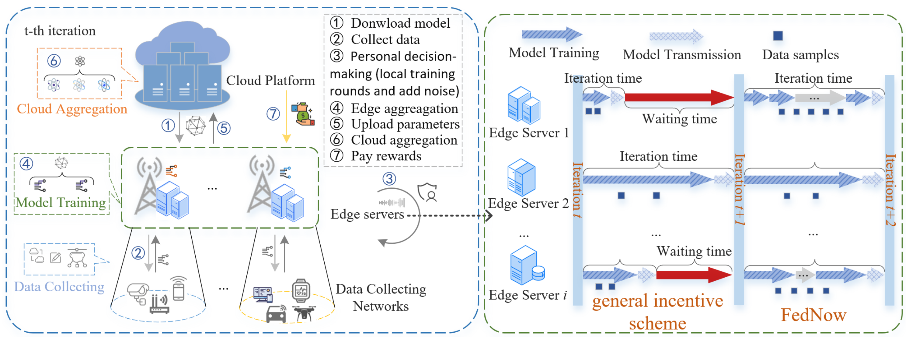
When deriving the optimal rewards for each type of edge server, most of the existing works tend to prioritize incentivizing low-cost edge servers [20,30,41]. However, they often overlook the importance of resource efficiency, i.e., when the low-cost edge servers are providing more data for local model training, some expensive but computationally powerful edge servers may have already completed the local training, resulting in significant waiting times and resource waste for the entire participating group. In contrast, if the platform tends to choose the edge servers with the strongest computing ability, it may lead to excessive payment costs and, thus, low profits. In order to solve this dilemma, we expect to achieve a better trade-off between economic incentives and training efficiency.

4.2. Efficiency Score Function Design

Before presenting our efficiency score function, we first calculate the total costs of the general incentive mechanism that does not consider multiple rounds of local training, and we take this as the upper-bound cost of our optimization scheme. Hence, we obtain

Theorem 1. 

For any solution, from $(s_j^{\prime },{\mathcal{J}}^{\prime })$ to $\left({\mathbb{P}}_2\right)$, it is a feasible solution if and only if the platform’s costs under such a solution are lower than the upper-bound cost, $\overline{U_S}$, i.e.,

$$\begin{array}{cc}\hfill U_S^{\prime }(s_j^{\prime },{\mathcal{J}}^{\prime })& <\overline{U_S}=\frac{1}{\sqrt{{\sum }_{j\in \mathcal{J}}\frac{1}{{\left(2\xi c_j\right)}^{\frac{2}{3}}}}}+\xi \left|\mathcal{J}\right|\sum _{j\in \mathcal{J}}\frac{c_j}{{\left(2\xi c_j\right)}^{\frac{2}{3}}}\hfill \\ \hfill & +\xi \sum _{j=1}^{\mathcal{J}-1}{I}_j·\sum _{i=j+1}^{\mathcal{J}}\left(c_i-c_{i-1}\right)\frac{1}{I_i{\left(2\xi c_i\right)}^{\frac{2}{3}}}.\hfill \end{array}$$

(10)

Proof. 

See Appendix C. □

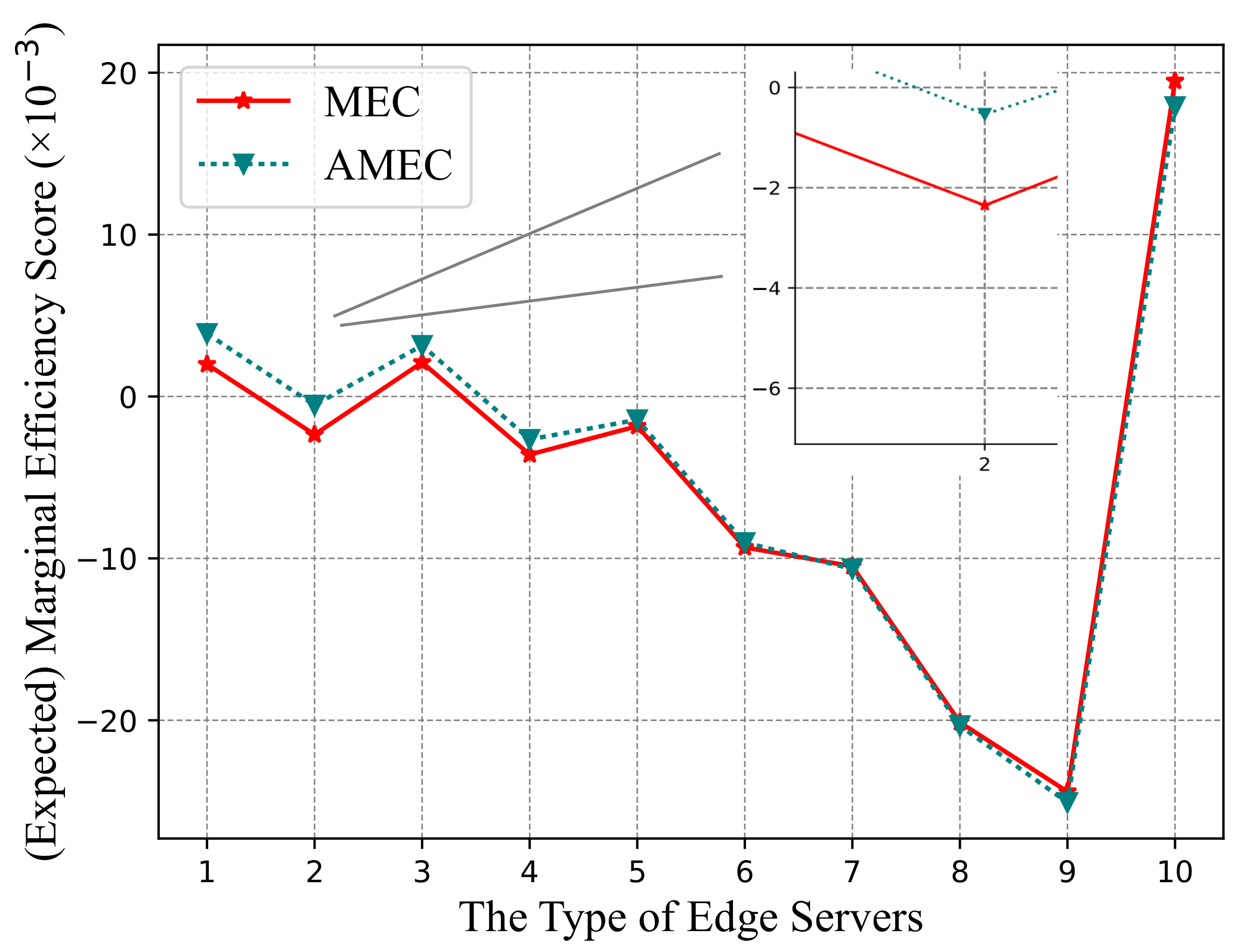
After deriving the upper-bound cost of problem $\left({\mathbb{P}}_2\right)$ (Theorem 1), a general method that can be used is to relax integer constraints and then obtain a feasible solution that satisfies the constraints by rounding, but it cannot guarantee both the existence and the quality of the feasible solutions. Inspired by [25,42], we consider $\left({\mathbb{P}}_2\right)$ as a high-efficiency participant selection problem, which aims to select an appropriate number of edge servers with the best score to form the incentivized set. We consider the edge servers that can generate higher benefits (i.e., lower model accuracy loss) at lower costs as high-efficiency participants and define marginal efficiency costs (MECs) as our efficiency score function, expressed as follows:

$$\begin{array}{cc}\hfill & e_j=U_S\left(\mathcal{J}\right)-U_S(\mathcal{J}/\left\{j\right\})\hfill \\ \hfill & =\frac{1}{\sqrt{{\sum }_{j\in \mathcal{J}}{r}_j{I}_j{s}_j}}+\xi \sum _{j\in \mathcal{J}}{r}_j{I}_j{p}_j-\frac{1}{\sqrt{{\sum }_{j\in \mathcal{J}/\left\{j\right\}}{r}_j{I}_j{s}_j}}-\xi \sum _{j\in \mathcal{J}/\left\{j\right\}}{r}_j{I}_j{p}_j^{\prime },\hfill \end{array}$$

(11)

where $p_j^{\prime }$ denotes the optimal rewards for type set $\mathcal{J}/\left\{j\right\}$ (since the number of types changes, the optimal rewards that decrease (by type) will also change accordingly). Given $s_j$, it is evident that the MECs are influenced by the local training rounds $r_j$. However, the edge servers’ CPU-cycle frequency f is private information and unobservable by the platform. In order to calculate the efficiency score of the edge servers without access to their private attributes, we introduce an exponential mechanism [33], defined as follows:

Definition 3 

(Exponential mechanism). There exists a random mechanism ${\mathcal{M}}_e$ and a score function $q(r,v)$, where $r\to \mathcal{R}$ is the input and $v\to \mathcal{V}$ is the output of the mechanism; ${\mathcal{M}}_e$ satisfies ϵ-differential privacy if

$$\begin{array}{c}\hfill \mathrm{Pr}\left[{\mathcal{M}}_e\left(r\right)=v\right]\propto \exp \left(\frac{ϵq(r,v)}{2\Delta q}\right),\end{array}$$

(12)

where $\Delta q$ is the global sensitivity of the score function, which is defined as the maximum distance between any two input scores, i.e., $\Delta q=\max |q(r,v)-q(r^{*},v)|$.

The definition of the exponential mechanism indicates that each edge server has a probability, $P\left(r_j^{\prime }\right|r_j)$, to determine its local training round as $r_j^{\prime }$. Moreover, the closer $r_j^{\prime }$ and $r_j$ are, the greater the probability $P\left(r_j^{\prime }\right|r_j)$ is. As a result, $q(r_j,r_j^{\prime })$ can be defined as

$$\begin{array}{c}\hfill q(r_j,r_j^{\prime })=-{|r_j-r_j^{\prime }|}^{\frac{1}{2}}.\end{array}$$

(13)

Thus, the global sensitivity $\Delta q=\max |q-q^{\prime }|={(r_{max}-r_{min})}^{\frac{1}{2}}={(\overline{\theta }-1)}^{\frac{1}{2}}$. For any local training round $r_j\in \mathcal{R}=\{1,2,\cdots ,\overline{\theta }\}$, the platform can calculate the mapping probability $P\left(r_j^{\prime }\right|r_j)$ as

$$\begin{array}{c}\hfill P\left(r_j^{\prime }\right|r_j)=\frac{exp\left(ϵ\frac{-{|r_j-r_j^{\prime }|}^{\frac{1}{2}}}{2\Delta q^{\frac{1}{2}}}\right)}{{\sum }_{r^{*}\in \mathcal{R}}exp\left(ϵ\frac{-{|r_j-r^{*}|}^{\frac{1}{2}}}{2\Delta q^{\frac{1}{2}}}\right)}.\end{array}$$

(14)

For the mapping probability $P\left(r_j^{\prime }\right|r_j)$, the platform can use the expected rounds, $\mathbb{E}\left(r_j\right)$, to approximate the edge servers’ true local training rounds $r_j$, i.e., given $P\left(r_j^{\prime }\right|r_j)$, $r^{\prime }\in \mathcal{R}$, the expected local training rounds can be calculated by

$$\begin{array}{c}\hfill \mathbb{E}\left(r_j\right)=\sum _{r^{\prime }\in \mathcal{R}}{r}_j^{\prime }P\left(r_j^{\prime }\right|r_j)=\sum _{r^{\prime }\in \mathcal{R}}{r}_j^{\prime }\frac{exp\left(ϵ\frac{-{|r_j-r_j^{\prime }|}^{\frac{1}{2}}}{2\Delta q^{\frac{1}{2}}}\right)}{{\sum }_{r_j^{*}\in \mathcal{R}}exp\left(ϵ\frac{-{|r_j-r_j^{*}|}^{\frac{1}{2}}}{2\Delta q^{\frac{1}{2}}}\right)}.\end{array}$$

(15)

Therefore, the approximate marginal efficiency cost (AMEC) can be expressed as

$$\begin{array}{cc}\hfill & {\tilde{e}}_j=\frac{1}{\sqrt{{\sum }_{j\in \mathcal{J}}\mathbb{E}\left(r_j\right)I_j{s}_j}}+\xi \sum _{j\in \mathcal{J}}\mathbb{E}\left(r_j\right)I_j{p}_j-\hfill \\ \hfill & \frac{1}{\sqrt{{\sum }_{j\in \mathcal{J}/\left\{j\right\}}\mathbb{E}\left(r_j\right)I_j{s}_j}}-\xi \sum _{j\in \mathcal{J}/\left\{j\right\}}\mathbb{E}\left(r_j\right)I_j{p}_j^{\prime }.\hfill \end{array}$$

(16)

The platform sorts each type of edge server according to their AMEC in ascending order. A smaller AMEC indicates a higher margin utility and higher quality. The platform will select edge servers according to their AMEC from low to high until finding a threshold type, $x^{\prime }$, such that $U_S\left({\mathcal{J}}^{\prime }\right)\le \overline{U_S}$ and $U_S({\mathcal{J}}^{\prime }\cup \left\{{\overline{e}}_{x^{\prime }+1}\right\})>\overline{U_S}$, where ${\mathcal{J}}^{\prime }$ represents the set of selected edge servers (Assuming there are only five types of edge servers: {1, 2, 3, 4, and 5} and $x^{\prime }=4$. Since the order sorted by the edge servers’ AMEC may not follow the same order as their contract types, e.g., AMEC: {2, 1, 4, 3, and 5}, then ${\overline{e}}_{x^{\prime }}\triangleq 3$, ${\overline{e}}_{x^{\prime }+1}\triangleq 5$, and $({\overline{e}}_{x^{\prime }}+1)\triangleq 4$). For the selected set ${\mathcal{J}}^{\prime }$, we denote $J^{\prime }=\left|{\mathcal{J}}^{\prime }\right|$ and re-index the edge servers’ type in ${\mathcal{J}}^{\prime }$ by ${\left\{j\right\}}_{j\in \{1,\cdots ,J^{\prime }\}}$ in ascending order of training cost, $c_j$. However, since the platform’s cost, $U_S$, is affected by both $r_j$ and $s_j$, even if the incentivized set ${\mathcal{J}}^{\prime }$ is determined, the platform may be able to obtain a better feasible solution by adjusting its data requirements $s_j,\forall j\in {\mathcal{J}}^{\prime }$. Based on the above analysis, we obtain

Proposition 1. 

Given a set of contract items ${\varphi }_j=(p_j,s_j)$ and $\overline{\theta }$, where $\forall j\in \mathcal{J},$

(i) 

if ${\sum }_{j\in {\mathcal{J}}^{\prime }}{r}_j{I}_j{s}_j>{\sum }_{j\in \mathcal{J}}{I}_j{s}_j$ and ${\sum }_{j\in {\mathcal{J}}^{\prime }}{r}_j{I}_j{p}_j^{\prime }<{\sum }_{j\in \mathcal{J}}{I}_j{p}_j$, there exists a threshold type $x^{\prime }$, such that $U_S^{\prime }(s_j,{\mathcal{J}}^{\prime })<\overline{U_S}$, where

$$\begin{array}{c}\hfill p_j^{\prime }=\left\{\begin{array}{c}{c}_j{s}_j,\mathrm{if}j=J^{\prime },\hfill \\ c_j{s}_j+\sum _{i=j+1}^{J^{\prime }}\left(c_i-c_{i-1}\right)s_i,\hfill \\ \mathrm{if}j\ne J^{\prime }\mathrm{and}j=\{1,\cdots ,\left(J^{\prime }-1\right)\}.\hfill \end{array}\right.\end{array}$$

(ii) 

if the threshold type $x^{\prime }$ exists, there exists an optimal type $x^{*}$ and required data size $s_j^{*}$ such that $U_S^{*}(s_j^{*},{\mathcal{J}}^{*})\le U_S^{\prime }(s_j,{\mathcal{J}}^{\prime })$, where ${\mathcal{J}}^{*}$ is the platform’s optimal incentivized type set.

Proof. 

See Appendix D. □

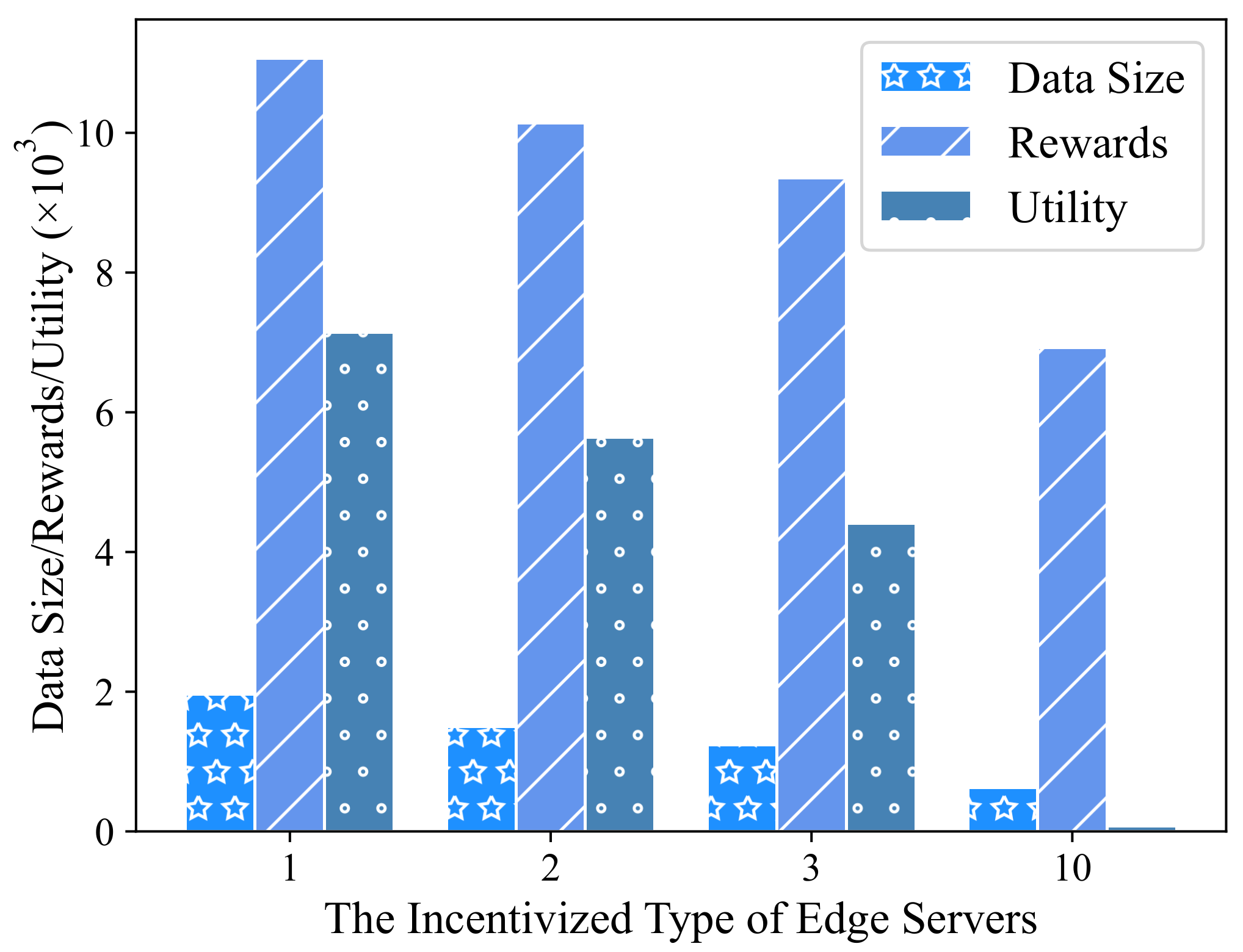
Proposition 1(i) shows that, given $s_j$, the optimal choice for the platform is to incentivize the edge servers that can provide more total data at lower payment costs. In addition, the platform only provides positive contract items for the incentivized type of edge servers, whereas the non-incentivized edge servers will receive zero contract items. Proposition 1(ii) suggests that if a feasible solution exists, the platform can adjust its incentive strategy (i.e., required data size $s_j$), which may lead to a better solution that minimizes the platform’s costs. According to the above analysis, we first designed an iterative algorithm to determine all incentivized edge servers and then characterized the training process of FedNow, which enables the edge servers to personally determine their local training rounds; we used the Monte Carlo method to obtain a better (near-optimal) response for the platform, including the incentivized set ${\mathcal{J}}^{*}$ and corresponding ${\{s_j^{*},p_j^{*}\}}_{j\in {\mathcal{J}}^{*}}$. With ${\mathcal{J}}^{*}$ and ${\{s_j^{*},p_j^{*}\}}_{j\in {\mathcal{J}}^{*}}$, the incentivized edge servers will honestly complete model training to compute the optimal global model parameters.

The details of searching for feasible solutions are shown in Algorithm 1. The platform first calculates all edge servers’ AMEC (Line 2–4), then sorts the edge servers based on their AMEC in ascending order and searches for the threshold type $x^{\prime }$ (Line 5–18). The time complexity of calculating ${\tilde{e}}_j$ (Line 4) is $O\left(\mathcal{J}\right)$, while the time complexity for checking whether the feasibility condition holds (Line 11) is also $O\left(\mathcal{J}\right)$. Therefore, the time complexity of Algorithm 1 is $\mathit{O}\left({\mathcal{J}}^2\right)$.

Algorithm 1 Calculation of the feasible solution $(x^{\prime },{\mathcal{J}}^{\prime })$

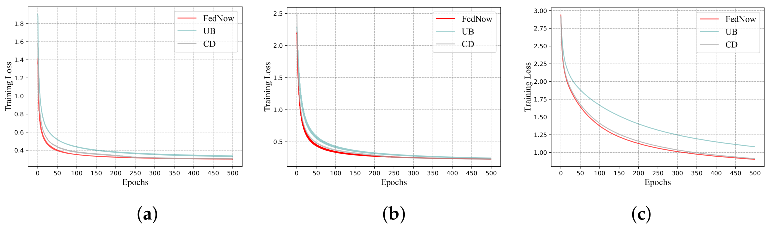
Algorithm 2 describes the training process of FedNow when computing the optimal model parameters. The time complexity of the Monte Carlo method is $\mathit{O}\left(N\right)$, where N means the number of sampling times. For a strongly convex objective $F\left(\omega \right)$, the general upper bound of global iterations is expressed as $T_{\mathrm{ite}}(\kappa ,\zeta )=\frac{\mathit{O}(log(1/\sigma \left)\right)}{1-\zeta }$ [43], which is affected by both global accuracy $\kappa$ and local accuracy $\zeta$. Given a fixed global accuracy $\sigma$, the upper bound of the local iterations, i.e., $\mathit{O}(log(1/\sigma \left)\right)$, can be normalized to 1 so that $T_{\mathrm{ite}}\left(\zeta \right)=\frac{1}{1-\zeta }$ [16]. We represent the time used for one global iteration of FEL as $T_{\mathrm{glob}}\left(\xi \right)$; the upper bound of the time complexity for Algorithm 2 is $\mathit{O}\left(max\{N,\frac{1}{1-\xi }·T_{glob}\left(\zeta \right)\}\right)$.

Algorithm 2 The training process of FedNow

5. Experiments

In this section, we first exhibit the experimental setup and then show the experiments conducted on both the synthetic and real datasets to evaluate the performance of our proposed FedNow.

5.1. Experimental Setup

Edge server parameters. By referring to [7,37], we considered a cloud platform, a set of $\left|\mathcal{I}\right|=100$ edge servers for FEL. We leveraged two GPU devices (i.e., Lenovo Notebooks with NVIDIA RTX 3060 and NVIDIA GTX 1050Ti, Beijing, China) with multi-thread programming to simulate the training process of heterogeneous edge servers. For simplicity, the platform divides edge servers into several groups based on their training costs, c, and CPU frequency, f, and we approximate each group as a supertype [30]. By limiting computing resources to a range from 0.8 GHz to 2.7 GHz, we divided the edge servers into 10 groups, where the edge servers with $(c_j,f_j)$ uniformly distributed over $\left(\right[1.5,2.4]$×$[0.8,0.9])$∪$\left(\right[2.5,3.4]$×$[1.0,1.1])$∪$\left(\right[3.5,4.4]$×$[1.2,1.3])$∪$\left(\right[4.5,5.4]$×$[1.4,1.5])$∪$\left(\right[5.5,6.4]$×$[1.6,1.7])$∪$\left(\right[6.5,7.4]$×$[1.8,1.9])$∪$\left(\right[7.5,8.4]$×$[2.0,2.1])$∪$\left(\right[8.5,9.4]$×$[2.2,2.3])$∪$\left(\right[9.5,10.4]$×$[2.4,2.5])$∪$\left(\right[10.5,11.4]$×$[2.6,2.7])$. We took the midpoint of each group to represent the cost and CPU frequency of their supertype, e.g., approximately $(c_j,f_j)=(2.3,0.8)\approx (2.0,0.85)$ as the type-1 edge server (According to [30], approximating edge server type with reagrd to several supertypes will not significantly affect the platform’s payment and utility.).

Training parameters. We constructed an FL model using MLP, CNN, and ResNet-18, respectively, and trained them by exploiting benchmark datasets: MNIST, Fashion MNIST, and CIFAR-10. The MLP network is formed by two convolutional layers with a max-pooling of 2, fully connected layers, a Relu activation function, and a softmax output layer, whereas the CNN model has two convolutional layers with a kernel size of 5, two dense layers, and a softmax output layer. The ResNet-18 model is made up of a feedfoward layer, a fully connected layer (size = 1000), and a softmax output layer, where the feedforward layer includes four convolutional layers and eight residual blocks. We set the economic conversion parameter to $\xi =9\times {10}^{-8}$ and the learning rate to 0.01.

Baselines. In order to demonstrate the performance of FedNow, we adopted two state-of-the-art solutions as the baselines, described as follows:

• UB: A vanilla contract incentive mechanism that assumes each edge server only conducts one round of local training (Theorem 1). We consider that it represents the upper-bound cost of any feasible strategy.
• CD: A cost-driven incentive mechanism that considers the multi-local training rounds of edge servers but prefers to motivate low-cost edge servers [20,30]. We compared it with FedNow to demonstrate the effectiveness of the efficiency score function.

Metrics. For the synthetic dataset, we used model accuracy loss: $acc.l=\frac{1}{\sqrt{{\sum }_{j\in \mathcal{J}}{r}_j{I}_j{s}_j}}$, payment costs: $P={\sum }_{j\in \mathcal{J}}{r}_j{I}_j{p}_j$, and the platform’s total costs: $U_S=acc.l+\xi P$ to assess the performance of FedNow in terms of economic incentives. In the real datasets, we used (i) model accuracy and accuracy loss, (ii) average waiting time, (iii) training efficiency, and (iv) completion time, respectively, to evaluate the performance of FedNow. Concretely, we recorded the changes in model accuracy over time and accuracy loss with epoch under different strategies. Moreover, for the different strategies, we recorded the average waiting time of all edge servers in each epoch. Based on this, we could calculate the overall average waiting time $\overline{\mathcal{W}}$ and the overall average epoch time $\overline{\mathcal{V}}$ for different strategies, thus deriving their training efficiency (defined as $1-\overline{\mathcal{W}}/\overline{\mathcal{V}}$ [4]). $\overline{\mathcal{W}}$ and $\overline{\mathcal{V}}$ are represented as follows:

$$\begin{array}{c}\hfill \left\{\begin{array}{c}\overline{\mathcal{W}}=\frac{1}{T}\sum _{t=1}^T{\mathcal{W}}^t,\hfill \\ \overline{\mathcal{V}}=\frac{1}{T}\sum _{t=1}^T{\rho }^t.\hfill \end{array}\right.\end{array}$$

where ${\mathcal{W}}^t$ means the overall average waiting time of the edge servers in epoch t, and ${\rho }^t$ denotes the time spent on completing the t-th epoch, which can be measured by recording the training time of the slowest edge server at the t-th epoch (${\rho }^t\le t_a,\forall t\in \{1,\cdots ,T\}$). Moreover, we also recorded the completion time of Fednow and the two baselines when achieving the same training accuracy.

5.2. Evaluation of the Synthetic Dataset

For the first set of experiments, we used to verify the superiority and rationality of our mechanism in terms of economic utility. Concretely, we first demonstrated how FedNow selects more efficient edge servers, and we verified the rationality of the incentive design. Then, we performed experiments on the synthetic dataset to evaluate the performance of the different strategies.

Figure 2 shows the MECs and AMECs of different types of edge servers. Apparently, the MECs and AMECs of the type-1, -3, and -10 edge servers were both greater than 0, which means that the cost contribution of the type-1, -3, and -10 edge servers is positive, considering that the smaller the MEC/AMEC (i.e., smaller cost increment), the higher the value/efficiency of the corresponding edge servers. In contrast, the MEC and AMEC of the type-2, -4–9 edge servers are both less than 0, which means that they have negative effects on the platform’s costs. In other words, when MEC/AMEC is less than zero, the smaller the MEC/AMEC, the lower the priority of selecting the corresponding type of edge server. In addition, since the training cost of type-10 edge servers is the largest, then, when calculating the efficiency score of the other types of edge servers, the type-10 edge servers are always in the incentivized set ${\mathcal{J}}^{\prime }$, and the platform’s optimal payment for them will just cover their training costs, making the type-10 edge servers always a critical payment type. When calculating the efficiency score of the type-10 edge servers, the critical payment type changes from 10 to 9, which may lead to a significant reduction in server payment costs. The above two factors explain the intense changes in efficiency scores between the type-9 and type-10 edge servers. Therefore, when the platform has complete information about the local training rounds of the edge servers, the preference order is $\{1,3,10,5,2,4,6,7,8,9\}$, whereas the preference order under incomplete information is $\{3,1,10,2,5,4,6,7,8,9\}$.

Table 2. Differences in performance for different metric; LR means the local training rounds, and D denotes the overall data size contributed by the incentivized set ${\mathcal{J}}^{\prime }$.

Ref.	${\mathcal{J}}^{\prime }$	LR	D$(\times {10}^3)$	acc.l$(\times {10}^{-2})$	P$(\times {10}^4)$	${\mathit{U}}_{\mathit{S}}$$(\times {10}^{-1})$
UB	{1, ⋯, 10}	1	10.3583	0.3107	9.2625	0.1152
Control Group	{1, 2, 3}	$r_j,j\in {\mathcal{J}}^{\prime }$	2.4602	0.6375	6.5252	0.1231
CD	{1, 2, 3, 4, 5}	$r_j,j\in {\mathcal{J}}^{\prime }$	7.5857	0.363	7.5447	0.1048
MEC	{1, 3, 5, 10}	$r_j,j\in {\mathcal{J}}^{\prime }$	10.4166	0.3098	7.0024	0.0946
FedNow	{1, 2, 3, 10}	$r_j,j\in {\mathcal{J}}^{\prime }$	9.0836	0.3317	7.4569	0.1009

characterizes the performance differences of different strategies under their respective optimal incentive solutions. According to the control group, it is clear that the lack of data size leads to a significant accuracy loss, thus making the total costs higher than UB, even if the payment costs are the lowest. The cost-driven incentive strategy (CD) could incentivize more types of edge servers to participate, but this also leads to higher payment costs, whereas when reducing the incentivized types, the decrease in data size causes an increase in accuracy loss and may make the total cost $U_S$ higher than UB. Moreover, in Table 2, we denote MEC as the efficiency-aware incentive mechanism with complete information about edge servers’ local training rounds. Obviously, with the complete information about $r_j$, MEC achieves the best performance on both accuracy loss and payment costs, thereby minimizing the total costs of the platform. Due to the influence of incomplete information, although the preference order and the optimal incentivized set of FedNow are different from MEC, FedNow can achieve similar performance to MEC and outperform the cost-driven strategy.

Figure 3 shows that the platform provides positive contract items for the incentivized type of edge servers, and the critical type of edge servers (i.e., type-10 edge servers) only obtain 0 utility since the optimal rewards provided to type-10 edge servers by the platform just cover their training costs.

5.3. Evaluation Using the Real Datasets

The second set of experiments evaluated the training performance of our mechanism according to accuracy and loss when using the real datasets. We first used training loss to evaluate the performance of the three strategies. Figure 4 shows the training loss of three strategies trained with different datasets over the epochs. As training progresses, the training loss of FedNow and the two baselines both decrease with epoch, but the loss curve of FedNow clearly has the fastest decline and a faster convergence rate than the baselines. For example, in Figure 4a, when the epoch approaches 50, FedNow begins to converge, and its loss is below 0.4, while the training loss for the baselines is obviously higher than 0.4; it takes CD and UB an additional 50 and 100 epochs, respectively, to achieve a similar loss. Second, considering the fact that different strategies may have different training times in each epoch, we recorded the variation in training accuracy over time, as shown in Figure 5. Due to the ease of training with MNIST and FMNIST, the three strategies ultimately achieve similar training accuracies, as seen in Figure 5a,b; in contrast, CD achieves the highest training accuracy in Figure 5c, which may due to the fact that tending toward low-cost edge servers can motivate relatively more training samples with the same budgets. However, it is worth noting that since FedNow prioritizes selecting more efficient edge servers and allows them to personally decide their local training rounds (i.e., multiple local training rounds), the model trained with FedNow can converge over a time that is obviously shorter. For example, in FMNIST and CIFAR-10, the model trained with FedNow converges nearly 100 and 300 s earlier than CD, respectively. Moreover, CD allows multiple local training rounds but tends to choose low-cost edge servers, which leads to more training samples but also longer training times. UB requires each edge server to perform only one round of local training, which makes the overall training time under this strategy relatively short. However, this also leads to insufficient training samples/local training rounds for UB, resulting in the slowest convergence speed and the worst model accuracy. In Figure 6, in order to demonstrate the effectiveness of the efficiency-aware mechanism, we further intuitively represent the completion time when the model trained using the three strategies reaches the same accuracy. Excitingly, the completion time of FedNow is the lowest among the three training strategies. For instance, in Figure 6c, it takes 393 s, 681 s, and 801 s for a model to obtain the training accuracy of 0.75 when trained with FedNow, CD, and UB, respectively. In other words, for CIFAR10-ResNet18, FedNow saves more training time than CD and UB by as much as 42.3% and 51% when reaching an accuracy of 0.75.

Based on the above results, we found that enabling personal decision-making during local training rounds could ensure satisfactory convergence speed and shorten completion time when reaching the same training accuracy. Therefore, even in a situation where resources are limited (e.g., the limited payment budgets), FedNow can improve model convergence speed and achieve a better final model accuracy than those solutions that only consider payment costs or ignore edge server personal decision-making.

The third set of experiments was performed to evaluate the training efficiency of the different strategies. Figure 7 characterizes the average waiting time for the different strategies with epochs. Figure 7 indicates that the average waiting time for the three strategies remains relatively stable, and Fednow’s performance in resource utilization is still the best. For example, for MNIST-MLP in Figure 7a and FMNIST in Figure 7b, the average waiting time for the two baselines is around 0.125 s and 0.15 s, respectively, whereas that of FedNow is 0.05 s and 0.75 s, which indicates that FedNow reduces the average waiting time by at least 50% when compared to the baseline method. Moreover, the average waiting time of CD is only slightly lower than that of UB, which indicates that a preference for low-cost edge servers cannot effectively solve the problem of low training efficiency. Last but not least, we present the training efficiency and testing accuracy of the three strategies in

Table 3. Training efficiency and test accuracy of three strategies

	MNIST-MLP		FMNIST-CNN		CIFAR10-RESNET
	Efficiency	Test_acc	Efficiency	Test_acc	Efficiency	Test_acc
UB	0.4109	0.9546	0.4132	0.9800	0.4787	0.7874
CD	0.6672	0.9667	0.6780	0.9822	0.7010	0.8435
FedNow	0.8247	0.9833	0.8027	0.9838	0.8357	0.8332

.

Based on the above results, we found that FedNow could improve resource utilization and reduce useless waiting times. This is because the performance gaps between heterogeneous devices are narrowed by allowing for different local training rounds and data requests. Hence, comprehensively considering an edge server’s personal decision-making and individual efficiency can alleviate the negative effect of a synchronization barrier for those edge devices with heterogeneous computation capacities.

6. Conclusions

In this work, we propose a novel, efficiency-aware incentive mechanism, FedNow, that can motivate data contribution and efficient resource utilization without accessing edge servers’ private attributes. On the basis of contract incentive boundaries, we have carefully designed an efficiency score function to prioritize more efficient edge servers. Subsequently, we have derived sufficient conditions for making FedNow outperform existing schemes in terms of joint optimization objectives. Extensive simulations on both synthetic and real datasets show that our efficiency-aware incentive mechanism can improve training efficiency and resource utilization by at least 15.53% and 22.78%, respectively.

In future research, we consider that this work can be extended/deepened in multiple directions and mention two ideas as examples. First, when compared to the solution that requires edge servers to maintain the same local update frequency, allowing multiple rounds of local training can narrow the performance gap between heterogeneous edge servers, which, to some extent, enhances the fairness of the FEL system. As far as we know, although there have been some efforts made to focus on controlling client participation frequency to achieve better fairness [44], few of these introduce the axiomatized fairness concept or rigorously derive optimal solutions based on maximizing social fairness. Therefore, improving training efficiency while strictly ensuring social fairness remains an open topic that, although challenging, is of great significance for promoting the sustainable co-operation of clients in FEL. Second, in this work, to resist privacy breaches that may be caused by an untrusted platform, we introduced an exponential mechanism and designed FedNow to motivate clients’ contributions without accessing their private attributes and true training strategies. In future work, we expect to generalize our work to situations where both the platform and clients are untrusted while still incentivizing efficient co-operation between honest clients and the platform. The explanations of mathematical terms used in all formulas are shown in

Table 4. Expand Table 1: An explanation of the mathematical terms used in the formulas.

Mathematical Terms	Physical Meanings
$f_d\left(\omega \right)$, $F_j\left(\omega \right)$, $\omega$, ${\omega }^{*}$	The prediction loss on a pair of data samples d, the loss function of edge server j, the model parameter, and the optimal model parameters.
$c_i^t$, $c_i^p$, $c_i^l$, $c_i^m$	The total costs of edge server i in t-th global epoch; the unit computation cost, unit data-collection cost, and unit communication cost of edge server i.
$S_d$, $I_j$	The global model size (fixed), and the number of edge servers contained in the type set j.
$T_j^p$, $\tau$, $f_j$	The computation time for a type-j edge server to perform one local training round, the number of CPU cycles required for performing one sample of data, and the CPU-cycle frequency of a type-j edge server.
$U_j(c_j,{\varphi }_j,r_j)$, $u_j(c_j,{\varphi }_j)$	The total utilities of type-j edge servers; the unit-round utility of type-j edge servers, equivalent to the utility of completing contract per time.
$\xi$, $s_j^{*}$, $p_j^{*}$	The platform’s weight regarding the rewards and the optimal data size/rewards for type-j edge servers.
$U_S$, $\overline{U_S}$	The utility function of the platform, equivalent to the platform’s total costs; the cost upper-bound of the platform.
$\Delta q$	The global sensitivity of the score function.
$r_j$, $r_j^{\prime }$, $\mathcal{R}$	The real training rounds of type-j edge servers, the expected training rounds of type-j edge servers, the set of possible training rounds.
$U_S\left(\mathcal{J}\right)$, $U_S(\mathcal{J}/\left\{j\right\})$	The total costs of the platform when the incentivizing set is $\mathcal{J}$ and $\mathcal{J}/\left\{j\right\}$, respectively.
$T_{\mathrm{ite}}(\kappa ,\zeta )$	The general upper bound of global iterations; $\kappa$: global accuracy, $\zeta$: local accuracy.
${\mathcal{W}}^t$, $\overline{\mathcal{W}}$	Waiting time in the t-th epoch and the overall average waiting time.
${\mathcal{V}}^t$, $\overline{\mathcal{V}}$, ${\rho }^t$	Epoch time in the t-th epoch, the overall average epoch time, and the training time of the slowest edge server in the t-th epoch.

.