Article

Automatic GNSS Ionospheric Scintillation Detection with Radio Occultation Data Using Machine Learning Algorithm

1
China Research Institute of Radiowave Propagation, Qingdao 266107, China
2
National Key Laboratory of Electromagnetic Environment, Qingdao 266107, China
3
School of Electronic Engineering, Xidian University, Xi’an 710071, China
*
Author to whom correspondence should be addressed.
Appl. Sci. 2024, 14(1), 97; https://doi.org/10.3390/app14010097
Submission received: 13 November 2023 / Revised: 5 December 2023 / Accepted: 7 December 2023 / Published: 21 December 2023
(This article belongs to the Special Issue Intelligent Computing and Remote Sensing)

Abstract

:
Ionospheric scintillation often occurs in the polar and equator regions, and it can affect the signals of the Global Navigation Satellite System (GNSS). Therefore, the ionospheric scintillation detection applied to the polar and equator regions is of vital importance for improving the performance of satellite navigation. GNSS radio occultation is a remote sensing technique that primarily utilizes GNSS signals to study the Earth’s atmosphere, but its measurement results are susceptible to the effects of ionospheric scintillation. In this study, we propose an ionospheric scintillation detection algorithm based on the Sparrow-Search-Algorithm-optimized Extreme Gradient Boosting model (SSA-XGBoost), which uses power spectral densities of the raw signal intensities from GNSS occultation data as input features to train the algorithm model. To assess the performance of the proposed algorithm, we compare it with other machine learning algorithms such as XGBoost and a Support Vector Machine (SVM) using historical ionospheric scintillation data. The results show that the SSA-XGBoost method performs much better compared to the SVM and XGBoost models, with an overall accuracy of 97.8% in classifying scintillation events and a miss detection rate of only 12.9% for scintillation events with an unbalanced GNSS RO dataset. This paper can provide valuable insights for designing more robust GNSS receivers.

1. Introduction

In recent years, the widespread use of GNSS PNT services [1] has made it increasingly important to enhance the security and reliability of global satellite navigation systems. The ionosphere serves as a crucial pathway for the transmission of satellite carrier signals, forming a link between the near-Earth atmosphere and outer space. The potential threat it poses to the GNSS PNT service is widely recognized. Investigations into ionospheric scintillation hold vital importance in enhancing the reliability of GNSS PNT services.
The ionosphere is an atmospheric layer located approximately 60~1000 km above the Earth’s surface. The ionosphere is the most exceptional layer of the Earth as it is the most outer one towards outer space. Therefore, the ionosphere can contain important information. As it was discovered by Victor Hess around 1912 [2], the whole of the Earth’s atmosphere has played a historical role in the discovery and in the progress of ubiquitous cosmic radiation. The ionosphere consists of atmospheric molecules that are made up of ions and electrons with non-uniformly varying densities, resulting in structural inhomogeneity. When the GNSS carrier signal travels through the irregular ionosphere structure [3], it experiences rapid fluctuations in its time delay, amplitude, and phase. This is known as scintillation [3], which is caused by various factors, including solar activity, magnetic storms, local electric fields, and wave interactions, among others factors [4,5]. Scintillation can affect the amplitude and phase of the GNSS carrier signal to different extents. This can result in the deterioration of positioning accuracy and continuity performance. Ionospheric scintillation is broadly classified into two types: amplitude scintillation and phase scintillation. Amplitude scintillation results in the rapid disruption of the signal carrier-to-noise ratio, a reduction in the quality of the signal-to-noise ratio, and the halting of signal transmission via satellite [6]. Alternatively, phase scintillation can result in weekly fluctuations in the carrier phase, which could have detrimental effects such as signal loss in severe cases [7,8]. Many vital civil and military installations are dependent on GNSS systems. Therefore, the creation of effective techniques for identifying ionospheric scintillation has become exceedingly crucial for ionospheric investigation and for improving the precision of GNSS devices.
There are numerous factors that influence the intensity of ionospheric scintillation, and among them, geographical location is one of the critical factors. In the case of L-band satellite signals, ionospheric scintillation is notably most severe in the polar and equator regions [9,10]. Data indicate that satellite communication near the polar and equator regions can be unreliable, with receivers often unable to capture the transmitted signal, resulting in interrupted navigation [11]. Additionally, there is a seasonal trend in the variation in ionospheric scintillation [12] throughout the year, with a higher frequency of occurrences during the spring and autumn equinoxes. The scintillation is particularly intense during the spring equinox.
Current research into ionospheric scintillation detection relies heavily on ground-based ionospheric scintillation monitoring (ISM) stations [13,14]. While these stations offer prolonged and continuous monitoring, their limited geographic coverage means they are unable to capture the diverse range of scintillation features present in different regions. Additionally, the cost of deploying a sufficient number of ground-based ISM stations globally is prohibitively expensive. GNSS radio occultation (RO) [15] is an objective remote sensing approach. It involves receiving electromagnetic wave signals emitted by high-orbiting GNSS satellites and measuring them in the L1 (1575.42 MHz) and L2 (1227.42 MHz) frequency bands via GNSS receivers installed on LEO satellites. When GNSS carrier signals pass through the ionosphere, the radio wave path bends. With the movement of satellites at both the signal transmitting and receiving ends, the signal path sweeps through the atmosphere for a few tens of seconds to minutes, either from high to low or from low to high. This phenomenon is known as an occultation event, and measurements of it may be sensitive to ionosphere effects. The geometry of GNSS RO is displayed in Figure 1. GNSS RO operates globally, covering all geographical regions. It presents the opportunity to detect and record diverse scintillations geographically and builds on existing LEO satellites to reduce the cost of large-scale system monitoring.
GNSS RO measurements currently play a significant role in the observation of ionospheric space weather [16,17]. RO observations from the FengYun-3C (FY3C) satellite during the St. Patrick’s Day geomagnetic storm in 2015 demonstrated a significantly altered likelihood of ionospheric scintillation events [18]. The incidence of scintillation was found to have increased in the New Zealand region during the main phase of the storm, as determined by the TEC gradient. Conversely, during the recovery phase after the geomagnetic storm, the incidence of scintillation was reduced.
Previous research has primarily focused on detecting changes in satellite signal amplitude and phase caused by ionospheric scintillation. This involves computing the amplitude scintillation index ( S 4 ) and the phase scintillation index ( σ φ ) and using dedicated ionospheric scintillation monitoring receivers [19] that are programmed with predetermined thresholds for the S 4 and σ φ indices to detect ionospheric scintillation events [20]. However, the utilization of this thresholding technique necessitates complex filtering and detrending operations on the observations. It neglects the high-dimensional feature information of the GNSS signals [21]. Moreover, the conventional thresholding techniques are highly susceptible to false alarms stimulated by multipaths and cannot determine precise thresholds under varying conditions, leading to poor detection accuracy for weak scintillation events. Wavelet transformation techniques [22] have been proposed as a replacement to detrending operations. However, said techniques rely on intricate implementations. In recent times, researchers have explored different machine learning methods for detecting ionospheric scintillation. Jiao et al. utilized Support Vector Machines (SVMs) to detect ionospheric amplitude and phase scintillations [23,24], which involved the incorporation of a significant amount of authentic scintillation data during the training phase. As a result, they attained a detection accuracy of 91–96%, surpassing conventional thresholding techniques. However, Support Vector Machine (SVM) classifiers require significant memory allocations for sizable datasets, which incurs high computational expenses. Furthermore, the overfitting issue persists, thereby leading to misleading outcomes. Linty et al. have introduced a decision tree (DT)-based algorithm for detecting ionospheric scintillation [25], utilizing in-phase and orthogonal values from the receiver tracking loop output as sample features. The algorithm can achieve a detection accuracy of 98%, with a very low false alarm rate. However, obtaining in-phase and quadrature correlator output values is challenging and requires a specific receiver.
In this study, an ionospheric scintillation detection model is developed utilizing the Sparrow Search Algorithm (SSA)-optimized XGBoost. The GNSS radio occultation technique is used to compute the power spectral density (PSD) of the GNSS signal strength by extracting the signal strength during an occultation event, which is then employed as a training feature in the detection model to achieve ionospheric scintillation detection and subsequently apply it to global regions, especially the polar and equator regions. A thorough comparison with established SVM and XGBoost algorithms demonstrates that the ionospheric scintillation detection model presented in this study outperforms them. The Sparrow Search Algorithm, with its robust global optimization capabilities, is employed to optimize some of the hyperparameters in XGBoost. These refinements enhance the model’s performance and operational efficiency, reducing the likelihood of overfitting in the detection classification task. The innovative aspect of this study lies in the utilization of an optimized XGBoost algorithm for ionospheric scintillation detection (which is subsequently applied to global regions, especially the polar and equator regions), as well as its quantitative analysis and comparison of machine learning algorithm performance with regard to accuracy, precision, recall, and F-Score.
The remainder of this paper is structured as follows: Section 2 provides a detailed description of the XGBoost model, as well as an overview of the Sparrow Search Algorithm and how it can optimize XGBoost. Section 3 outlines the development of the GNSS RO dataset for the detection of ionospheric scintillations and presents the experimental procedure and corresponding evaluation criteria used for our quantitative analysis of the results. Finally, the results obtained are scrutinized, and different machine learning algorithms are compared. Section 4 summarizes the findings and provides a prospective outlook on future studies.

2. SSA-XGBoost Model

2.1. XGBoost

The XGBoost algorithm [26], introduced by Tianqi Chen in 2016, enhances the robustness of a learning algorithm through gradient boosting. This entails iteratively reducing the loss function along the gradient direction. Additionally, integrated learning involves merging multiple weak classifiers into a stronger one via a certain combinatorial strategy. Doing so improves the efficiency and accuracy of classification. XGBoost can fully utilize multi-core CPUs for parallel computation [26], thereby diminishing running time. Compared to other extensively applied machine learning algorithms, such as Support Vector Machines [27], XGBoost offers several benefits. It operates with higher efficiency and classification accuracy and is also highly scalable and sparse-aware, rendering it optimal for handling datasets with irregular and imbalanced training data. Ionospheric scintillation is influenced by different factors, and the resulting imbalance between scintillating and non-scintillating data presents a challenge, but XGBoost can effectively address this by establishing the direction of gradient descent [28].
XGBoost consists of a number of different decision trees [29], each of which corresponds to a new function f i ( x ) , and the core of which is to continuously learn a new function f i ( x ) to fit the residuals of the prediction of the previous function f i 1 ( x ) , i.e., it will keep adding decision trees and keep splitting the features during the computation process [26]. After completing the training process and obtaining K decision trees, the model needs to predict new data. For a given training dataset S = { ( x i ,   y i ) } ,   ( | S | = n ,   x i R m ,   y i R ) with n samples and m features, y i is the labelled value of the training samples, and for the binary classification task, y i ∈ (0, 1). The predicted outputs y i of the model after having K decision trees are as follows:
y ˆ i = k = 1 K f k x i ,   f k F
where F = f ( x ) = ω q ( x ) q : R m T , ω R is the space of the decision trees, the tree structure q and the leaf weights ω represent the two parts that make up a decision tree, and T denotes the number of leaf nodes in the tree.
According to the characteristics of the samples, f k x maps these samples to the corresponding leaf nodes in each tree and assigns a score, and the sum of the scores of each tree is used as the predicted value of the sample. Obviously, the ultimate goal of the XGBoost algorithm is to make the predicted values of all trees as close as possible to the corresponding true values [26] with the strongest generalization ability. On top of the current tree, another tree is added to fit the residuals between the predicted values of the previous tree and the corresponding true values. In order to select the next added tree, an objective function [26] is introduced, which combines a loss function and a rule function, and it is by minimizing this objective function that the integrated learning of XGBoost is achieved, as shown below:
O b j ( k ) = i = 1 n l y i , y ˆ i ( k 1 ) + f k x i + Ω f k
where i denotes the ith sample, n is the number of samples, y i is the true score of the current tree, y ˆ i ( k 1 ) denotes the predicted value of the k 1 tree, and l is a loss function that measures the distance between y i and y ˆ i ( k 1 ) . f k is the new function of the current tree, and Ω f k is the corresponding regularization term to keep the overall model complexity within the desired range and avoid overfitting, thus producing a more accurate model.
XGBoost approximates the above objective function using the second-order Taylor series to derive a new objective function as follows:
O b j ( k ) = i = 1 n l y i , y ˆ i ( k 1 ) + g i f k x i + 1 2 h i f k 2 x i + Ω f k = i = 1 n g i ω q x i + 1 2 h i ω q 2 x i + γ T + λ 1 2 j = 1 T h i ω j 2
where g i = y ˆ ( t 1 ) l y i ,   y ˆ ( t 1 ) , h i = 2 y ˆ ( t 1 ) l y i , y ˆ ( t 1 ) , ω j is the weight of the jth leaf node, and γ and λ are used to control the complexity of the tree. G j = i I j g i and H j = i I j h i are the optimal leaf weights:
ω j * = G j H j + λ
Then, the optimal objective function for a given tree structure q can be obtained as follows:
O b j ( k ) = j = 1 T G j ω j + 1 2 H j ω j 2 + γ T = 1 2 j = 1 T G j H j + λ + γ T
Then, the greedy algorithm is employed to enumerate all possible tree structures q to identify the optimal splitting node of the leaf node and attain the maximum gain of the objective function following the split [26]; this greedy algorithm starts from a single leaf node and iteratively adds branches to the tree, assuming that I L and I R are the sets of instances of left and right sub-trees of the node, respectively, so that I = I L I R . Then, the gain after the splitting of the leaf node j is expressed as follows:
G a i n = 1 2 G L 2 H L + λ + G R 2 H R + λ G L + G R 2 H L + H R + λ γ
where G L and G R are the first-order gradient values of the left and right leaf nodes after splitting; H L and H R are the corresponding second-order gradient values. The first, second, and third terms of the formula correspond to the scores of the left leaf node, the right leaf node, and the observed leaf node, respectively, and γ serves as a regularization parameter to prevent the over-splitting of the decision tree.
Figure 2 shows a brief schematic of the XGBoost algorithm.
The XGBoost algorithm controls the construction of the tree by setting some hyperparameters to limit the complexity and weight of each tree [26]. Table 1 shows several important hyperparameters of the XGBoost algorithm, which have different degrees of influence on the performance of the XGBoost algorithm.
Each hyperparameter has a different range of values, resulting in a large number of combinations. The traditional method of finding the optimal hyperparameters is to set a certain range for each hyperparameter based on experience and then perform a grid search within that range, calculate the accuracy of each combination, and select the combination with the highest accuracy, which is a set of optimal hyperparameters. The traditional method is easy to understand and implement, but the disadvantages include the fact that it relies on personal experience, the fact that the grid search calculation is relatively large and time-consuming, and the fact that it is easy to fall into the local optimal solution, leading to the model classification effect, which is difficult to optimize. To address the above problems, this study uses the Sparrow Search Algorithm to find the optimal hyperparameters of XGBoost.

2.2. Sparrow Search Algorithm

The Sparrow Search Algorithm (SSA) [30] is a novel swarm intelligence optimization algorithm that was proposed by Jiankai Xue et al. in 2020 and based on the foraging process of sparrows. A colony of sparrows is composed of three sparrow types: discoverers, joiners, and warners. These types continuously update their positions during foraging to locate the best food source. The optimal food source position represents the most favorable solution.
The following assumptions are made:
(1)
When a sky enemy approaches a sparrow colony and is detected, the colony shifts position in time;
(2)
Under certain circumstances, the identities of the discoverers and the joiners are interchangeable;
(3)
The lower the fitness value of an individual sparrow, the harsher and more dangerous the area in which it forages.
Based on the above assumptions, the SSA model is constructed as shown below, with X representing the current position of the sparrow population, expressed in the form of a matrix:
X = x 1,1 x 1,2 x 1 , d x 2,1 x 2,2 x 2 , d x n , 1 x n , 2 x n , d
where n is the number of sparrows, and d is the number of parameters to be optimized. In the SSA, fitness values are used to assess the foraging ability of individual sparrows, and the matrix of fitness values for the entire sparrow population is shown below:
F X = f ( [ x 1,1 x 1,2 x 1 , d ] ) f ( [ x 2,1 x 2,2 x 2 , d ] ) f ( [ x n , 1 x n , 2 x n , d ] )
Here, f x i , 1 x i , 2 x i , d is used to calculate the fitness value of the ith sparrow at the current location.
Discoverers have high fitness values in the sparrow flock. They are more capable of foraging and can provide the group with the location and direction of foraging. During each iteration, the location of the discoverer is updated with the following rules:
X i , j t + 1 = X i , j t exp i α i t e r m a x   if   R 2 < S T X i , j t + Q L   if   R 2 S T
where t is the number of iterations; X i , j t denotes the location information of the ith sparrow in the jth dimension; α ( α ∈ [0, 1]) is a random number; i t e r m a x is the maximum number of iterations; Q is a random stone obeying a normal distribution; L is a 1 × d matrix, where each element in L i is either −1 or 1; R 2 ( R 2 ∈ [0, 1]) denotes the discoverer’s optimal individual fitness value at t time; and S T S T 0.5 , 1 denotes the safety value. When R 2 < S T , it means that there is no natural enemy around the foraging environment at this time, and the discoverer conducts an extensive grid search to find the location of the locally optimal fitness value; when R 2 > S T , it indicates that there is a natural enemy around the foraging environment at this time and that the sparrow colony needs to go to a new safe location to forage.
There are two types of joiners in a sparrow colony: the first are those with high fitness values, which are mainly responsible for monitoring the discoverer, and as soon as they know that the finder has found a better foraging location, they will immediately fly to the vicinity of the discoverer to compete with him; the second are those with low fitness values, which forage elsewhere to increase the fitness value in order to wait for the time when it is suitable to compete with the discoverer, and the position updating rule of the joiners is as follows:
X i , j t + 1 = Q exp X worst   X i , j t i 2   if   i < n 2 X p t + 1 + X i , j t X P t + 1 A + L   otherwise  
where X p is the optimal location for the current discoverer to forage; X w o r s t is the current most unfavorable location; and A is a 1 × d matrix, where each element of the matrix is randomly assigned to be either −1 or 1, A + = A T A A T 1 , when i > n 2 joiners with lower adaptation values do not obtain food and must move to other locations to forage.
Some of the individuals in the joiner group are randomly selected to be early warners, and the rules for updating the location of early warners are as follows:
X i , j t + 1 = X b e s t t + β X i , j t X b e s t t   if   f i > f g X i , j t + K X i , j t X w o r s t t f i f w + ε   if   f i = f g
where X b e s t is the position of the discoverer that finds the best foraging position at the current moment; X w o r s t is the position of the discoverer that finds the worst foraging position for food; K denotes the current fitness value of the sparrow; β represents the direction of movement of the sparrow, which is a random number; f g is the value of the global optimal fitness; f w is the value of the global worst fitness; and ε is used to ensure that the denominator is not 0. When f i > f g , it means that the sparrow is at the edge of the group and is very vulnerable to attack by natural enemies; when f i = f g , it means that the sparrow in the middle of the group is aware of the danger and needs to be close to the other sparrows in order to minimize the risk of being attacked by natural enemies.

2.3. Optimize XGBoost Using the Sparrow Search Algorithm

Optimizing some hyperparameters in XGBoost through using the Sparrow Search Algorithm, with its strong global optimization capability, can improve the classification performance and operational efficiency of the model, and the steps of optimization are as follows:
Step 1: initialize the Sparrow-Search-Algorithm-related parameters and XGBoost-related parameters.
Step 2: the mean absolute error obtained through cross-validation is utilized as a function of individual sparrow fitness values, with the retention of the best fitness values and positional internalization.
Step 3: calculate the warning value, and based on its magnitude, update the discoverer’s position following the discoverer update position rule.
Step 4: update the position of the joiner based on the joiner update position rule.
Step 5: update the position of the sparrows that perceive danger based on the early warner update position rule, where the sparrows at the edge of the population move closer to the safe area and the sparrows at the center of the population move randomly to get closer to the other sparrows.
Step 6: to update the global optimal information, calculate the sparrow’s updated individual fitness value and compare it to the original fitness value.
Step 7: Determine if the number of iterations satisfies the termination condition. If not, repeat step 2. If it does, stop and output the optimum parameters.
Figure 3 illustrates the final SSA-XGBoost model structure.

3. Experiments

This section firstly establishes the GNSS RO dataset, secondly describes the overall flow of the experiment, and finally presents the evaluation criteria for the quantitative analysis of the results, discussing the classification performance of the designed model on the basis of different metrics.

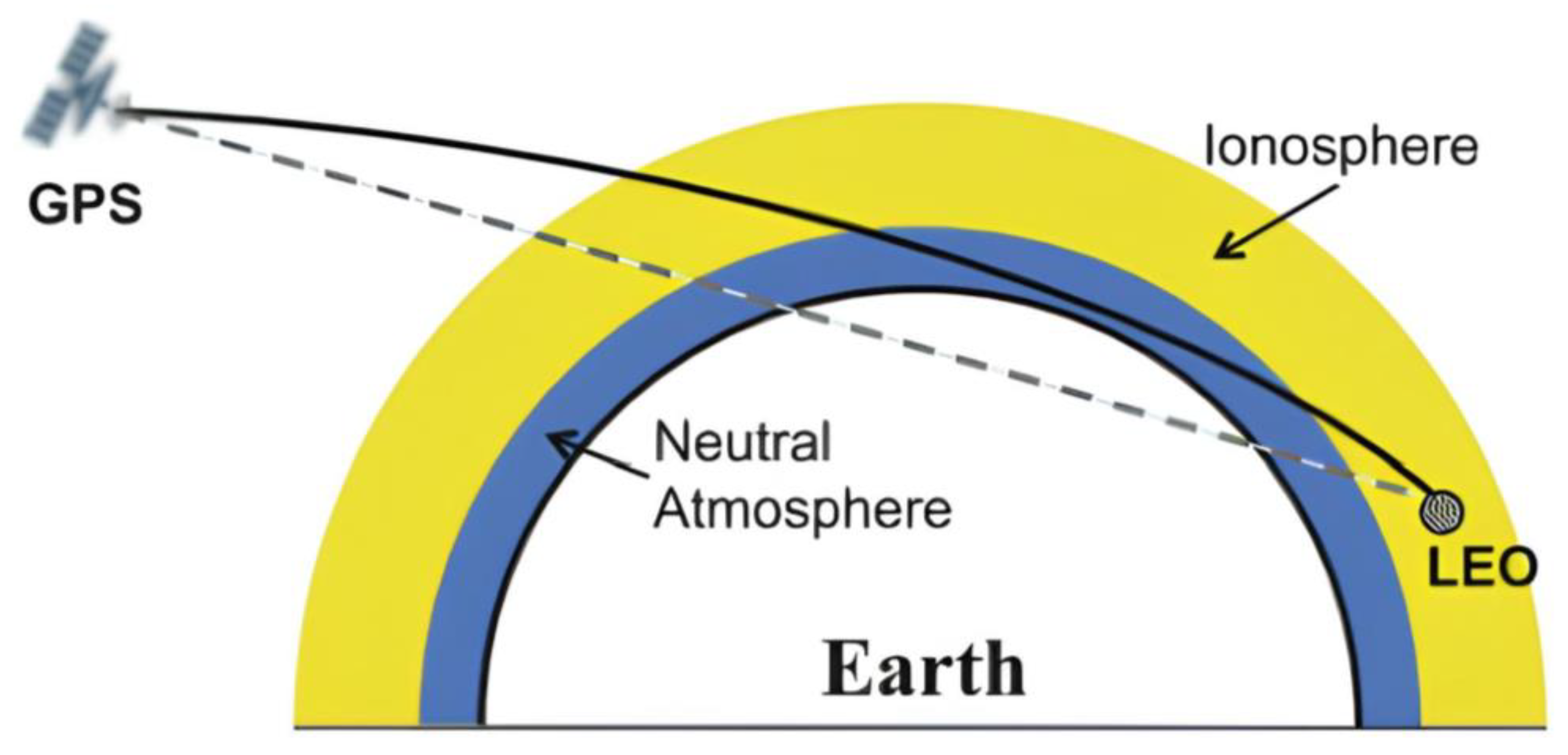
3.1. GNSS RO Dataset

Scintillation in the polar and equator regions strongly affects the phase and amplitude of GNSS carrier signals [31]. In this study, some measurements recorded using the MetOp-A occultation [32] between 2015 and 2018 are used. The navigation receiver on MetOp-A can receive GPS L1 C/A code signals [33] and is capable of outputting raw satellite signal strengths sampled at 50 H z , and Figure 4 shows some examples of satellite signal strength variations from MetOp-A occultation measurements.
The signal strength of a satellite may be utilized to compute the power spectral density of the satellite signal. This PSD [34] is the Fourier transform of the autocorrelation function of the signal strength and can be evaluated through using the Welch method [35,36] (modified periodogram averaging method). The Welch method computation steps are as follows:
(a)
The signal with data length N is divided equally into L segments, each with data length M;
(b)
The selected window function is added to each small segment of data, and the periodogram for each segment is derived to form a modified periodogram, which is then averaged over each modified periodogram;
(c)
Each corrected periodogram is approximated as uncorrelated with each other, and the result (processed using a smoothing algorithm) is used as the final power spectral density map.
In particular, this study uses occultation events for which scintillation has been recorded [37], and these occultation events are labelled by setting label 1 for scintillation events and label 0 for non-scintillation events. The average duration of an occultation event is 22 s, which means that the power spectral density of the satellite signal is computed within an average time window of 22 s and is input into the classification model as a data sample along with the labelled values of the corresponding occultation events. Table 2 provides an overview of the detailed structure of this dataset, with the first column being the class labels and the second to last column being the PSD computed using the Welch method, with each row constituting a row vector entered into the model as a data sample.

3.2. Experimental Procedure

The overall flow of the experiment includes the processing of the MetOp-A occultation measurement data, extracting the feature covariates of interest, tagging the data samples, and finally producing a dataset; 75% of the produced dataset is used as a training set to train the model, and 25% is used as a test set to validate the model’s performance [38], and the designed ionospheric magnitude based on the SSA-XGBoost algorithm scintillation detection model was compared with machine learning algorithms such as XGBoost and Support Vector Machines using the same dataset, as shown in Figure 5.

3.3. Evaluation Criteria

The performance of the model was evaluated by the confusion matrix [39], accuracy, precision, recall, and F-score [40]. The confusion matrix shows information about the correct classification and misclassification of the test data. Figure 6 shows an example of the confusion matrix; it has four quadrants, and here are what they mean: True Negative (TN) is an outcome where the model correctly predicts the negative class; False Positive (FP) is an outcome where the model incorrectly predicts the positive class; False Negative (FN) is an outcome where the model incorrectly predicts the negative class; True Positive (TP) is an outcome where the model correctly predicts the positive class; the larger the percentage of TN and TP, the higher the classification accuracy of the model.
Based on the results of the confusion matrix, the corresponding accuracy, precision, recall, and F-score can be calculated as follows:
A c c u r a c y = T N + T P T N + F P + F N + T P       P r e c i s i o n = T P T P + F P R e c a l l = T P T P + F N F-score = 2   Precision     Recall     Precision   +   Recall  
where accuracy represents the number of correct classifications made by the model as a proportion of all data, precision represents the accuracy of the model in judging potential events as occurring blinks, and recall refers to the percentage of correctly predicted classifications labelled 1 as a proportion of the true categories. Precision and recall are sometimes contradictory, and they are considered together using the F-score [35], which is taken as a weighted average of them, with a higher F-score indicating a more effective classification model.

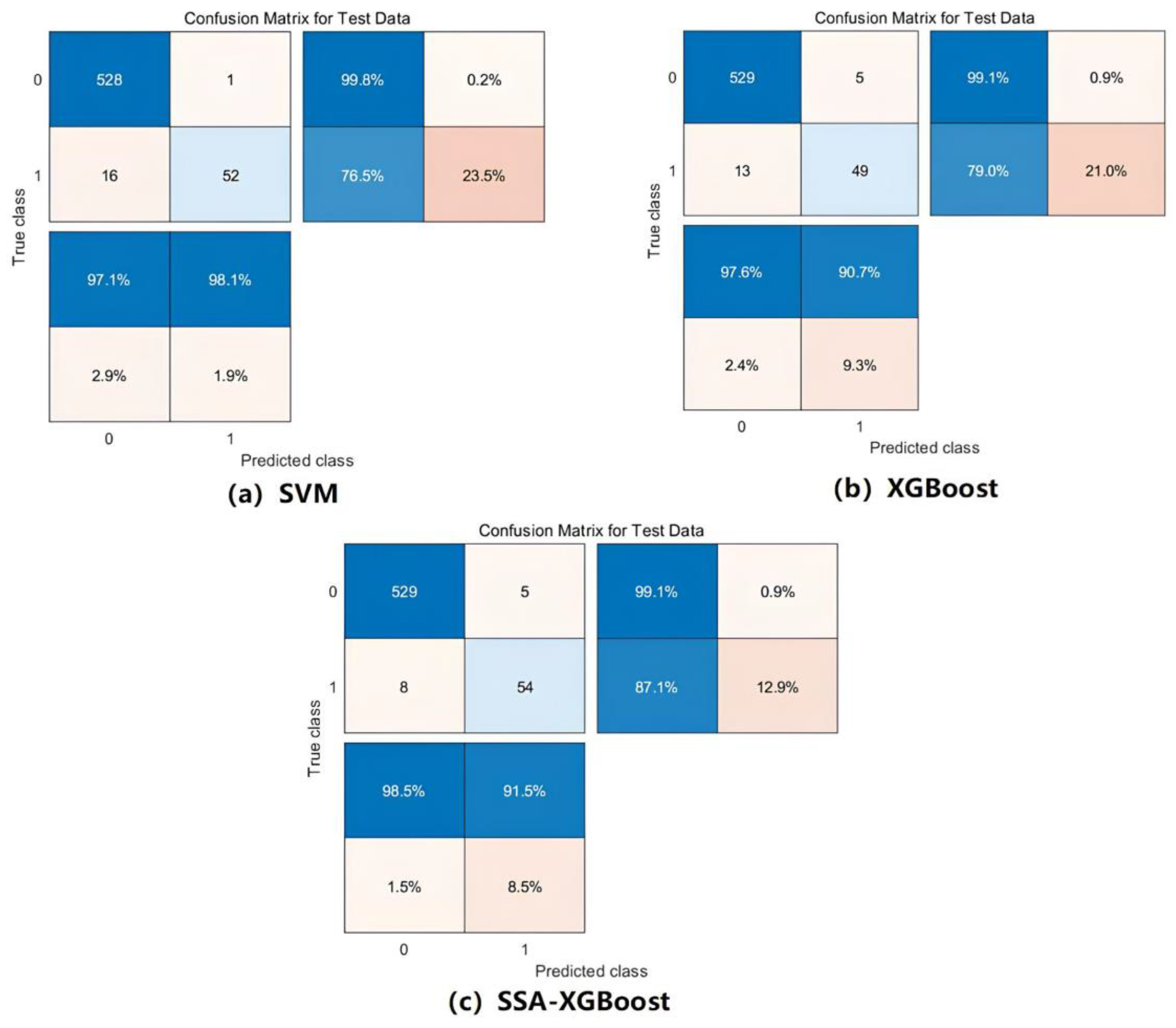
3.4. Results and Analysis

This study involved evaluating the performance of an ionospheric scintillation detection model that used the SSA-XGBoost algorithm. This model was compared to SVM and XGBoost algorithms on a test set. The resulting confusion matrices for the SSA-XGBoost, SVM, and XGBoost algorithms are shown in Figure 7, along with accuracy rates of 97.1% (SVM), 96.9% (XGBoost), and 97.8% (SSA-XGBoost), demonstrating that the SSA-XGBoost model, in the context of detecting and classifying ionospheric scintillation, provides superior performance compared to the SVM and XGBoost models.
The leakage rates of the SVM and XGBoost models for the flicker events are 23.5% and 21%, respectively, while the leakage rate of the SSA-XGBoost model for the flicker events is only 12.9%, which suggests that the detection model can more accurately capture the features of the flicker events after optimizing XGBoost using the Sparrow Search Algorithm.
More detailed evaluation metrics are shown in Table 3. The F-score of the SSA-XGBoost-based ionospheric scintillation detection model proposed in this study is 89.2%, which is even better compared to that of the SVM and XGBoost models, indicating that the detection model proposed in this study is more effective. It is worth noting that the performance of the detection model varies with each execution of the model since 75% of the training set is randomly selected from the entire dataset.

4. Conclusions

In this study, we developed a model (the Sparrow-Search-Algorithm-optimized XGBoost model) to detect ionospheric scintillation and subsequently applied it to global regions, applying it to the polar and equator regions in particular. This involved analyzing GNSS RO measurements obtained from the MetOp-A satellite between 2015 and 2018. Our findings are consistent with similar studies employing data from ground-based ionospheric scintillation monitoring stations [23].
The power spectral density of the GNSS signal is used as input in the ionospheric scintillation detection model, unlike other conventional methods like computation of amplitude and phase scintillation indices [41], and the power spectral density does not require a complicated detrending procedure. Rather, it only necessitates a fast Fourier transform (FFT) module [42], which can be obtained more easily. This benefit facilitates the integration of the ionospheric scintillation detection method using GNSS signal power spectral density as a detection characteristic into LEO satellites, which holds immense importance in building space-based ionospheric scintillation monitoring networks [43].
The algorithm proposed in this study underwent evaluation to ascertain its test set performance. The classification achieved an overall accuracy of 97.1542%, with just a 12.9% miss detection rate for scintillation occasions. This performance was higher than that of the SVM and XGBoost models. It is shown that the model proposed in this study is of great value for the detection of ionospheric scintillation in the polar and equator regions.
This study involved solely detecting ionospheric scintillation in GNSS RO measurements from the MetOp-A satellite. In future research, RO measurements from various LEO satellite constellations in diverse geographic locations will be collected to expand on the characteristics of scintillation.

Author Contributions

Conceptualization, G.J., R.J. and W.Z.; methodology, G.J. and R.J.; analysis, G.J.; validation, G.J.; discussion, G.J., R.J. and H.Y.; writing—original draft preparation, G.J.; writing—review and editing, R.J. All authors took part in the discussion of the work described in this paper. All authors have read and agreed to the published version of the manuscript.

Funding

The National Natural Science Foundation of China (No. 52371354).

Institutional Review Board Statement

Not applicable.

Informed Consent Statement

Not applicable.

Data Availability Statement

Code and data can be provided by the authors upon request.

Acknowledgments

The authors wish to extend their gratitude to the research teams specializing in ionospheric scintillation detection, and the authors would like to thank the University Corporation for Atmospheric Research/COSMIC Data Analysis and Archive Center (UCAR/CDAAC) for sharing the MetOp-A RO data, which were used in this work.

Conflicts of Interest

The authors declare no conflict of interest.

References

  1. Zuo, Z.Y.; Qiao, X.; Wu, Y.B. Concepts of comprehensive PNT and related key technologies. In Proceedings of the 2019 International Conference on Modeling, Analysis, Simulation Technologies and Applications (MASTA 2019), Hangzhou, China, 26–27 May 2019; Atlantis Press: Amsterdam, The Netherlands, 2019; pp. 365–370. [Google Scholar]
  2. Hess, V.F. Über Beobachtungen der durchdringenden Strahlung bei sieben Freiballonfahrten. Z. Phys. 1912, 13, 1084. [Google Scholar]
  3. Jiang, C.; Wei, L.; Yang, G.; Aa, E.; Lan, T.; Liu, T.; Zhao, Z. Large-scale ionospheric irregularities detected by ionosonde and GNSS receiver network. IEEE Geosci. Remote Sens. Lett. 2020, 18, 940–943. [Google Scholar] [CrossRef]
  4. Jiao, Y. Low-Latitude Ionospheric Scintillation Signal Simulation, Characterization, and Detection on GPS Signals. Ph.D. Thesis, Colorado State University, Fort Collins, CO, USA, 2017. [Google Scholar]
  5. Li, Q.; Yin, P. The characteristic study of ionospheric scintillations over China based on GNSS data. In Proceedings of the Ninth Annual China Satellite Navigation Symposium-S01 Satellite Navigation Application Technology 2018, Harbin, China, 23–25 May 2018; pp. 190–195. [Google Scholar]
  6. De Oliveira Moraes, A.; da Silveira Rodrigues, F.; Perrella, W.J.; de Paula, E.R. Analysis of the characteristics of low-latitude GPS amplitude scintillation measured during solar maximum conditions and implications for receiver performance. Surv. Geophys. 2012, 33, 1107–1131. [Google Scholar] [CrossRef]
  7. Linty, N.; Minetto, A.; Dovis, F.; Spogli, L. Effects of phase scintillation on the GNSS positioning error during the September 2017 storm at Svalbard. Space Weather 2018, 16, 1317–1329. [Google Scholar] [CrossRef]
  8. Xu, B.; Liu, D. Ionospheric Scintillation Effects on GNSS. GNSS World China 2011, 36, 5–8. [Google Scholar]
  9. An, P.; Xiao, Z.; Tang, X.; Sun, G. The Effect of Ionospheric Scintillation on Receiver. GNSS World China 2017, 42, 47–54. [Google Scholar]
  10. Liu, D.; Fen, J.; Deng, Z.; Zhen, W. Analysis of Ionospheric Scintillation Effects on GNSS Positioning. GNSS World China 2009, 34, 1–8. [Google Scholar]
  11. Pan, L.; Yin, P. Analysis of polar ionospheric scintillation characteristics based on GPS data. In Proceedings of the China Satellite Navigation Conference (CSNC) 2014 Proceedings: Volume I, Nanjing, China, 21–23 May 2014; Springer: Berlin/Heidelberg, Germany, 2014; pp. 11–18. [Google Scholar]
  12. Ahmed, W.A.; Wu, F.; Agbaje, G.I.; Ednofri, E.; Marlia, D.; Zhao, Y. Seasonal ionospheric scintillation analysis during increasing solar activity at mid-latitude. In Optics in Atmospheric Propagation and Adaptive Systems XX; SPIE: Bellingham, WA, USA, 2017; Volume 10425, pp. 66–78. [Google Scholar]
  13. Yu, X.; Yue, X.; Zhen, W.; Xu, J.; Liu, D.; Guo, S. On the occurrence of F region irregularities over Haikou retrieved from COSMIC GPS radio occultation and ground-based ionospheric scintillation monitor observations. Radio Sci. 2017, 52, 34–48. [Google Scholar] [CrossRef]
  14. Liu, Y.; Fu, L.; Wang, J.; Zhang, C. Study of GNSS loss of lock characteristics under ionosphere scintillation with GNSS data at Weipa (Australia) during solar maximum phase. Sensors 2017, 17, 2205. [Google Scholar] [CrossRef]
  15. Bonafoni, S.; Biondi, R.; Brenot, H.; Anthes, R. Radio occultation and ground-based GNSS products for observing, understanding and predicting extreme events: A review. Atmos. Res. 2019, 230, 104624. [Google Scholar] [CrossRef]
  16. Yue, X.; Schreiner, W.S.; Pedatella, N.; Anthes, R.A.; Mannucci, A.J.; Straus, P.R.; Liu, J.Y. Space weather observations by GNSS radio occultation: From FORMOSAT-3/COSMIC to FORMOSAT-7/COSMIC-2. Int. J. Res. Appl. 2014, 12, 616–621. [Google Scholar] [CrossRef]
  17. Liu, J.Y.; Lin, C.H.; Rajesh, P.K.; Lin, C.Y.; Chang, F.Y.; Lee, I.T.; Chen, S.P. Advances in ionospheric space weather by using FORMOSAT-7/COSMIC-2 GNSS radio occultations. Atmosphere 2022, 13, 858. [Google Scholar] [CrossRef]
  18. Wang, G.; Shi, J.; Bai, W.; Galkin, I.; Wang, Z.; Sun, Y. Global ionospheric scintillations revealed by GPS radio occultation data with FY3C satellite before midnight during the March 2015 storm. Adv. Space Res. 2019, 63, 3119–3130. [Google Scholar] [CrossRef]
  19. Vankadara, R.K.; Jamjareegulgarn, P.; Seemala, G.K.; Siddiqui, M.I.H.; Panda, S.K. Trailing Equatorial Plasma Bubble Occurrences at a Low-Latitude Location through Multi-GNSS Slant TEC Depletions during the Strong Geomagnetic Storms in the Ascending Phase of the 25th Solar Cycle. Remote Sens. 2023, 15, 4944. [Google Scholar] [CrossRef]
  20. Taylor, S.; Morton, Y.; Jiao, Y.; Triplett, J.; Pelgrum, W. An improved ionosphere scintillation event detection and automatic trigger for GNSS data collection systems. In Proceedings of the 2012 International Technical Meeting of The Institute of Navigation, Nashville, TN, USA, 17–21 September 2012; pp. 1563–1569. [Google Scholar]
  21. Su, K.; Jin, S.; Hoque, M.M. Evaluation of ionospheric delay effects on multi-GNSS positioning performance. Remote Sens. 2019, 11, 171. [Google Scholar] [CrossRef]
  22. Mushini, S.C.; Jayachandran, P.T.; Langley, R.B.; MacDougall, J.W.; Pokhotelov, D. Improved amplitude-and phase-scintillation indices derived from wavelet detrended high-latitude GPS data. GPS Solut. 2012, 16, 363–373. [Google Scholar] [CrossRef]
  23. Jiao, Y.; Hall, J.J.; Morton, Y.T. Automatic equatorial GPS amplitude scintillation detection using a machine learning algorithm. IEEE Trans. Aerosp. Electron. Syst. 2017, 53, 405–418. [Google Scholar] [CrossRef]
  24. Jiao, Y.; Hall, J.; Morton, Y.J. Automatic GPS phase scintillation detector using a machine learning algorithm. In Proceedings of the 2017 International Technical Meeting of The Institute of Navigation 2017, Monterey, CA, USA, 2–30 January 2017; pp. 1160–1172. [Google Scholar]
  25. Linty, N.; Farasin, A.; Favenza, A.; Dovis, F. Detection of GNSS ionospheric scintillations based on machine learning decision tree. IEEE Trans. Aerosp. Electron. Syst. 2018, 55, 303–317. [Google Scholar] [CrossRef]
  26. Chen, T.; Guestrin, C. Xgboost: A scalable tree boosting system. In Proceedings of the 22nd ACM SIGKDD International Conference on Knowledge Discovery and Data Mining, San Francisco, CA, USA, 13–17 August 2016; pp. 785–794. [Google Scholar]
  27. Chauhan, V.K.; Dahiya, K.; Sharma, A. Problem formulations and solvers in linear SVM: A review. Artif. Intell. Rev. 2019, 52, 803–855. [Google Scholar] [CrossRef]
  28. Dey, A.; Rahman, M.; Ratnam, D.V.; Sharma, N. Automatic detection of gnss ionospheric scintillation based on extreme gradient boosting technique. IEEE Geosci. Remote Sens. Lett. 2021, 19, 1–5. [Google Scholar] [CrossRef]
  29. Charbuty, B.; Abdulazeez, A. Classification based on decision tree algorithm for machine learning. J. Appl. Sci. Technol. Trends 2021, 2, 20–28. [Google Scholar] [CrossRef]
  30. Xue, J.; Shen, B. A novel swarm intelligence optimization approach: Sparrow search algorithm. Syst. Sci. Control. Eng. 2020, 8, 22–34. [Google Scholar] [CrossRef]
  31. Jiao, Y.; Hall, J.J.; Morton, Y.T. Performance evaluation of an automatic GPS ionospheric phase scintillation detector using a machine-learning algorithm. NAVIGATION J. Inst. Navig. 2017, 64, 391–402. [Google Scholar] [CrossRef]
  32. Bonnedal, M.; Christensen, J.; Carlström, A.; Berg, A. Metop-GRAS in-orbit instrument performance. GPS Solut. 2010, 14, 109–120. [Google Scholar] [CrossRef]
  33. Montenbruck, O.; Andres, Y.; Bock, H.; van Helleputte, T.; van den Ijssel, J.; Loiselet, M.; Yoon, Y. Tracking and orbit determination performance of the GRAS instrument on MetOp-A. GPS Solut. 2008, 12, 289–299. [Google Scholar] [CrossRef]
  34. Youngworth, R.N.; Gallagher, B.B.; Stamper, B.L. An overview of power spectral density (PSD) calculations. Opt. Manuf. Test. VI 2005, 5869, 206–216. [Google Scholar]
  35. Jwo, D.J.; Chang, W.Y.; Wu, I.H. Windowing techniques, the welch method for improvement of power spectrum estimation. Comput. Mater. Contin. 2021, 67, 3983–4003. [Google Scholar] [CrossRef]
  36. Rahi, P.K.; Mehra, R. Analysis of power spectrum estimation using welch method for various window techniques. Int. J. Emerg. Technol. Eng. 2014, 2, 106–109. [Google Scholar]
  37. Ludwig-Barbosa, V.; Sievert, T.; Carlström, A.; Pettersson, M.I.; Vu, V.T.; Rasch, J. Supervised detection of ionospheric scintillation in low-latitude radio occultation measurements. Remote Sens. 2021, 13, 1690. [Google Scholar] [CrossRef]
  38. Guyon, I.; Makhoul, J.; Schwartz, R.; Vapnik, V. What size test set gives good error rate estimates? IEEE Trans. Pattern Anal. Mach. Intell. 1998, 20, 52–64. [Google Scholar] [CrossRef]
  39. Krstinić, D.; Braović, M.; Šerić, L.; Božić-Štulić, D. Multi-label classifier performance evaluation with confusion matrix. Comput. Sci. Inf. Technol. 2020, 1, 1–14. [Google Scholar]
  40. Goutte, C.; Gaussier, E. A probabilistic interpretation of precision, recall and F-score, with implication for evaluation. In Proceedings of the European Conference on Information Retrieval, Santiago de Compostela, Spain, 21–23 March 2005; Springer: Berlin/Heidelberg, Germany, 2005; pp. 345–359. [Google Scholar]
  41. Luo, X.; Gu, S.; Lou, Y.; Cai, L.; Liu, Z. Amplitude scintillation index derived from C/N 0 measurements released by common geodetic GNSS receivers operating at 1 Hz. J. Geod. 2020, 94, 27. [Google Scholar] [CrossRef]
  42. Zhang, D.; Wang, H.; Feng, Y.; Wang, X.; Liu, G.; Han, K.; Chen, J. Fast Fourier transform (FFT) using flash arrays for noise signal processing. IEEE Electron. Device Lett. 2022, 43, 1207–1210. [Google Scholar] [CrossRef]
  43. Sun, H.; Xu, L.; Wang, S.; Wu, Y. Development and Application of Ionospheric Detection Technology. In Proceedings of the 2nd International Conference on Electrical Engineering and Computer Technology (ICEECT 2022), Suzhou, China, 23–25 September 2022; IOP Publishing: Bristol, UK, 2022; Volume 2404, p. 012030. [Google Scholar]
Figure 1. GNSS RO geometry.
Applsci 14 00097 g001
Figure 2. Schematic diagram of the XGBoost algorithm.
Applsci 14 00097 g002
Figure 3. Structure of the SSA-XGBoost model.
Applsci 14 00097 g003
Figure 4. Examples of GPS signal strength fluctuations recorded by the MetOp-A occultation. The left panel shows more dramatic signal strength fluctuations.
Applsci 14 00097 g004
Figure 5. Experimental flow.
Applsci 14 00097 g005
Figure 6. The confusion matrix.
Applsci 14 00097 g006
Figure 7. Confusion matrix on the test set: (ac) correspond to the SVM, XGBoost, and SSA-XGBoost models.
Applsci 14 00097 g007
Table 1. XGBoost algorithm hyperparameters.
HyperparametersMeans
n_estimatorsIterations
max_depthMaximum tree depths
learning_rateLearning rate
objectiveObjective function
γRegularization parameter
min_child_weighMinimum leaf weights
Table 2. The structure of the training matrix used in this study.
Col NoContentNote
1st Col:Class Label0: non-scintillation
1: scintillation
2nd~end Col:PSD
Table 3. Comparison of the performances of the different algorithms on the test set.
AlgorithmAccuracyPrecisionRecallF-Score
SVM97.1%98.1%76.5%77.1%
XGBoost96.9%90.7%79%84.4%
SSA-XGBoost97.8%91.5%87.1%89.2%
Disclaimer/Publisher’s Note: The statements, opinions and data contained in all publications are solely those of the individual author(s) and contributor(s) and not of MDPI and/or the editor(s). MDPI and/or the editor(s) disclaim responsibility for any injury to people or property resulting from any ideas, methods, instructions or products referred to in the content.

