Early Prediction of Remaining Useful Life for Rolling Bearings Based on Envelope Spectral Indicator and Bayesian Filter

Abstract

On top of the condition-based maintenance (CBM) practice for rotating machinery, the robust estimation of remaining useful life (RUL) for rolling-element bearings (REB) is of particular interest. The failure of a single bearing often results in secondary defects in the connected structure and catastrophic system failures. The prediction of RUL facilitates proactive maintenance planning to ensure system reliability and minimize financial loss due to unscheduled downtime. In this paper, to acquire early and reliable estimations of useful life, the RUL prediction of REBs is formulated into nonlinear degradation state estimation tackled by the combination of the envelope spectral indicator (ESI) and extended Kalman filter (EKF). By fusing the spectral energy of the bearing fault characteristic frequencies (FCFs) in the averaged envelope spectrum, the ESI is crafted to remove the interference from rotor-dynamics and reveal the bearing deterioration process. Once the fault is identified, the recursive Bayesian method based on EKF is utilized for estimating the bearing end-of-life time via the exponential state-space model. The distinctive advantage of the proposed approach lies in its ability to make an early prediction of RUL using a small number of ESI observations, offering an efficient practice for predictive health management at the early stage of bearing fault. The performance of the proposed method is validated using publicly available experimental bearing vibration data across three different operating conditions.

1. Introduction

The reliability of equipment is crucial for smooth production processes in modern industry and particularly vital in smart manufacturing where mechanical systems are highly automated and integrated. Rolling-element bearings (REB) are critical structural components in a great variety of mechanical systems such as electric motors, gas turbines, aircraft engines, etc. Bearing faults are one of the root causes of secondary defects developed on connected structures [1,2], leading to potential safety hazards, unscheduled system downtime, significant maintenance cost and downtime loss. In the field of predictive maintenance, the estimation of remaining useful life (RUL) for bearings has attracted growing attention given its fundamental role in reducing systematic overhaul and preventing catastrophic failures through timely replacement.

The RUL of a piece of equipment is defined as the duration from the current time to the end of the service life [3]. The RUL of bearings can be regarded as the duration from the current inspection until functional failures occur. Different from the mean time to failure (MTTF) [4], which is a reliability measure representing the average time to replacement due to unrepairable failure, the bearing RUL is dynamically estimated (or a random variable) based on the current health condition and the predefined end-of-life (EOL) threshold. Indeed, even under the same operating conditions, variations in bearing lifespan can be prominent due to manufacturing errors, mounting mistakes and differences in working conditions, as evidenced by a few public bearing lifetime experiments, e.g., the IMS data [5], the PROGNOSTIA data [6] and the XJTU-SY data [7]. Thereby, RUL prediction for individual bearings is significant for a system to operate at peak performance through the optimization of the maintenance schedule.

To date, researchers have made considerable efforts in the development of RUL prediction models for the predictive maintenance of REBs with promising performance in preliminary applications. In general, these models can be categorized into physics-based models and data-driven models.

The physics-based models rely on the carefully crafted full bearing life models based on the Hertz contact stress theory and the fatigue life limit, such as the Weibull fatigue life model, the Lundberg–Palmgren model and the Ioannides–Harris model, which associate the bearing fatigue life with the critical shear stress and the number of stress cycles to failure [8]. The 10-percent life or L10 life model widely used in the industry provides a reference for the basic rating life of different types of rolling bearings using the equivalent dynamic loads, as specified in the international standard ISO 281:2007 [9]. Specifically, researchers from the US National Aeronautics and Space Administration presented a technical tutorial outlining the theoretical variations and applications of various bearing life prediction models [10]. These models provide important references to determine bearing life and reliability, while the complexity of failure dynamics and individual differences may still undermine the practicability of the RUL estimations in a dynamical fashion. For example, as pointed out by Zaretsky, the use of inconsistent fatigue limit could lead to the over-prediction of bearing life [10].

On the other hand, data-driven models attempt to establish an RUL predictor using statistical (or) machine learning (ML) approaches based on historical condition monitoring (CM) measurements, such as temperature data, oil debris data, vibration data, acoustic emission data, etc. In ML regression, the bearing RUL is regarded as the response variable of a linear or nonlinear system based on the CM data input, where dominant features are recognized to efficiently map the input data to the target RUL. Examples of recent applications of ML models to bearing RUL predictions include support vector regression [11], random forest regression [12] and deep learning networks with sophisticated architectures [13]. ML models have been shown to facilitate a high level of prediction accuracy, while the performance may not be guaranteed without a substantial volume of full lifetime data, which is often difficult to obtain. Alternatively, Bayesian statistical approaches are another appealing branch within the realm of data-driven models given their superiority in integrating prior or domain information; they are free of reliance on massive quantities of historical data and also interpretable with uncertainty quantification. The RUL of a bearing can be viewed as a random variable depending on the current health conditions observed from the CM measurements. In this sense, the probability density of the RUL conditioned on historical observations becomes the main interest of the statistical model [3], where Bayesian inference is often adopted to obtain the posterior estimates of the RUL.

Recently, stochastic processes [14,15] and recursive Bayesian filters [16,17] have demonstrated promising performance in RUL estimation and offer a flexible framework for incorporating prior knowledge and updating beliefs based on new observations. The Kalman filter (KF) and its variants [18,19], the extended Kalman filter (EKF) [20] and unscented Kalman filter (UKF) [21], are efficient state estimation tools for dynamical systems given inaccurate models and noisy observations and have been frequently utilized in various industrial applications, such as the tracking of satellite trajectories [22] and the positioning of autonomous vehicles [23]. In the case of bearing condition monitoring, the latent degradation level is the target of state estimation behind the observable CM measurements, such as vibration acceleration signals, or the bearing health indicators (HI) obtained from certain feature engineering techniques. For example, Li et al. established the Wiener process-based exponential model for bearing degradation and applied the KF for removing random noise in the RUL prediction results [15]. According to [19], the KF is endowed with the capability of providing the optimal state estimation under the Gaussian noise assumption, which minimizes the mean square error between the true and the estimated state. Still, the effectiveness of KF can be limited due to the linear assumption of the system dynamics. The EKF generalizes the KF to handle nonlinear system dynamics by introducing local linearization based on Taylor’s expansion. Considering the complexity of the bearing degradation process, Singleton et al. applied EKF to predict the RUL of bearings based on the entropy level of the time-frequency distribution and the root-mean-square (RMS) value of vibration signals [16]. Two distinct exponential state-space models are hypothesized and compared to represent the trajectories of the health indicators and estimate the true health state. The applications to the PROGNOSTIA data also reveal the efficiency of EKF for state estimation, where convergent prediction of RUL is achieved as the bearing approaches the end of its lifespan [16].

Despite notable progress, some challenges persist in the realm of bearing RUL prediction. As with the importance of feature extraction to robust fault diagnosis [24,25], feature extraction is one crucial step that affects the reliability of the RUL prediction. Conventional bearing health indicators based on statistical measures of vibration signals may encounter interference components arising from synchronous speed vibrations of the connecting structure, such as a faulty rotor with misalignment. These interfering components could greatly undermine the robustness of an RUL prediction. In addition, despite the flexibility of the Bayesian filters, their sensitivity to prior assumptions and initial states often lead to a large estimation error within the early predictions of RUL, which is less favoured in engineering practice and should be further improved.

To address the challenges in RUL prediction with limited historical data, the Bayesian filter is leveraged, combining the benefits of physics-based models and data-driven approaches by the integration of domain knowledge about bearing fault and the uncertainty estimation. In this study, the RUL prediction approach for rolling-element bearings is presented based on a combination of the envelope spectral indicator (ESI) and the extended Kalman filter. First, the ESI is proposed as the bearing degradation indicator such that it is solely related to the bearing faults. The ESI is derived from the spectral amplitude of the bearing fault characteristic frequencies (FCFs) in the averaged envelope spectrum (AES), which is computed via multiple envelope signal segments for the compression of spurious frequency peaks. By isolating the bearing defect components present in the vibration data, the ESI is more aligned with the actual degradation state of the bearing. Also, the ESI allows for the exclusion of unwanted factors such as rotor dynamics and faulty components linked to shafts and gears, which fosters a more realistic prediction of the bearing RUL. Secondly, the incipient fault in the bearing is detected based on the envelope analysis to facilitate the determination of the first detection time (FDT) of a fault, marking the start of the bearing degradation stage. Once the fault is detected, the EKF is leveraged to predict the bearing end-of-life time as early as possible given only a few ESI observations. By converting the RUL prediction to a state estimation problem, the simplified exponential state-space model is introduced to represent the acceleratingly incremental trajectory of the bearing degradation state, which is observed through the ESI. The EKF-based RUL prediction technique is evaluated on the public experimental bearing vibration data in [7]. The applications to the test bearings under various working conditions further verify the effectiveness of the proposed method in the early detection of bearing fault and the timely prediction of RUL. The main contributions of this study are summarized as follows:

• It determines the first detection time of fault for life prediction based on envelope spectrum inspection for the XJTU-SY dataset.
• The bearing degradation indicator, ESI, is utilized for more realistic RUL prediction.
• Bearing RUL is predicted at the early fault stage based on EKF state estimation.

The rest of the paper is organized as follows: Section 2 discusses the settings of the run-to-failure experiments on the publicly available bearing vibration data. Section 3 presents the overall methodology for bearing RUL prediction based on the combination of the envelope spectral indicator and the EKF, where detailed explanations on the development of the ESI and EKF are elaborated. The applications of the proposed methods and observations of the results are discussed in Section 4. Finally, the discussion and the concluding remarks are provided in Section 5 and Section 6.

2. Experimental Settings

To develop data-driven models for the RUL prediction of rolling bearings, the publicly available run-to-failure dataset provided by the Institute of Design Science and Basic Component at the Xi’an Jiaotong University and the Changxing Sumyoung Technology Co., Ltd., the XJTU-SY dataset [7], is further utilized in this study. This dataset is chosen given its coverage of most bearing failure modes and multiple working conditions among the accelerated run-to-failure experiments.

The schematic diagram in Figure 1 shows the overall setup of the bearing rig in [7], where the test bearing is installed at the end of the shaft and loaded from the horizontal direction using the hydraulic loading system. From the healthy condition to the failure threshold specified as ten times the acceleration amplitude of the healthy stage, test bearings operating under three speed and loading conditions are available for analysis. For reference, the specifications of the analyzed data are provided in

Table 1. Specifications of the analyzed bearing data (reorganized from [7]).

Sampling Settings	Operating Condition (Speed/Load)	Bearing ID	Life Duration/min	Defect Components *
Rate: 25.6 kHz Length: 1.28 s/min	C1: 35Hz/12kN	1 2	161 158	Outer-Race Outer-Race
	C2: 37.5Hz/11kN	3 4	491 161	Inner-Race Outer-Race
	C3: 40Hz/10kN	5 6	371 1515	Inner-Race Inner-Race

* The fault type is revealed after the end of each experiment.

. Further details on the bearing data can be referred to in [7].

3. RUL Prediction Methodology

In this section, the overall methodology for the RUL prediction of bearings is presented. First, the envelope analysis with the averaging operation is introduced for the robust identification of bearing faults, based on which the envelope spectral indicator (ESI) can be formulated to reveal the bearing deterioration condition. Once a fault is detected in the bearing, the Bayesian filtering approach based on the extended Kalman filter is further utilized for RUL estimation at the early degradation stage.

3.1. Envelope Analysis for Bearing Fault Detection

3.1.1. Signal Pre-Processing: High-Pass Filtering

Signal processing and feature extraction play a crucial role in the reliability of data-driven RUL prediction. In vibration-based condition monitoring, the acceleration signals associated with the localized bearing faults tend to exhibit a cyclic pattern of high-frequency impulse responses occurring at resonance frequencies. These responses are induced by the series of quasi-periodic impacts generated by the moving components passing the fault [26], thereby dominating the high-frequency range. To mitigate the influence of low-frequency components, the high-pass filter is applied to the vibration acceleration signal, with the cut-off frequency at 1 kHz.

3.1.2. Averaged Envelope Spectrum

In general, the vibration acceleration signal of faulty bearings can be characterized as a series of impulsive components recurring at the fault characteristic frequencies (FCFs), wherein it can be modelled as the amplitude modulation on the resonance responses of bearing faults [26,27]. Given a real-valued time-domain acceleration signal $a\left(t\right)$, one way to extract the repetition components related to the bearing fault is to compute the envelope of its complex analytic signal, $a_c\left(t\right)$,

$$a_c\left(t\right)=a\left(t\right)+\tilde{a}\left(t\right)j,$$

(1)

where $\tilde{a}\left(t\right)$ denotes the Hilbert transform of $a\left(t\right)$ [27] and j is a complex imaginary unit. The envelope signal is defined as the magnitude of the complex analytic signal, which is given by

$$e\left(t\right)=\left|a\left(t\right)+\tilde{a}\left(t\right)j\right|=\sqrt{{a\left(t\right)}^2+{\tilde{a}\left(t\right)}^2}.$$

(2)

After the high-pass filtering, rather than directly calculating the Fourier spectrum of the envelope signal, the operation of power spectral density (PSD) is performed based on multiple segments of the original envelope with a selected degree of overlapping. This process results in the averaged envelope spectrum (AES) which attempts to suppress the interference of spurious frequency peaks and random noise. As indicated by Sinha [27], due to the randomness in choosing the start point and length of the signal segments, by introducing a segmentation and averaging process, the averaged spectrum computed via PSD can be closer to the real frequency peaks within the signal. The averaged envelope spectrum $S_e\left(f_k\right)$ based on the PSD of the envelope signal $e\left(t\right)$ can be written as

$$S_e\left(f_k\right)=E\left[S\left(f_k\right)S^{*}\left(f_k\right)\right]=\frac{{\sum }_{i=1}^{N_s}{S}_i\left(f_k\right)S_i^{*}\left(f_k\right)}{N_s},$$

(3)

where N_s is the total number of segments of the envelope signal $e\left(t\right)$, $S_i\left(f_k\right)$ denotes the Fourier transform of the i-th envelope segment at the frequency location $f_k(0\le f_k\le f_s/2)$, and $S_i^{*}\left(f_k\right)$ is accordingly the complex conjugate of $S_i\left(f_k\right)$. $k=0,1,...,L/2–1$ denotes the index of the frequency bin for the L-point Fourier transform for each segment and $f_s$ the sampling frequency.

3.1.3. Bearing FCFs for Fault Identification

Based on the envelope analysis, the modulating components that carry the bearing defect information can be extracted from the acceleration signal. Also, the fault type can be efficiently recognized based on the identification of FCF within the averaged envelope spectrum. Specifically, the FCFs of different bearing components, respectively, the ball-pass frequency of inner-race fault (BPFI), the ball-pass frequency of outer-race fault (BPFO), the ball (or roller) spin frequency (BSF) and the fundamental train frequency (FTF, or the cage frequency) can be computed based on the bearing dimensions and the operating speed, as in [27]. As a reference, for the test bearings utilized in the XJTU-SY data [7], the bearing dimensions and their FCFs under different operating conditions are listed in

Table 2. Specifications of test bearings and FCFs.

	Number of Balls	Inner Diameter	Outer Diameter	Contact Angle
Dimension	8	29.30 mm	39.80 mm	0°
FCF	FTF (Hz)	BSF (Hz)	BPFO (Hz)	BPFI (Hz)
Condition 1	13.49	72.33	107.91	172.09
Condition 2	14.45	77.50	115.62	184.38
Condition 3	15.42	82.66	123.32	196.68

.

The spectral patterns of the envelope spectrum can differ due to the varying formations of amplitude modulation in different bearing faults. Based on the presence of the FCFs in the envelope spectrum, different types of bearing faults can be identified. A schematic illustration of the envelope spectrum is shown in Figure 2. For example, the impact stroke by the inner-race fault will be modulated by the shaft speed due to the fault entering and exiting the load zone within one shaft revolution. Thus, the BPFI and its higher-order harmonics are accompanied by a series of side bands at the integer multiples of the shaft speed. For roller-element faults, the even harmonics of BSF dominates the envelope spectrum as the fault strikes both inner and outer races in one ball spin [26]; meanwhile, it is modulated by the cage speed (FTF). On the above basis, spectral inspection is conducted on the AES for robust detection and identification of early bearing faults.

3.2. The Envelope Spectral Indicator

Accurate and reliable health indicators play a vital role in uncovering the health state of rolling bearings for reliable life prediction. Since creating a direct indicator specifically for assessing the bearing life may be challenging, commonly used HIs rely on physical or statistical quantities to evaluate the machine condition, such as the impulsiveness measure and the spectral energy of vibration signals. However, given the intricate nature of rotor-bearing systems, traditional HIs may contain extraneous components that are unrelated to bearing faults, which could compromise their reliability in RUL prediction. For example, synchronous speed vibration with rotor imbalance and misalignment due to manufacturing and assembly errors introduces extra components to the bearing vibration. Furthermore, as the bearing deteriorates, the vibration response can be more complex when compound defects develop on the connected structure.

In this context, in order to ensure that the chosen HI accurately represents the deteriorating condition of rolling bearings, the envelope spectral indicator (ESI) is developed based on the harmonics of the bearing FCFs in the average envelope spectrum. As a result, the rotor dynamics are eliminated, leaving only the components related to bearing faults. Consequently, the subsequent prediction of RUL may become more realistic since the presence of gear or rotor faults is not taken into account. Specifically, as a discrete time stochastic process, the ESI at time step $t$ is given by

$$ESI\left(t\right)={\displaystyle {\sum }_{n=1}^N}\left[S_e^{\left(t\right)}\left(n{f}_{FTF}\right)+S_e^{\left(t\right)}\left(n{f}_{BSF}\right)+S_e^{\left(t\right)}\left(n{f}_{BPFO}\right)+S_e^{\left(t\right)}\left(n{f}_{BPFI}\right)\right],$$

(4)

where $n$ represents the order of the FCF harmonics and $S_e^{\left(t\right)}\left(f\right)$ denotes the acceleration amplitude of the average envelope spectrum of time $t$ at the specific frequency location. Typically, the diagnostic informative components of the envelope spectrum concentrate within the low-frequency range. Also, it is observable (from Table 2) that for the analyzed test bearings, the third multiple of BSF is close to the second harmonic of BPFO. In this work, to ensure the reliability of the bearing health indicator, the FCF harmonics are utilized up to the third multiple, i.e., $N=3$.

3.3. First Detection Time, End-of-Life Time and RUL Prediction Time

3.3.1. First Detection Time (FDT) of Fault

Based on the fault occurrence time, the bearing health condition during the whole lifespan can be divided into two stages: the healthy stage and the degradation stage. The change point of the bearing health state is the earliest time when the bearing fault is detected, which is defined as the first detection time (FDT) $t_{FDT}$ and determined through identifying the FCFs based on the envelope analysis in Section 3.1.3.

3.3.2. End-of-Life (EOL) Time and EOL Threshold

As can be concluded from multiple endurance experiments on REBs [5,6,7], bearings operated under identical loading conditions could end up with different failure modes, either single or compound faults, and the individual lifespans of the same type of bearings could vary greatly due to multiple factors such as manufacturing and mounting errors. For this reason, the determination of the accurate EOL threshold for bearing health indicators is one of the key challenges in RUL prediction.

Assume that the spectral energy of the FCF components accumulates to the highest level when functional failures occur, i.e., the replacement should be made; the EOL time of the rolling bearing $t_{EOL}$ can be selected as the time when the extracted ESI reaches the maximum,

$$t_{EOL}=\mathrm{a}\mathrm{r}\mathrm{g}\underset{t}{\max }ESI\left(t\right),$$

(5)

Empirically, the EOL threshold for RUL prediction is calculated based on the average of the maximum ESI values computed from each set of test bearing data across the lifespan [7], as given by

$$\overline{\gamma }=\frac{1}{J}{\displaystyle {\sum }_j^J}{ESI}_j\left(t_{EOL}\right),$$

(6)

where ${ESI}_j\left(t_{EOL}\right)$ denotes the ESI amplitude at the end-of-life time of the j-th bearing and J the total number of available test bearings.

3.3.3. RUL Prediction Time (PT)

As the RUL is a dynamic variable dependent on the current health condition, the prediction of RUL at the healthy stage may be untenable. On the other hand, the rate of fault deterioration is not known in advance and is often increasingly fast due to the accumulation of historical defects. To allow the optimal predictive maintenance planning, the inspection window between the FDT ($t_{FDT}$) and the PT of RUL ($t_{PT}$) is expected to be as short as possible to enable timely prediction of RUL at the early degradation stage.

On the above basis, a typical example of a bearing degradation process with respect to the machine operation time based on the health indicator is shown in Figure 3. The HI is assumed to start from a relatively stable plateau at the healthy stage and step up to enter the degradation stage once the first fault event is detected. Then, it further increases with the accumulation of faults and potential failures. As defined in Equation (6), the bearing is thought to suffer from functional failures when the HI first passes the average EOL threshold $\overline{\gamma }$ at time $t_{EOL}$. In the case of ESI, the threshold $\overline{\gamma }$ is determined based on the mean maximal magnitude of all available historical ESI trajectories, each of which extracts the spectral energy of the bearing FCF (defect) components in the averaged envelope spectrum. It is considered that the selected $\overline{\gamma }$ signifies the utmost extent of bearing deterioration, reaching a critical point where immediate replacement is required. Thereby, the threshold also facilitates the determination of the end-of-life time for the RUL prediction in practical applications.

3.4. Bayesian RUL Prediction Based on Extended Kalman Filter

3.4.1. Definition of Bearing RUL

Based on the illustration in Figure 3, the RUL of bearings is a time-dependent variable defined as the length from the current time t to the end-of-life time $t_{EOL}$ jointly determined by the selected health indicator, ESI, and the EOL threshold $\overline{\gamma }$,

$${rul}_t=t_{EOL}-t\left(with{t}_{EOL}\ge t\right).$$

(7)

In practical prediction of RUL, the estimated EOL time ${\tilde{t}}_{EOL}$ is extrapolated as the time when the health indicator reaches the EOL threshold. Hence, let $x_t$ be the state of bearing degradation at time t; the estimated RUL at time t is derived as the interval from t to the estimated EOL time ${\tilde{t}}_{EOL}$, or the inferior limit of ∆T that drives the degradation state to exceed the threshold $\overline{\gamma }$, i.e.,

$${\widetilde{rul}}_t={\tilde{t}}_{EOL}-t=inf\left\{∆T:x_{t+∆T}\ge \overline{\gamma }\right\}.$$

(8)

3.4.2. Extended Kalman Filter

Kalman filtering is one of the Bayesian filtering approaches commonly used for state estimation, the problem of which consists of estimating the state vector x that describes the true behaviours of a dynamical system based on limited and noisy observations z which are often imperfect or even unknown due to the inaccuracy of sensor measurements and the restrictions of data acquisition [22]. The Kalman filter (KF) has been applied to many engineering applications such as target tracking [28], navigation [29] and system identification [30]. Recently, the KF has also been introduced to the field of equipment condition monitoring and predictive maintenance. For example, Batzel et al. proposed the RUL prediction model for aircraft power generators based on the Kalman filter by assuming the time-dependent state-space model to relate the estimated state with the RUL [31]. However, as the degradation of machine equipment often involves nonlinear dynamics, the performance of the KF may be restricted by the assumption of a linear system and Gaussian noise. The extended Kalman filter (EKF) is one of the generalizations of the Kalman filter to nonlinear state estimation and has been applied by Sepasi et al. to the health management of the Li-ion battery pack for the state of charge estimation [32]. In bearing health management, Singleton et al. used the EKF for estimating the RUL of rolling bearings based on the exponential state model assumed to govern the trends of the statistical indicators of the vibration signals [16]. In EKF, the state being estimated is assumed to follow a nonlinear discrete-time stochastic process [19],

$${\mathit{x}}_t=f({\mathit{x}}_{t-1},{\mathit{u}}_{t-1},{\mathit{v}}_{t-1}),$$

(9)

where ${\mathit{x}}_t$ and ${\mathit{u}}_t$ are the state vector and the input at the time step t, f is the nonlinear state transition function and ${\mathit{v}}_t$ is the random process noise represented by the Gaussian process with zero mean and covariance matrix ${\mathit{Q}}_t$. The sensor measurements can be modelled by

$${\mathit{z}}_t=h({\mathit{x}}_t,{\mathit{w}}_t),$$

(10)

where ${\mathit{z}}_t$ is the measurement vector at time step t, h is the nonlinear transition function of measurements relating ${\mathit{z}}_t$ with the system state ${\mathit{x}}_t$, and ${\mathit{w}}_t$ denotes the measurement noise with zero mean and covariance matrix ${\mathit{R}}_t$. Specifically, ${\mathit{v}}_t$ and ${\mathit{w}}_t$ are the uncorrelated processes of white noises defined as follows [33],

$${\mathit{v}}_{\mathit{t}}\sim N(\mathbf{0},{\mathit{Q}}_t),withE\left[{\mathit{v}}_t\right]=\mathbf{0},andE\left[{\mathit{v}}_t{\mathit{v}}_{t^{\prime }}^{\mathit{T}}\right]={\mathit{Q}}_t{\delta }_t,$$

(11)

$${\mathit{w}}_{\mathit{t}}\sim N(\mathbf{0},{\mathit{R}}_t),withE\left[{\mathit{w}}_t\right]=\mathbf{0},andE\left[{\mathit{w}}_t{\mathit{w}}_{t^{\prime }}^{\mathit{T}}\right]={\mathit{R}}_t{\delta }_t,$$

(12)

$$E\left[{\mathit{w}}_t{\mathit{v}}_{t^{\prime }}^{\mathit{T}}\right]=\mathbf{0},$$

(13)

where ${\delta }_t$ denotes the Kronecker delta function which is equal to 1 only if $t=t^{\prime }$, and 0 otherwise.

Assuming a sufficient description of the system’s nonlinearity via local linearization, the EKF approximates the nonlinear state model f and the measurement model h around the current estimate based on the first-order Taylor series expansion. Thus, the state vector and measurement vector are rewritten as

$${\mathit{x}}_t\approx {\tilde{\mathit{x}}}_{t|t-1}+{\mathit{F}}_t\left({\mathit{x}}_{t-1}-{\tilde{\mathit{x}}}_{t-1|t-1}\right)+{\mathit{G}}_t{\mathit{v}}_{t-1},$$

(14)

$${\mathit{z}}_t\approx {\tilde{\mathit{z}}}_{t|t-1}+{\mathit{H}}_t\left({\mathit{x}}_t-{\tilde{\mathit{x}}}_{t|t-1}\right)+{\mathit{W}}_t{\mathit{w}}_t,$$

(15)

where ${\tilde{\mathit{x}}}_{t|t-1}$ and ${\tilde{\mathit{z}}}_{t|t-1}$ are, respectively, the noise-free a priori estimate of the state and measurement at time t [19],

$${\tilde{\mathit{x}}}_{t|t-1}=f\left({\tilde{\mathit{x}}}_{t-1|t-1},{\mathit{u}}_t,\mathbf{0}\right),$$

(16)

$${\tilde{\mathit{z}}}_{t|t-1}=h\left({\tilde{\mathit{x}}}_{t|t-1},\mathbf{0}\right).$$

(17)

F_t, G_t, H_t, and W_t are the Jacobian matrices of the partial derivatives with respect to state vector x, noise v and w, respectively, defined as follows:

$${\mathit{F}}_t=\nabla f_{\mathit{x}}={\left.\frac{\partial f(\mathit{x},\mathit{u},\mathit{v})}{\partial \mathit{x}}\right|}_{\left({\tilde{\mathit{x}}}_{t|t},{\mathit{u}}_t,0\right)},$$

(18)

$${\mathit{G}}_t=\nabla f_{\mathit{v}}={\left.\frac{\partial f(\mathit{x},\mathit{u},\mathit{v})}{\partial \mathit{v}}\right|}_{\left({\tilde{\mathit{x}}}_{t|t},{\mathit{u}}_t,0\right)},$$

(19)

$${\mathit{H}}_t=\nabla h_{\mathit{x}}={\left.\frac{\partial h(\mathit{x},\mathit{w})}{\partial \mathit{x}}\right|}_{\left({\tilde{\mathit{x}}}_{t|t-1},0\right)},$$

(20)

$${\mathit{W}}_t=\nabla h_{\mathit{w}}={\left.\frac{\partial h(\mathit{x},\mathit{w})}{\partial \mathit{w}}\right|}_{\left({\tilde{\mathit{x}}}_{t|t-1},\mathbf{0}\right)}.$$

(21)

Based on the difference between the actual measurements ${\mathit{z}}_t$ and the a priori prediction of measurement ${\tilde{\mathit{z}}}_t$, the prediction error of the measurement is obtained and scaled by the filter gain K_t before adding back to correct the a priori state estimation, which gives an a posteriori estimate of state.

$${\tilde{\mathit{x}}}_{t\mid t}={\tilde{\mathit{x}}}_{t|t-1}+{\mathit{K}}_t\left({\mathbf{z}}_t-{\tilde{\mathit{z}}}_{t|t-1}\right),$$

(22)

where the Kalman gain K_t serves to balance the state model belief and the measurement and is chosen based on the optimality criteria regarding the stochastic nature of the state process and the measurement dynamics [19].

3.4.3. State Process Model for Bearing Degradation Estimation

Due to the accelerating deterioration of the bearing as defects accumulate, the behaviour of the bearing health indicator is often approximated as an exponential function of time. For example, in the work of [16], $a_t{e}^{b_t·t}$ is used for modelling the variance of vibration signals during the bearing lifespan and was shown to be more suitable than the form $a_t+b_t{e}^{c_t·t}$ for RUL prediction. Note that the model parameters (i.e., a_t, b_t, and c_t) are time-variant and need to be updated dynamically in the EKF. To reduce the need for prior assumptions on the initial conditions, the bearing degradation model with the Morkovian property is formulated as

$$x_t=f\left(x_{t-1}\right)=e^{b_t\mathsf{\Delta }t}{x}_{t-1},$$

(23)

where x_t denotes the bearing degradation state indirectly observed via the proposed ESI. This can be regarded as a simplification of Singleton’s model [16] by fixing the parameter a_t, leading to a multiplication relationship between two consecutive degradation levels $x_{t-1}$ and $x_t$, as $e^{b_t·∆t}$ is equivalent to the form $\frac{e^{b_{t}t}}{e^{b_{t-1}(t-1)}}$ with $∆t=1$.

Assume that the ESI since the FDT follows an accelerated incremental trend before reaching the end-of-life threshold; the true bearing degradation level can be described by the state vector ${\mathit{x}}_t$, and the measurements ${\mathit{z}}_t$ are the available historical observations of ESI at the prediction time. The state process model for EKF can be expressed as

$${\mathit{x}}_t=f\left({\mathit{x}}_{t-1},{\mathit{v}}_t\right)=\left(\begin{array}{c}{e}^{b_{t-1}\mathsf{\Delta }t}{\mathit{x}}_{t-1}\left(1\right)+v_t\\ b_{t-1}\end{array}\right),$$

(24)

where the interval between two adjacent time steps is one minute ($∆t=1$) and the input ${\mathit{u}}_t$ is omitted as there is no active control. Also, the measurement model for the ESI observations is given by

$${\mathit{z}}_t=h\left({\mathit{x}}_t,{\mathit{w}}_t\right)={\mathit{x}}_t\left(1\right)+w_t.$$

(25)

The local linearization of the state model and the measurement model is achieved based on the Jacobian matrices given in Equation (18) to (21), which writes

$${\mathit{F}}_t=\nabla f_x=\left(\begin{array}{cc}{e}^{b_{t-1}\mathsf{\Delta }t}& e^{b_{t-1}\mathsf{\Delta }t}{\mathit{x}}_{t-1}\left(1\right)\\ 0& 1\end{array}\right),$$

(26)

$${\mathit{G}}_t=\nabla f_v=\left(\begin{array}{c}1\\ 0\end{array}\right),$$

(27)

$${\mathit{H}}_t=\nabla h_{\mathit{x}}=\left(\begin{array}{c}1\hspace{0.25em}\hspace{0.25em}\hspace{0.25em}\hspace{0.25em}0\end{array}\right),$$

(28)

$${\mathit{W}}_t=\nabla h_{\mathit{w}}=1.$$

(29)

3.4.4. EKF-Based RUL Prediction Algorithm

The EKF-based RUL estimation algorithm using the available ESI observations at the prediction time ($t_{PT}$) can be summarized as the following steps:

Step 1: Initialization. It is assumed that the initial state $x_0$ can be taken from the first few observations of the ESI. The covariance matrix of the state process error ${\tilde{\mathit{P}}}_0$ is chosen empirically, as given by

$${\tilde{\mathit{x}}}_0=\left(\begin{array}{c}{x}_0\\ b_0\end{array}\right)=\left(\begin{array}{c}{z}_0\\ \ln \left(\frac{ESI\left(t_{PT}\right)}{ESI\left(t_{PT}-1\right)}\right)\end{array}\right),$$

(30)

$${\tilde{\mathit{P}}}_0=\left(\begin{array}{cc}0.1& 0\\ 0& 0.1\end{array}\right),$$

(31)

where $z_0$ takes the ESI at the fault detection time, $ESI\left(t_{FDT}\right)$. In this case, the covariance matrices of the state process noise and the measurement noise are scalar and set to ${\mathit{Q}}_t={\sigma }_v^2$, ${\mathit{R}}_t={\sigma }_w^2$.

Step 2: Prediction. Obtain the noise-free a priori estimate of the state vector ${\tilde{\mathit{x}}}_{t|t-1}$, the measurement ${\tilde{\mathit{z}}}_{t|t-1}$ and the covariance matrix of state error ${\tilde{\mathit{P}}}_{t|t-1}$ based on the previous time step,

$${\tilde{\mathit{x}}}_{t|t-1}=f\left({\tilde{\mathit{x}}}_{t-1|t-1},\mathbf{0}\right),$$

(32)

$${\tilde{\mathit{z}}}_{t|t-1}=h\left({\tilde{\mathit{x}}}_{t|t-1},\mathbf{0}\right),$$

(33)

$${\tilde{\mathit{P}}}_{t|t-1}={\mathit{F}}_{t-1}{\mathit{P}}_{t-1|t-1}{\mathit{F}}_{t-1}+{\mathit{G}}_{t-1}{\mathit{Q}}_{t-1}{\mathit{G}}_{t-1}^T,$$

(34)

Step 3: Update. Compute the filter gain K_t by

$${\mathit{K}}_t={\tilde{\mathit{P}}}_{t|t-1}{\mathit{H}}_t^T{\left({\mathit{H}}_t{\tilde{\mathit{P}}}_{t|t-1}{\mathit{H}}_t^T+{\mathit{W}}_t{\mathit{R}}_t{\mathit{W}}_t^T\right)}^{-1}.$$

(35)

Subsequently, take in the observations of the bearing health indicator, ESI, as the actual measurement ${\mathit{z}}_t$ to calculate the measurement prediction error ${\mathit{z}}_t-{\tilde{\mathit{z}}}_{t|t-1}$, and update the prior state estimation to attain the a posteriori state estimation ${\tilde{\mathit{x}}}_{t|t}$,

$${\tilde{\mathit{x}}}_{t|t}={\tilde{\mathit{x}}}_{t|t-1}+{\mathit{K}}_t\left({\mathit{z}}_t-h\left({\tilde{\mathit{x}}}_{t|t-1},\mathbf{0}\right)\right).$$

(36)

The a posteriori estimate for the state error covariance matrix ${\tilde{\mathit{P}}}_{t|t}$ can be updated as given by

$${\tilde{\mathit{P}}}_{t|t}=\left(\mathit{I}-{\mathit{K}}_t{\mathit{H}}_t\right){\tilde{\mathit{P}}}_{t|t-1}.$$

(37)

For steps $t=1,\dots ,(t_{PT}-t_{FDT-n})$ corresponding to time stamps $t_{FDT-n},t_{FDT-n+1},...,t_{PT}$, the prediction step and the update step are recursively implemented until the last available observation of the ESI. n denotes the number of observations prior to t_FDT taken in the EKF for the stability of parameter estimation.

Step 4: RUL estimation. Finally, the RUL at the prediction time $t_{PT}$, ${rul}_{t_{PT}}$, can be extrapolated based on the end-of-life (EOL) threshold, $\overline{\gamma }$, according to the definition in Equations (7) and (8),

$${\widetilde{rul}}_{t_{PT}}=\inf \left\{\mathsf{\Delta }T:f\left({\tilde{x}}_{t_{PT}+\mathsf{\Delta }T-1}\right)\ge \overline{\gamma }\right\}=\left(\ln \frac{\overline{\gamma }}{{\tilde{\mathit{x}}}_{t_{PT}}\left(1\right)}\right)/b_{t_{PT}}.$$

(38)

Step 5: Uncertainty Estimation. Compute the 95% credible interval (CI) of the predicted RUL based on Section 3.4.5.

3.4.5. Uncertainty Estimation

Estimating the uncertainty of the predicted RUL plays an important role in the evaluation of prediction reliability. Based on the Gaussian assumption of the state process noise and the measurement noise, the confidence level of the RUL prediction can be calculated based on the a posteriori estimate of the covariance matrix for state process error, ${\tilde{\mathit{P}}}_{t|t}$, which is updated based on the filter gain as in (37). As the first diagonal element of ${\tilde{\mathit{P}}}_{t|t}$ is the variance of the estimated state at each time step, the 95% credible interval of state can be determined as follows

$${\tilde{x}}_{t,lower}={\tilde{\mathit{x}}}_{t|t}\left(1\right)-1.96\sqrt{{\tilde{\mathit{P}}}_{t|t}\left(\mathrm{1,1}\right)}.$$

(39)

$${\tilde{x}}_{t,upper}={\tilde{\mathit{x}}}_{t|t}\left(1\right)+1.96\sqrt{{\tilde{\mathit{P}}}_{t|t}\left(\mathrm{1,1}\right)}.$$

(40)

Substituting (39) and (40) to (38), the lower bound and the upper bound of the estimated RUL can be analogously extrapolated based on the end-of-life threshold.

For implementation reference, the pseudo-code of the EKF-based RUL estimation algorithm is shown in

Table 3. The EKF-based RUL estimation algorithm.

Input: The ESI observations, ${\mathit{z}}_{t_{FDT-n}:t_{PT}}$, EOL threshold, $\overline{\gamma }$, RUL prediction time $t_{PT}$, state process noise variance, ${\sigma }_v^2$, and the measurement noise variance, ${\sigma }_w^2$ Initialization: State vector ${\tilde{\mathit{x}}}_0$, covariance of state process error,${\tilde{\mathit{P}}}_0$

For steps $t=1,\dots ,(t_{PT}-t_{FDT-n})$, if $x_t<\overline{\gamma }$, implement the following:       1) Predict a prior estimate of state ${\tilde{\mathit{x}}}_{t|t-1}$ by (32), measurement ${\tilde{\mathit{z}}}_{t|t-1}$ by (33), and the covariance of state process error ${\tilde{\mathit{P}}}_{t|t-1}$ by (34).       2) The extended Kalman filter gain Kt is computed by (35).       3) Obtain ESI observation at time step t, ${\mathit{z}}_t$, to calculate measurement prediction error $({\mathit{z}}_t-{\tilde{\mathit{z}}}_{t|t-1})$, and update the posterior estimations of state ${\tilde{\mathit{x}}}_{t|t}$ by (36) and covariance matrix ${\tilde{\mathit{P}}}_{t|t}$ by (37).       4) $t=t+1$, repeat from 1).   Extrapolate the RUL at the prediction time ${\widetilde{rul}}_{t_{PT}}$ based on the state transition model via (38).   Compute the 95% credible interval of the estimated RUL based on analogous extrapolation by (39) and (40). Output: RUL estimates at the prediction time ${\widetilde{rul}}_{t_{PT}}$ with its credible interval.

.

On the above basis, the overall procedure for the proposed methodology for the RUL prediction of rolling bearings can be summarized in Figure 4.

4. Results and Observations

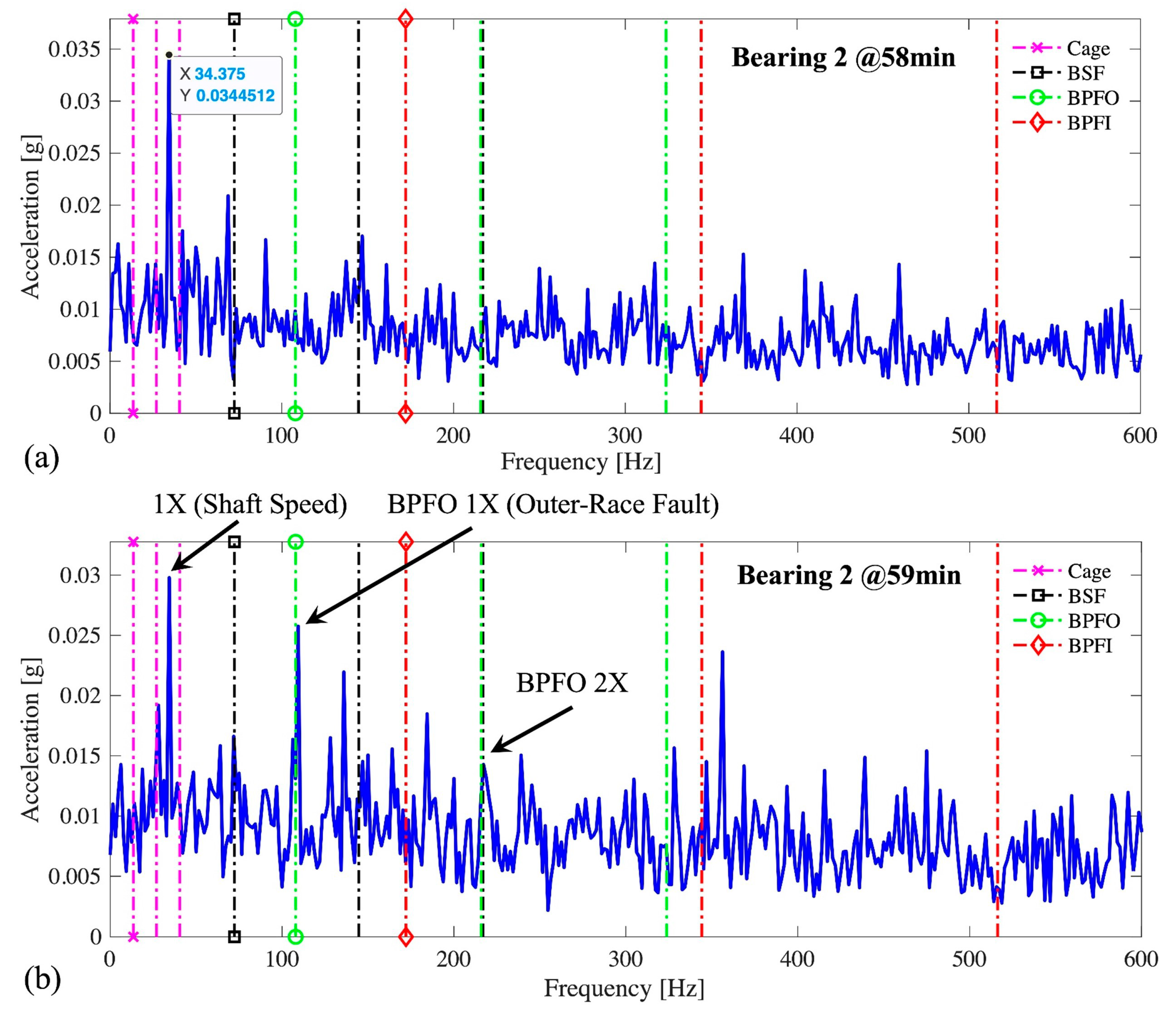
4.1. Fault Detection Based on Averaged Envelope Spectrum

As the radial force of test bearing is imposed with a hydraulic loading from the horizontal direction, the raw vibration signals of the horizontal accelerometers are utilized for further analysis; they are shown in Figure 5.

In order to identify faults in each bearing at an early stage, the proposed averaged envelope spectrum is calculated according to Section 3.1.2 for each acceleration signal during the experiment. Subsequently, a spectral inspection is carried out on each envelope spectrum to pinpoint the bearing’s fault characteristic frequencies. This process is performed for every signal measurement throughout the bearing’s lifespan which helps in identifying the initiation of the bearing fault and facilitates the generation of a precise detection time $t_{FDT}$ for the further prediction of RUL.

The results of the fault detection are summarized in

Table 4. Results of bearing fault detection based on envelope spectrum inspection.

Operating Condition (Speed/Load)	Bearing ID	First Detection Time of Fault ${\mathit{t}}_{\mathit{F}\mathit{D}\mathit{T}}$	End-of-Life Time ${\mathit{t}}_{\mathit{E}\mathit{O}\mathit{L}}$	Fault Type
C1: 35Hz/12kN	1 2	35 min 59 min	126 min 151 min	Outer-Race Fault Outer-Race Fault
C2: 37.5Hz/11kN	3 4	446 min 47 min	490 min 160 min	Inner-Race Fault Outer-Race Fault
C3: 40Hz/10kN	5 6	327 min 1418 min	353 min 1478 min	Inner-Race Fault Inner-Race Fault

, where $t_{FDT}$ denotes the first detection time of faults and the bearing EOL time is further discussed in Section 4.2. For illustration, Figure 6, Figure 7 and Figure 8 present the spectral changes during the initial detection of a bearing fault for Bearings 2, 4 and 6, marking the transition from the healthy state to the degradation stage.

As shown in Figure 6, the vibration signals of Bearing 2 at the 58th and the 59th minute are both dominated by the frequency component at the shaft speed. However, the peaks at the BPFO and its second multiple become more prominent in the latter spectrum (Figure 6b). Despite the weaker energy compared to the rotation frequency (’1X’), the BPFO components indicate the onset of the outer-race fault which occurs after the 59th minute during the run-to-failure experiment.

Similarly, the spectral variations at the fault initiation of Bearing 4 are presented in Figure 7. It is seen that the envelope spectrum of the 46th minute is dominated by the shaft rotation frequency (Figure 7a), whereas the frequency components at the BPFO and its harmonic intensify and dominate the envelope spectrum at the 47th minute. With further inspection of the full life-cycle data, it is verified that the outer-race fault has manifested in Bearing 4 since the 47th minute.

Likewise, Figure 8 shows the envelope spectra during the fault onset for Bearing 6. It is seen that the envelope spectrum in Figure 8a is governed by the shaft speed but also masked with random components. However, although dominated by the shaft rotation frequency, the envelope spectrum at the 1418th minute exhibits evident frequency components at the BPFI and its second multiple. Furthermore, the presence of sidebands at the synchronous speed (‘1X’) suggests a strong modulation of the BPFI by the shaft speed, which indicates the occurrence of the inner-race fault in Bearing 6 since the 1418th minute.

4.2. Envelope Spectral Indicators

Based on the results of the averaged envelope spectrum, the bearing fault characteristic frequencies can be identified, the spectrum amplitudes of which are combined to compute the proposed ESI for measuring the bearing degradation level. Accordingly, the ESIs of the test bearings are shown in Figure 9. For each test bearing, the first detection time of faults, $t_{FDT}$, identified based on the inspection of the averaged envelope spectrum, is marked by the black dotted line.

It is seen that each of the ESI plots maintains a stable platform at the healthy stage while exhibiting an overall ascending trajectory from the time when the bearing fault initiates, indicative of an accelerating trend of bearing degradation. However, it is noteworthy that these ESIs are not strictly monotonic and display substantial fluctuations as they approach the end of machine operation. Except Bearings 3 and 4, the ESI trajectories of other test bearings show noticeable declines at the end of the experiments. This could be explained by the theory of ’healing phenomena’ during the bearing deterioration [5], where the defect surfaces caused by wear or fatigue may partially restore the original smoothness due to several potential factors such as the redistribution of lubrication or the removal of debris, leading to a small performance improvement in friction and vibration. However, it should be noted that this phenomenon does not guarantee the prevention of subsequent degradation.

As a representation of the functional failures of rolling bearings, the end-of-life time is formulated as the time when the extracted ESI reaches the maximum, indicating the peak energy of the vibration components at the FCFs, as defined in Equation (4). Respectively, the end-of-life time $t_{EOL}$ for each bearing is listed in Table 4 and marked with a black dashed line in Figure 9.

Based on the computation of the ESI for all the available test bearings, the average level of the ESI at $t_{EOL}$ is utilized as the failure threshold for further prediction of RUL, which is $\overline{\gamma }=3.24$.

4.3. RUL Prediction of Test Bearings under Condition C1

Once the early fault is detected, the EKF is applied to estimate the latent degradation level of bearings for RUL prediction. As defined in Section 3.4.3, the degradation state of the test bearing is assumed to follow an accelerating increasing trend before reaching the average end-of-life threshold $\overline{\gamma }$.

In Figure 10a, the degradation-stage ESI of Bearing 1 is presented as a grey solid line. The first detection time of fault $t_{FDT}$ is the 35th minute as marked by the black dotted line. Observations reveal that the ESI after $t_{FDT}$ exhibits a gradual upward trend with more fluctuation at the later time. The maximum value of ESI corresponds to the end-of-life time of Bearing 1 ($t_{EOL}=126$) as represented by the red dash-dot line, indicative of the need for replacement. Considering the uncertainty in the initial states, 10 additional data points preceding $t_{FDT}$ are incorporated to update the state estimations in the EKF. Henceforth, the ESIs starting from the 25th minute, specifically marked with red circles, are utilized for the EKF-based RUL prediction model.

After initializing the model according to Section 3.4.4 and setting the noise levels empirically as $v_t=0.1$, $w_t=0.05$, the EKF algorithm is implemented for degradation state estimation until the prediction time $t_{PT}$, at which the estimated failure time ${\tilde{t}}_{EOL}$ is predicted based on the state extrapolation and the average EOL threshold $\overline{\gamma }$. Figure 10a–d show the extrapolation results of the bearing degradation state at four prediction times: the 40th, 45th, 50th and 55th minutes, which are, respectively 5, 10, 15 and 20 minutes after the fault detection. It can be observed that the estimated EOL time, ${\tilde{t}}_{EOL}$, in each prediction is closely in the vicinity of the baseline, $t_{EOL}$.

As for Bearing 2, Figure 11 demonstrates that the ESI of the bearing follows an accelerating increasing pattern, reaching the maximum at the 151st minute. An outer-race fault is detected at the 59th minute based on the spectral inspection results of envelope analysis (see Section 4.1). Similarly, the ESI data from the 49th minute (marked with red circles) are employed for state estimation in the EKF algorithm. Using the noise levels at $v_t=0.1$, $w_t=0.05$, the estimated EOL time at various predicting times can be obtained.

Figure 11a–d present the results of four $t_{PT}$ at the 66th, 69th, 71st and 74th minutes. It is observed that despite the early prediction at the 66th minute in Figure 11a, the prediction of the EOL time ${\tilde{t}}_{EOL}$ in Figure 11b is exactly the same as the baseline EOL time, and that the extrapolations of ${\tilde{t}}_{EOL}$ at the later times are also accurate, as in Figure 11c,d.

To evaluate the performance of the proposed method for bearing RUL prediction, the state estimation results with uncertainty estimation for Bearings 1 and 2 are summarized in

Table 5. RUL Prediction Results of Bearing 1 and Bearing 2 (Condition 1).

Bearing ID	Baseline $\mathbf{FDT}*{\mathit{t}}_{\mathit{F}\mathit{D}\mathit{T}}$/minute	Baseline $\mathbf{EOLT}*{\mathit{t}}_{\mathit{E}\mathit{O}\mathit{L}}$/minute	$\mathbf{RUL}\mathbf{PT}*{\mathit{t}}_{\mathit{P}\mathit{T}}$/minute	Estimated End-of-Life Time ${\tilde{\mathit{t}}}_{\mathit{E}\mathit{O}\mathit{L}}$/minute	Baseline RUL /minute	Estimated RUL (Residual) /minute	RUL 95% CI /minute
1	35	126	40	127	86	87 (+1)	[84,89]
			45	126	81	81 (0)	[79,83]
			50	134	76	84 (+8)	[83,87]
			55	111	71	56 (−15)	[56,63]
2	59	151	66	146	85	80 (−5)	[70,88]
			69	151	82	82 (0)	[74,91]
			71	149	80	78 (−2)	[70,85]
			74	150	77	76 (−1)	[69,83]

* Baseline FDT: first detection time of fault. Baseline EOLT: bearing end-of-life time of ground truth. PT: RUL prediction time.

. The result shows that the established degradation model well expresses the initial upward trend in the ESI during the early stage of bearing degradation using one dynamic model parameter, $b_t$. It also demonstrates that the EKF algorithm is capable of estimating the RUL of bearings with a few ESI data points since the first detection of faults.

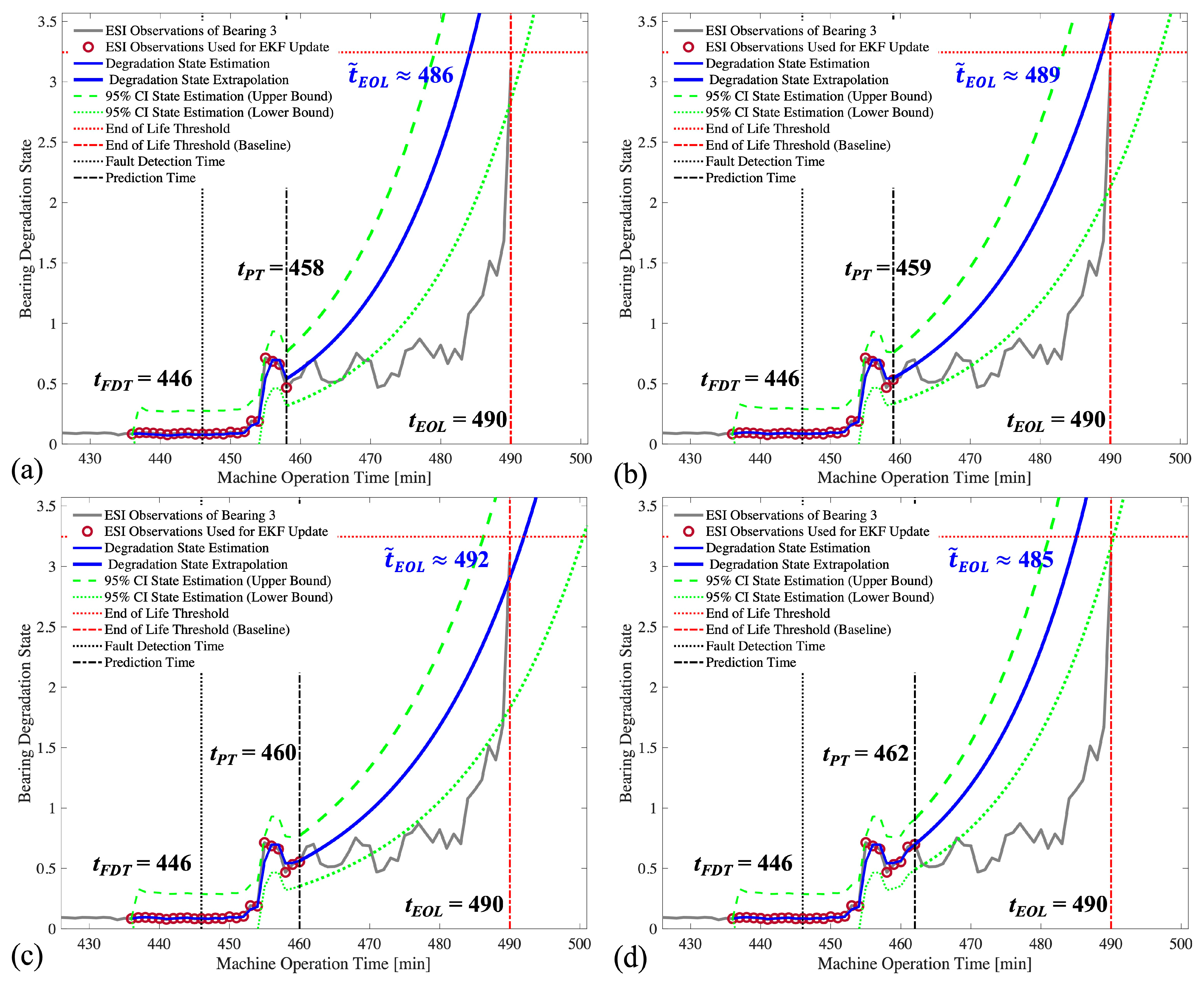
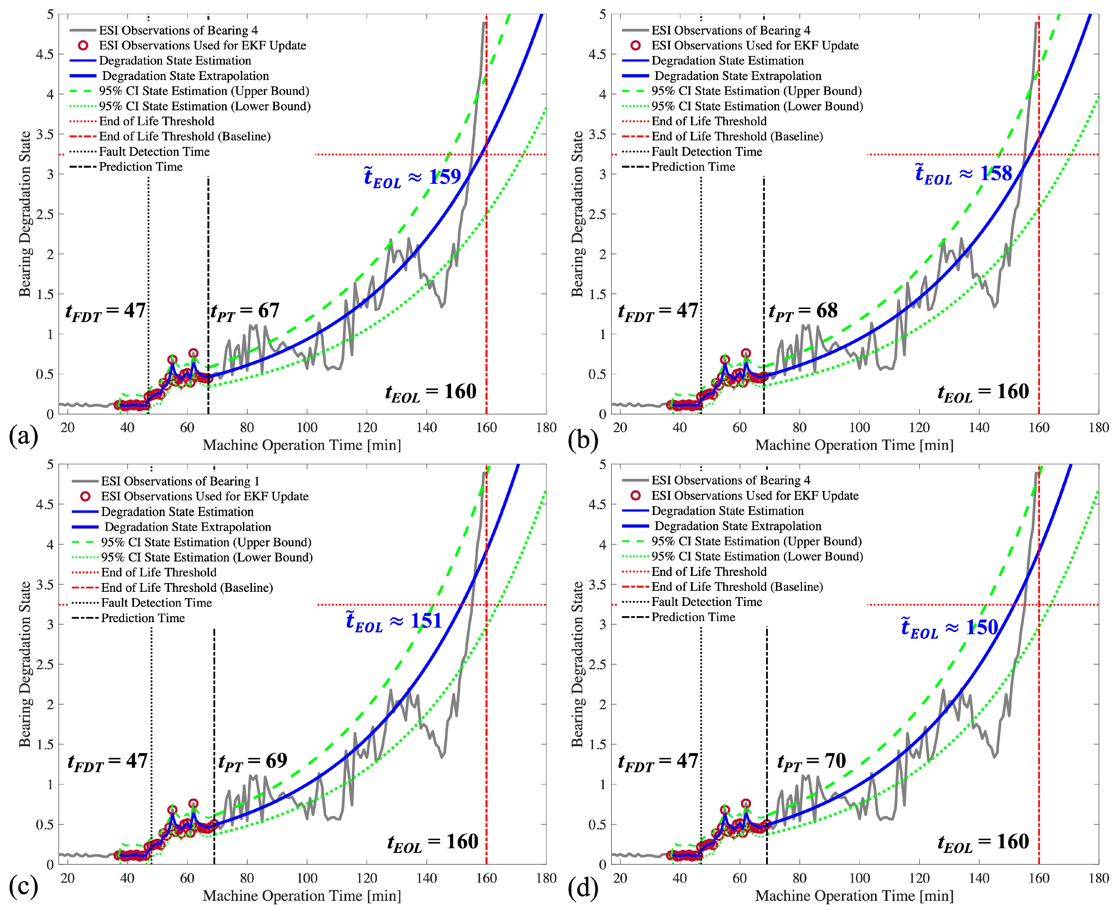
4.4. RUL Prediction of the Test Bearings under Condition C2

To validate the prediction performance of the proposed method, the bearings under Condition 2 are analyzed, in which the shaft speed is 37.5 Hz with the loading at 11 kN. The EKF model is further applied to the ESI of Bearings 3 and 4 for RUL prediction at the early stage of bearing degradation.

According to the envelope analysis results in Table 4, the presence of the inner-race fault is identified in Bearing 3 after 446 minutes. Then, the ESI data from the 436th minute to the RUL prediction time $t_{PT}$ are employed for the degradation state estimation using the proposed EKF models. The state process noise and the measurement noise are, respectively, set as $v_t=0.02$, $v_t=0.05$. After recursive filtering using the ESI observations (marked with a red circle in Figure 12), the estimated EOL time ${\tilde{t}}_{EOL}$ at the prediction time can be extrapolated based on the updated state at $t_{PT}$ according to (38). Four predictions within 20 minutes after the fault is detected ($t_{FDT}$) are shown in Figure 12.

In the prediction result, an evident surge in the ESI of Bearing 3 is observed following the initiation of a fault. This surge results in the prediction of an early failure time at ${\tilde{t}}_{EOL}=486$, which is extrapolated from the state estimation at $t_{PT}=458$, as in Figure 12a. Meanwhile, the further predictions of the EOL time at $t_{PT}=459$ and $t_{PT}=460$ (Figure 12b,c) are well projected to the vicinity of the baseline EOL time at $t_{EOL}=$ 490. Overall, the 95% credible intervals of the four predictions provided in the green dashed lines consistently cover the baseline end-of-life time.

Analogously, Figure 13 displays the state estimation results by applying the EKF algorithm for the ESI of Bearing 4. The noise levels for the state process and the observations are, respectively, set at $v_t=0.05$, $w_t=0.08$. Notably, the state extrapolation at different prediction times effectively represents the overall pattern of the ESI (in the grey solid line). The predicted end-of-life times at $t_{PT}=67$ minute and $t_{PT}=68$ minute are estimated, respectively, as ${\tilde{t}}_{EOL}=159$ minute and ${\tilde{t}}_{EOL}=158$ minute, which closely correspond to the baseline end-of-life time at $t_{EOL}=160$ minute.

For the assessment of the prediction accuracy, the state estimation results and the corresponding RUL are provided in

Table 6. RUL Prediction Results of Bearing 3 and Bearing 4 (Condition 2).

Bearing ID	Baseline FDT*${\mathit{t}}_{\mathit{F}\mathit{D}\mathit{T}}$ /minute	Baseline $\mathbf{EOLT}*{\mathit{t}}_{\mathit{E}\mathit{O}\mathit{L}}$ /minute	$\mathbf{RUL}\mathbf{PT}*{\mathit{t}}_{\mathit{P}\mathit{T}}$ /minute	Estimated End-of-Life Time ${\tilde{\mathit{t}}}_{\mathit{E}\mathit{O}\mathit{L}}$ /minute	Baseline RUL /minute	Estimated RUL (Residual) /minute	RUL 95% CI /minute
3	446	490	458	486	32	28 (−4)	[21,34]
			459	489	31	30 (−1)	[24,38]
			460	492	30	32 (+2)	[26,41]
			462	485	28	23 (−5)	[19,28]
4	47	160	67	159	93	92 (−1)	[80,105]
			68	158	92	90 (−2)	[78,102]
			69	151	91	82 (−9)	[73,95]
			70	150	90	80 (−10)	[71,91]

* Baseline FDT: first detection time of fault. Baseline EOLT: bearing end-of-life time of ground truth. PT: RUL prediction time.

, where the mean estimated RUL, the residuals between the estimated RUL and the baseline RUL, and the 95% credible intervals are summarized. It is seen that the overall prediction of RUL is fairly accurate and tends to be conservative given the negative residuals of the RUL estimate. Also, the absolute errors of the predicted RUL are no more than 5 minutes for Bearing 3, where the predicting times of the RUL are within 20 minutes after the fault detection. In addition, for Bearing 4, the absolute errors of the RUL prediction are less than 10 minutes with the predicting time of the RUL at around 20 minutes after the fault is detected.

4.5. Further Validation on the Test Bearings under Condition C3

Next, further validation is introduced to the test bearings operating under condition 3, where the shaft speed is 40 Hz with 10 kN hydraulic loading.

For Bearing 5, the ESI exhibits a steady plateau before the inner-race fault is found at the 327th minute, after which it surges rapidly to the maximum value at the 353rd minute. This indicates that Bearing 5 undergoes a rapid degradation stage that lasts for merely 26 minutes. Based on the EKF algorithm outlined in Section 3.4.4, the bearing end-of-life time can be estimated using the ESI observations from the 327th minute to the various prediction times, $t_{PT}$. With the noise levels of the state process and the measurement set at $v_t=0.1$ and $w_t=0.1$, the results of the state estimation and further extrapolation based on the EKF are shown in Figure 14.

As for Bearing 6, after the detection of the inner-race fault at the 1418th minute ($t_{FDT}$ = 1418), the ESI observations since the 1407th minute (as marked with red circles in Figure 15) are used for degradation state estimation in the EKF. It is seen that the state extrapolation captures the overall increasing trend of the ESI and provides a fairly precise estimate of end-of-life time, ${\tilde{t}}_{EOL}$.

For performance evaluation, the RUL at the prediction time of Bearings 5 and 6 are summarized in

Table 7. RUL Prediction Results of Bearing 5 and Bearing 6 (Condition 3).

Bearing ID	Baseline $\mathbf{FDT}*{\mathit{t}}_{\mathit{F}\mathit{D}\mathit{T}}$ /minute	Baseline $\mathbf{EOLT}*{\mathit{t}}_{\mathit{E}\mathit{O}\mathit{L}}$ /minute	$\mathbf{RUL}\mathbf{PT}*{\mathit{t}}_{\mathit{P}\mathit{T}}$ /minute	Estimated End-of-Life Time ${\tilde{\mathit{t}}}_{\mathit{E}\mathit{O}\mathit{L}}$	Baseline RUL /minute	Estimated RUL (Residual) /minute	RUL 95% CI /minute
5	327	353	343	355	10	12 (+2)	[10,14]
			345	350	8	5 (−3)	[4,6]
			346	349	7	3 (−4)	[2,4]
			347	352	6	5 (−1)	[4,6]
6	1418	1478	1428	1472	50	44 (−6)	[38,50]
			1429	1476	49	47 (−2)	[41,53]
			1430	1477	48	47 (−1)	[41,54]
			1441	1478	37	37 (0)	[33,41]

* Baseline FDT: first detection time of fault. Baseline EOLT: bearing end-of-life time of ground truth. PT: RUL prediction time.

. For Bearing 5, it can be concluded that the absolute residuals of the predicted RUL are less than 5 minutes. As the degradation state represented by the ESI steeply rises to approach the end-of-life threshold, a prompt replacement is suggested for Bearing 5 to avoid critical failures.

As for Bearing 6, the estimated RULs at the prediction times $t_{PT}=1428$ and $t_{PT}=1429$ are close to but earlier than their baselines. Note that the prediction times are merely about 10 minutes away from the detection of fault. Additionally, the RUL estimations at $t_{PT}=1430$ and $t_{PT}=1441$ are more precise since their residuals have reduced to less than one minute.

5. Discussion

As mentioned in Section 1, the pure physics-based models for RUL prediction are beneficial when a clear understanding of the failure mechanism is available, while the deterioration dynamics of the bearing is not yet fully unveiled and often in practice, not all the prior physics information (e.g., defect dimension) is available. Therefore, the prediction accuracy of the pure physics-based methods may be limited in practical applications. In general, the pure data-driven approaches and statistical approaches are not strictly separated. Although pure statistics methods (e.g., survival analysis) may require a large amount of historical data that provide consistent statistical meaningful results, such as the data requirement in pure data-driven approaches (e.g., neural networks) to ensure generalization performance, both have this advantage: no detailed knowledge of the failure mechanism is needed.

In this study, the recursive Bayesian filter is applied combining the advantages of both physics-based and data-driven approaches. The envelope spectral indicator is crafted relating to bearing fault characteristics and is incorporated to the EKF for sequential estimation of the bearing degradation state with uncertainty estimation.

The experimental results on the test bearings under various operating conditions have demonstrated promising performance of the ESI in representing the bearing degradation process and the EKF in RUL prediction. In the above cases, the EKF-based RUL predictions at the discrete time steps shortly after the fault detection exhibit commendable accuracy and precision. The prediction results suggest that the EKF could effectively integrate the bearing ESI data and update the state estimation, which underscores the capability of the proposed model to capture short-term trends and variations in the ESI during bearing deterioration, providing valuable insights into the impending failure and the RUL of bearings.

On the other hand, it is also important to acknowledge that the prediction based on more ESI observations may exhibit a more intricate pattern. In the cases of continuous RUL prediction, it is justifiable to claim that there is a convergence of prediction accuracy towards the end of the bearing life because of the health indicators approaching the pre-specified end-of-life threshold. Yet, the significance of the late-stage RUL predictions might be diminished due to their proximity to the bearing failure, thereby limiting their practical value for maintenance decision making. In contrast, the significance of the presented method is highlighted for the ability to provide meaningful RUL predictions during the early phase of the bearing degradation.

Regarding the computation cost of the proposed methods, the proposed averaged envelope spectrum can be efficiently computed based on the Hilbert transform and the fast Fourier transform. As for the EKF, the state process model for the bearing degradation has been further optimized and only one-dimensional measurement is leveraged. Also, the study targets the early phase RUL prediction by using only a few observations of the health indicators at the fault detection phase, which results in low computation requirements.

In summary, the effectiveness of the EKF-based RUL prediction methodology has been demonstrated on the experimental bearing vibration data of various operating conditions. The bearing RUL can be predicted shortly after the fault detection based on the ESI at the early phase of bearing degradation. The findings collectively highlight the promising potentials of the proposed method combining the ESI and the EKF for the early prediction of RUL, which contributes to the practical implementation of advanced condition monitoring and predictive maintenance methodologies.

6. Conclusions

The presented work proposes the envelope spectral indicator combining the vibration energy of the bearing fault characteristic frequencies to closely represent the bearing degradation state, and utilizes the extended Kalman filter algorithm for the degradation state estimation given only a few ESI observations about the fault detection time. The proposed ESI is formulated based on the bearing FCF components in the averaged envelope spectrum, which is enhanced against the random noise through the PSD of the envelope signal segments. The ESI is beneficial in representing the latent deterioration condition of rolling-element bearings as the constituting components of the ESI are solely related to the bearing defects. This indicates that the ESI is free of the interference from the synchronous speed component and the fault components arising from the coupled mechanical structures such as rotors and gear pairs. Along with the computation of ESI, the bearing fault can be efficiently identified through the spectral inspection of the averaged envelope spectrum.

On the above basis, the early RUL prediction approach for REBs is achieved based on the combination of ESI and EKF. Once the fault is detected in the bearing, only a small number of the ESI observations from the early degradation process are employed for degradation state estimation and end-of-life time prediction. The predictive performance is validated on the public experimental vibration data measured from a bearing rig. The thorough results and observations presented have demonstrated the efficacy of the proposed method for predicting the RUL of rolling bearings even at the early stage of degradation. Therefore, by enabling the early detection and prediction of RUL, the proposed method may foster more efficient and cost-effective maintenance practices and is identified as having great potential to optimize predictive maintenance strategies for engineering practice.

References

1. Dupuis, R. Application of Oil Debris Monitoring for Wind Turbine Gearbox Prognostics and Health Management. Annu. Conf. PHM Soc. 2010, 2, 1–15. [Google Scholar]
2. Liang, L.; Ding, X.; Wen, H.; Liu, F. Impulsive Components Separation Using Minimum-Determinant KL-Divergence NMF of Bi-Variable Map for Bearing Diagnosis. Mech. Syst. Signal Process. 2022, 175, 109129. [Google Scholar] [CrossRef]
3. Si, X.S.; Wang, W.; Hu, C.H.; Zhou, D.H. Remaining Useful Life Estimation—A Review on the Statistical Data Driven Approaches. Eur. J. Oper. Res. 2011, 213, 1–14. [Google Scholar] [CrossRef]
4. Lienig, J.; Bruemmer, H. Reliability Analysis. In Fundamentals of Electronic Systems Design; Springer International Publishing: Cham, Switzerland, 2017; pp. 45–73. [Google Scholar]
5. Qiu, H.; Lee, J.; Lin, J.; Yu, G. Wavelet Filter-Based Weak Signature Detection Method and Its Application on Rolling Element Bearing Prognostics. J. Sound Vib. 2006, 289, 1066–1090. [Google Scholar] [CrossRef]
6. Nectoux, P.; Gouriveau, R.; Medjaher, K.; Ramasso, E.; Morello, B.; Zerhouni, N.; Varnier, C. PRONOSTIA: An Experimental Platform for Bearings Accelerated Degradation Tests. In Proceedings of the IEEE International Conference on Prognostics and Health Management, PHM’12, Denver, CO, USA, 18–21 June 2012. [Google Scholar]
7. Wang, B.; Lei, Y.; Li, N.; Li, N. A Hybrid Prognostics Approach for Estimating Remaining Useful Life of Rolling Element Bearings. IEEE Trans. Reliab. 2020, 69, 401–412. [Google Scholar] [CrossRef]
8. Poplawski, J.V.; Peters, S.M.; Zaretsky, E.V. Effect of Roller Profile on Cylindrical Roller Bearing Life Prediction—Part I: Comparison of Bearing Life Theories. Tribol. Trans. 2008, 44, 339–350. [Google Scholar] [CrossRef]
9. International Organization for Standardization ISO 281:2007 Rolling Bearings: Dynamic Load Ratings and Rating Life. Available online: https://www.iso.org/standard/38102.html (accessed on 11 July 2023).
10. Zaretsky, E.V. Rolling Bearing Life Prediction, Theory, and Application; NASA Tech. Reports 2013, No. NASA/TP-2013-215305; NASA: Washington, DC, USA, 2013. [Google Scholar]
11. Loutas, T.H.; Roulias, D.; Georgoulas, G. Remaining Useful Life Estimation in Rolling Bearings Utilizing Data-Driven Probabilistic E-Support Vectors Regression. IEEE Trans. Reliab. 2013, 62, 821–832. [Google Scholar] [CrossRef]
12. Alfarizi, M.G.; Tajiani, B.; Vatn, J.; Yin, S. Optimized Random Forest Model for Remaining Useful Life Prediction of Experimental Bearings. IEEE Trans. Ind. Inform. 2023, 19, 7771–7779. [Google Scholar] [CrossRef]
13. Mao, W.; He, J.; Zuo, M.J. Predicting Remaining Useful Life of Rolling Bearings Based on Deep Feature Representation and Transfer Learning. IEEE Trans. Instrum. Meas. 2020, 69, 1594–1608. [Google Scholar] [CrossRef]
14. Wang, H.; Ma, X.; Zhao, Y. An Improved Wiener Process Model with Adaptive Drift and Diffusion for Online Remaining Useful Life Prediction. Mech. Syst. Signal Process. 2019, 127, 370–387. [Google Scholar] [CrossRef]
15. Li, Y.; Huang, X.; Ding, P.; Zhao, C. Wiener-Based Remaining Useful Life Prediction of Rolling Bearings Using Improved Kalman Filtering and Adaptive Modification. Meas. J. Int. Meas. Confed. 2021, 182, 109706. [Google Scholar] [CrossRef]
16. Singleton, R.K.; Strangas, E.G.; Aviyente, S. Extended Kalman Filtering for Remaining-Useful-Life Estimation of Bearings. IEEE Trans. Ind. Electron. 2015, 62, 1781–1790. [Google Scholar] [CrossRef]
17. Mosallam, A.; Medjaher, K.; Zerhouni, N. Data-Driven Prognostic Method Based on Bayesian Approaches for Direct Remaining Useful Life Prediction. J. Intell. Manuf. 2016, 27, 1037–1048. [Google Scholar] [CrossRef]
18. Särkkä, S. Bayesian Filtering and Smoothing; Cambridge University Press: Cambridge, UK, 2013; ISBN 9781107030657. [Google Scholar]
19. Andrade-Cetto, J. The Kalman Filter. Tech. Rep. Inst. Robot. i Inform. Ind. 2002. CSIC-UPC (IRI-DT-02-01). Available online: https://www.iri.upc.edu/publications/show/545 (accessed on 1 May 2023).
20. Haykin, S. Kalman Filtering and Neural Networks; Wiley: Hoboken, NJ, USA, 2001; Volume 5, ISBN 9780471369981. [Google Scholar]
21. Wan, E.A.; Van Der Merwe, R. The Unscented Kalman Filter for Nonlinear Estimation. In Proceedings of the IEEE 2000 Adaptive Systems for Signal Processing, Communications, and Control Symposium (Cat. No.00EX373), Lake Louise, AB, Canada, 4 October 2000; pp. 153–158. [Google Scholar] [CrossRef]
22. Coelho, M.d.F.; Bousson, K.; Ahmed, K. An Improved Extended Kalman Filter for Radar Tracking of Satellite Trajectories. Designs 2021, 5, 54. [Google Scholar] [CrossRef]
23. Singh, M.; Lakra, S.; Das, S.; Mishra, S.K.; Sahoo, A.K.; Acharya, B. Extended Kalman Filter-Based Position Estimation in Autonomous Vehicle Applications. Lect. Notes Electr. Eng. 2023, 887, 427–440. [Google Scholar] [CrossRef]
24. Liang, L.; Wen, H.; Liu, F.; Li, G.; Li, M. Feature Extraction of Impulse Faults for Vibration Signals Based on Sparse Non-Negative Tensor Factorization. Appl. Sci. 2019, 9, 3642. [Google Scholar] [CrossRef]
25. Wen, H.; Zhang, L.; Sinha, J.K. Adaptive Band Extraction Based on Low Rank Approximated Nonnegative Tucker Decomposition for Anti-Friction Bearing Faults Diagnosis Using Measured Vibration Data. Machines 2022, 8, 694. [Google Scholar] [CrossRef]
26. Randall, R.B.; Antoni, J. Rolling Element Bearing Diagnostics—A Tutorial. Mech. Syst. Signal Process. 2011, 25, 485–520. [Google Scholar] [CrossRef]
27. Sinha, J.K. Vibration Analysis, Instruments, and Signal Processing; CRC Press: Boca Raton, FL, USA, 2014; ISBN 9781482231458. [Google Scholar]
28. Dai, Y.; Yu, S.; Yan, Y.; Yu, X. An EKF-Based Fast Tube MPC Scheme for Moving Target Tracking of a Redundant Underwater Vehicle-Manipulator System. IEEE/ASME Trans. Mechatron. 2019, 24, 2803–2814. [Google Scholar] [CrossRef]
29. Feng, D.; Wang, C.; He, C.; Zhuang, Y.; Xia, X.-G. Kalman-Filter-Based Integration of IMU and UWB for High-Accuracy Indoor Positioning and Navigation. IEEE Internet Things J. 2020, 7, 3133–3146. [Google Scholar] [CrossRef]
30. Lei, Y.; Xia, D.; Erazo, K.; Nagarajaiah, S. A Novel Unscented Kalman Filter for Recursive State-Input-System Identification of Nonlinear Systems. Mech. Syst. Signal Process. 2019, 127, 120–135. [Google Scholar] [CrossRef]
31. Batzel, T.D.; Swanson, D.C. Prognostic Health Management of Aircraft Power Generators. IEEE Trans. Aerosp. Electron. Syst. 2009, 45, 473–483. [Google Scholar] [CrossRef]
32. Sepasi, S.; Ghorbani, R.; Liaw, B.Y. Improved Extended Kalman Filter for State of Charge Estimation of Battery Pack. J. Power Sources 2014, 255, 368–376. [Google Scholar] [CrossRef]
33. Simon, D. Optimal State Estimation: Kalman, H∞, and Nonlinear Approaches; Wiley: Hoboken, NJ, USA, 2006; ISBN 9780471708582. [Google Scholar] [CrossRef]
Figure 1. The schematic diagram of the experimental rig (reorganized from [7]).
Applsci 14 00436 g001
Figure 2. A typical example of the envelope spectrum with multiple bearing FCFs.
Applsci 14 00436 g002
Figure 3. An example of bearing degradation process. Bearing health indicator vs. operation time. The bearing lifetime is typically divided into the healthy stage and the degradation stage.
Applsci 14 00436 g003
Figure 4. The overall procedure of the EKF-based RUL prediction method.
Applsci 14 00436 g004
Figure 5. The horizontal acceleration signals of the analyzed test bearings: (af): Bearings 1 to 6.
Applsci 14 00436 g005
Figure 6. The averaged envelope spectra indicating the fault initiation of Bearing 2: (a) The envelope spectrum at the 58th minute. (b) The envelope spectrum at the 59th minute, where the outer-race fault is identified.
Applsci 14 00436 g006
Figure 7. The averaged envelope spectra indicating the fault initiation of Bearing 4: (a) The envelope spectrum at the 46th minute. (b) The envelope spectrum at the 47th minute when the outer-race fault is identified.
Applsci 14 00436 g007
Figure 8. The averaged envelope spectra indicating the fault initiation of Bearing 6: (a) The envelope spectrum at the 1417th minute. (b) The envelope spectrum at the 1418th minute when the inner-race fault is identified.
Applsci 14 00436 g008
Figure 9. The envelope spectral indicator (ESI) of bearing degradation state: (af): Bearings 1 to 6. (Blue dotted scatter plot: the extracted ESI. Red solid line: the smoothed ESI using 4-point moving average).
Applsci 14 00436 g009
Figure 10. Bearing 1 degradation state prediction based on the EKF: (a) State prediction at the 40th minute. The corresponding estimated RUL is = 87 r u l ~ 40 = t ~ E O L t P T = 87 minutes. (b) State prediction at the 45th minute, with r u l ~ 45 = 81 minutes. (c) State prediction at the 50th minute, with r u l ~ 50 = 84 minutes. (d) State prediction at the 55th minute, with r u l ~ 55 = 56 minutes.
Applsci 14 00436 g010
Figure 11. Bearing 2 degradation state prediction based on the EKF: (a) State prediction at the 66th minute. The corresponding estimated RUL is r u l ~ 66 = t ~ E O L t P T = 80 minutes. (b) State prediction at the 69th minute, with r u l ~ 69 = 82 minutes. (c) State prediction at the 71st minute, with r u l ~ 71 = 78 minutes. (d) State prediction at the 74th minute, with r u l ~ 74 = 76 minutes.
Applsci 14 00436 g011
Figure 12. Bearing 3 degradation state prediction based on the EKF: (a) State prediction at the 458th minute. The corresponding estimated RUL is r u l ~ 458 = t ~ E O L t P T = 28 minutes. (b) State prediction at the 459th minute, with r u l ~ 459 = 30 minutes. (c) State prediction at the 460th minute, with r u l ~ 460 = 32   minutes. (d) State prediction at the 462nd minute, with r u l ~ 462 = 23 minutes.
Applsci 14 00436 g012
Figure 13. Bearing 4 degradation state prediction based on the EKF: (a) State prediction at the 67th minute. The corresponding estimated RUL is r u l ~ 67 = t ~ E O L t P T = 92 minutes. (b) State prediction at the 68th minute, with r u l ~ 68 = 90 minutes. (c) State prediction at the 69th minute, with r u l ~ 69 = 82   minutes. (d) State prediction at the 70th minute, with r u l ~ 70 = 80 minutes.
Applsci 14 00436 g013
Figure 14. Bearing 5 degradation state prediction based on the EKF: (a) State prediction at the 343rd minute. The corresponding estimated RUL is r u l ~ 343 = t ~ E O L t P T = 12 minutes. (b) State prediction at the 345th minute, with r u l ~ 345 = 5 minutes. (c) State prediction at the 346th minute, with r u l ~ 346 = 3   minutes. (d) State prediction at the 347th minute, with r u l ~ 347 = 5 minutes.
Applsci 14 00436 g014
Figure 15. Bearing 6 degradation state prediction based on the EKF: (a) State prediction at the 1428th minute. The corresponding estimated RUL is r u l ~ 1428 = t ~ E O L t P T = 44 minutes. (b) State prediction at the 1429th minute, with r u l ~ 1429 = 47 minutes. (c) State prediction at the 1430th minute, with r u l ~ 1430 = 47   minutes. (d) State prediction at the 1441st minute, with r u l ~ 1441 = 37 minutes.
Applsci 14 00436 g015