Modification of Genetic Algorithm Based on Extinction Events and Migration

Abstract

This article presents a genetic algorithm modification inspired by events related to great extinctions. The main objective of the modification was to minimize the number of objective function solutions until the minimum for the function was established. It was assumed that, within each step, a population should be smaller than that recommended in the applicable literature, the number of iterations should be limited, the solution area should be variable, and a great extinction event should take place following several iterations. Calculations were performed for 10 individuals within a population, 10 iterations, two generations each, with a great extinction event happening once every three iterations. The developed algorithm was presented, capable of indicating the minimum number of Eggholder and Rastrigin functions, with a higher probability than the master algorithm (default “ga” in MATLAB) at the same number of objective function solutions. An algorithm was proposed focusing on minimizing the randomization of the objective function, which may be an alternative to the surrogate model. Typically, the emphasis is on achieving as much accuracy as possible. This article presents a method for minimizing the randomization of the objective function and obtaining the highest possible accuracy. A method is presented which minimizes the disadvantages of the largest computation time and the need to generate many samples for typical genetic algorithms (GAs). Optimization results for the classic GA, GEGA, WOA, SMA, and SSA algorithms for the Eggholder and Rastrigin functions were compared. A modification of the genetic algorithm was made to obtain a global extreme with satisfactory accuracy and a sufficiently high probability, while minimizing the number of samples calculated on the basis of the objective function. The developed methodology was used to fulfill the target function for the turbine disc.

1. Introduction

Nowadays, due to the need to achieve high efficiency, engineering problems require optimization in almost every field. For example, the work in [1] used the Support Vector Regression Optimized by the Grasshopper Optimization (SVR-GO) technique to predict gust-induced vibrations. In paper [2], particle swarm optimization (PSO) algorithm was used to control the course maintenance of a ship insufficiently immobilized. In paper [3], optimization of 3D-printed high-speed prototype deep drawing tools was carried out. In [4], optimization of the synthesis of Ag-Cu bimetallic nanoparticles was carried out using a fungus-mediated approach. Based on the DRLDA algorithm, Multi-Train Energy-Saving Control with Urban Rail Transit [5] was optimized. Parameter optimization for an accurate procedure for identifying nonlinear systems using the swept-sine method is presented in paper [6].

The Monte Carlo optimization, which includes the genetic algorithm, requires a significant amount of computing time, in particular when calculating the objective function values or when the limits require solving the equations using the finite element method (FEM) [7] or finite volume method (FVM) [8]. As it was shown in paper [9], PSO is more effective than GA due to a smaller optimization error, shorter run-time, and higher reliability. This paper’s authors suggest modifying the genetic algorithm (GA) through the implementation of events modelled on the great extinctions. GAs are a group of intelligent algorithms initially presented by Holland [10], and based on natural processes of living organism reproduction (crossovers and mutations). Genetic algorithms differ from most commonly utilized algorithms in their initial assumptions. Decision variables are usually encoded in the binary form, and the algorithm uses an objective function directly, rather than its derivatives. The minimum determination process does not start at a single point, such as in gradient methods, but from a certain set of solutions, i.e., the initial population. Moreover, most processes occurring in the algorithm are probabilistic in nature, unlike the majority of the most commonly implemented optimization algorithms. There are numerous GA variations described by authors such as Lee [11] or Katoch [12]. Basic genetic algorithm operators include crossovers and mutations. A crossover involves the exchange of a random proportion of bits between suitably matched individuals (solutions). There are numerous crossover methods, including simulated binary crossover [13], blend crossover [14], arithmetic crossover [15], geometric crossover [16], unimodal normal distribution crossover operator [17], and Laplace crossover [18]. Crossing solutions can also be selected in various ways: roulette methods [19], ranking selection [20], or tournament selection [21]. The population size adjustment methods can also vary. Moreover, the number of offspring may also be variable. Algorithms (1 + 1), (μ + 1), (μ + λ), or (μ,λ) [21] describe how a new, temporary population is created to be later subjected to selection and reduction. A mutation consists of negating a certain number of bits in selected individuals. Genetic algorithms tend to be connected with other optimization methods, such as a Tabu search [22], or light algorithms, such as fuzzy logic [23] or a neural network [24,25]. There have been few attempts to modify the genetic algorithm bases. To modify a population, Jaworski [26] implemented a biological extinction event by removing a certain group of solutions. Jafar-Zanjani [27] presented the Adaptive Genetic Algorithm, in which the classic steps of the genetic algorithm are followed by objective updates to the criteria. So far, the GA has been used in numerous and diverse fields of science. In the paper [28], GA was applied for reactive power optimization purposes, in relation to the optimal power flow problem in power system control planning.

The genetic algorithm is also used as a training algorithm for an artificial neural network with back-propagation [29]. In this paper [30], the genetic algorithm was used to reliably determine a structure with the lowest atomic cluster energy in an arbitrary potential model. Kim at al. [31] applied the genetic algorithm and fuzzy learning to design polymer materials. The GA application examples used here support the thesis according to which the genetic algorithm demonstrates considerable potential, as it is widely used in numerous fields of science. The papers [32,33] presents a genetic algorithm similar to the one presented above in which artificial neural networks were used as surrogate model, to optimize a drum-and-disc turbine engine compressor design. Algorithms that use deep learning are implemented for very detailed blind image quality assessment (BIQA). The development of deep learning algorithms is due to the lack of high-quality algorithms. Techniques based on artificial intelligence methods presented in this work have been used to predict image quality. The applied architecture of artificial neural networks used in the study of the quality of processed data is often associated with a benchmark database. This technique can be used to evaluate the quality of data acquired in real time [34]. The efficiency of applying algorithms using artificial neural networks has become an inherent attribute in applied engineering applications, eliminating the critical technique of positioning observation devices by using efficient algorithms based on artificial network technology for the accurate visual spatial positioning of objects [35].

In the paper [36], the process of algorithm optimization was based on artificial neural networks, which requires the development of efficient structures for locating and classifying observed objects. The research topic of finding perfect algorithms is an important subject in deep data analysis research. The development of technologies based on genetic algorithms has accelerated the development of intelligent and efficient detection structures, and the development of detection and data processing technologies requires the development of comparison methods for algorithms based on artificial neural networks. The method presented in the paper [36], which uses a conventional neural network (CNN) to recognize effective data and process them, required building models of the system and analyzing the factors affecting the performance of the required objective. It should be remembered that any model developed requires testing it and searching for a path aiming at an adequate model. The method we presented can be used to create effective algorithms based on neural networks.

A different approach was proposed in paper [37], where it investigated various factors and conditions that are related to performance and defines a model of a multi-agent system to ensure its improvement. The paper shows that the developed models have a much higher learning performance compared to the Q-Learning algorithm. The summary in the paper clearly shows that there is a need to test algorithms based on comparative models and testing methods, using algorithms based on artificial neural networks to evaluate and detect faults in rotating components. The necessary parameters identifying the operating conditions and their changes were selected for evaluation. To solve the problem, the authors of the paper [38] proposed a method for diagnosing faults and identifying them under different operating conditions of the device. Referring to the methods of diagnosis and use of the proposed algorithm, it can be said that a good approach to verify the effectiveness of the algorithm is the comparative method we proposed. The paper [39] proposed a number of methods based on neural networks. The presented activity recognition model required a special approach to improve identification performance. In the presented method, a major difficulty appeared in the process of manually preparing the class hierarchy when the number of classes is high or when there is little prior knowledge. Although the authors proved the validity of their research, we propose that the efficiency of the algorithms be tested with the proposed tools. Here, the genetic algorithm was additionally modified and numerical examinations were performed on selected test functions.

In addition to genetic algorithms, other algorithms are also used in optimization. For example, paper [40] used the tabu algorithm to optimize industrial cable production scheduling. In papers [41,42], machine learning was used to forecast climate change. In papers [43,44,45,46,47], optimized operational research problems were used. Optimization algorithms are also used in failure mode and effects analysis, as exemplified by the work in [48]. Other algorithms are used to solve complex problems, for example Red Deer Algorithms (RDAs), Social Engineering Optimizer (SEO), Keshtel Algorithm (KA), and particle swarm optimization (PSO).

RDA [49] is a single-point optimization algorithm that works by updating a single solution at a time. The algorithm RDA uses a “deer-inspired” mechanism that maintains diversity by randomizing the step size at each iteration and is more suited for high-dimensional problems as it does not rely on a population of solutions. The works in [50] further the application of RDA to optimization of a multi-echelon sugarcane closed-loop supply chain network.

SEO [51] is an algorithm that incorporates social behavior into the optimization process by considering the influence of neighboring solutions, which it uses to maintain diversity in the population. The modified SEO (MSEO) algorithm [52] was used for optimization. A set of engineering applications were provided to prove and validate the MSEO algorithm for the first time. The experimental outcomes show that the suggested algorithm produces very accurate results, which are better than the SEO and other compared algorithms. Most notably, the MSEO provides a very competitive output and a high convergence rate.

PSO is a swarm-based optimization algorithm that models the behavior of a swarm of particles to find the optimal solution. It uses the velocity of each particle to maintain diversity and balance exploration and exploitation. Studies such as [53,54] are focused on the optimization of jet engine performances witch the PSO algorithm.

Similarly, KA [55,56] is a swarm-based optimization algorithm that uses a combination of traditional optimization algorithms and swarm intelligence to find the optimal solution. It uses a combination of leader-following behavior and local search to maintain diversity and balance exploration and exploitation. The KA algorithm is used for the optimization of a green chain network in food production in papers [57,58,59].

Based on [49,50,51,52,53,54,55,56,57,58,59], it is possible to note the advantages and disadvantages of the selected algorithms. GA works well for problems with large and complex search spaces, but its performance can deteriorate for high-dimensional problems. RDA is more suited for high-dimensional problems as it does not rely on a population of solutions. SEO is well-suited for problems with a high number of local optima. KA can handle both low- and high-dimensional problems effectively by combining global and local search strategies, similarly to PSO. GA requires more computational resources because it operates on a population of solutions, while RDA is more computationally efficient because it updates only one solution at a time. SEO, KA, and PSO require moderate computing resources. On the other hand, GA is the most popular algorithm in engineering optimization.

2. Research Gap

During the analysis of the literature, no algorithms focusing on minimizing the sampling of the objective function were encountered; therefore, the proposed algorithm can be an alternative to the surrogate model. Typically, the emphasis is on achieving as much accuracy as possible. In this paper, the authors attempt to balance the aforementioned defects of GA, in the form of the largest computation time and the need to generate numerous samplings. The main goal of this paper was to modify the genetic algorithm with satisfactory accuracy and a sufficiently high probability of reaching the global extreme while minimizing the number of samples calculated based on the objective function. This is an important consideration in optimization where the surrogate model is not used and the sampling of the objective function is expensive or time-consuming. For example, when calculating the value of the objective function at a given point is based on FEA.

3. Genetic Algorithm Modification

The main objective of the genetic algorithm modification was to reduce the number of individuals necessary to indicate the global minimum or a value close to it. In the suggested algorithm modification (referred to as the Great Extinction Genetic Algorithm (GEGA)), great extinction was not just implemented in the form of a temporary liquidation of the majority of the solutions, as indicated in [60], but also through the migration of a temporary, permissible solution space, modelled on migrations of living organisms and environmental changes following global disasters. In such cases, the organisms were forced to find new ecological niches, as their existing environment was often degraded. The cause-and-effect relationship was reversed in the suggested algorithm. It can be treated as a transformation of the environment by the best-adapted organism, in line with its adaptation, as was the case during the Great Oxidation Event [61] or the current consequences of human activity.

Factors such as population size, number of generations of the algorithm before each great extinction event, size of the instantaneous solution space, and maximum number of iterations of the entire algorithm were predetermined in the algorithm [60]. The aforementioned data were subjected to iterative, arbitrary modifications to maximize the convergence of solutions to the globally optimal solution and minimize the number of iterations necessary.

The genetic algorithm implemented in the MATLAB Global Optimization Toolbox was modified. All parameters that are not mentioned below remained unchanged in relation to the default settings. The first change in relation to the standard algorithm consisted in the dynamic modification of the admissible solution space. As far as the great biological extinctions were concerned, one could assume that the organisms that survived were best adapted to the living conditions present following the sudden change. In the suggested algorithm, the best-adapted solution defined the new space of admissible solutions as an area with a selected extent around it. From a biological point of view, this could also be interpreted as a migration following the alpha individual (best-fit solution) into an area most convenient for it, or a modification of the environment in relation to its own needs. This did not relate to the iteration connected with the great extinction, where the entire permissible solution space was the instantaneous solution space.

In the suggested algorithm, a “great extinction event” took place once every defined number of iterations. In practice, all but a few best and worst solutions were deleted. They also included the three best and three worst solutions from 10 individuals in a population. New missing individuals were randomly generated to complete the initial population based on the admissible solution space. Retaining the worst-fit solutions enabled us to add variety to the gene pool and reduce the probability of “clone population” emergence.

A numerical study of selected combinations of parameters characterizing the algorithm was conducted. It facilitated the determination of the following logarithm parameters:

• Population size—which was equal to 10 individuals in each generation;
• Number of generations between great extinctions, i.e., three generations;
• Extinction does not apply to the three best and three worst solutions;
• During great extinctions, the instantaneous space of admissible solutions covered the entire space;
• Instantaneous solution space size between great extinction events was defined as an area constituting 20% of the permissible solution space;
• The instantaneous solution space area extending beyond the permissible space was removed.

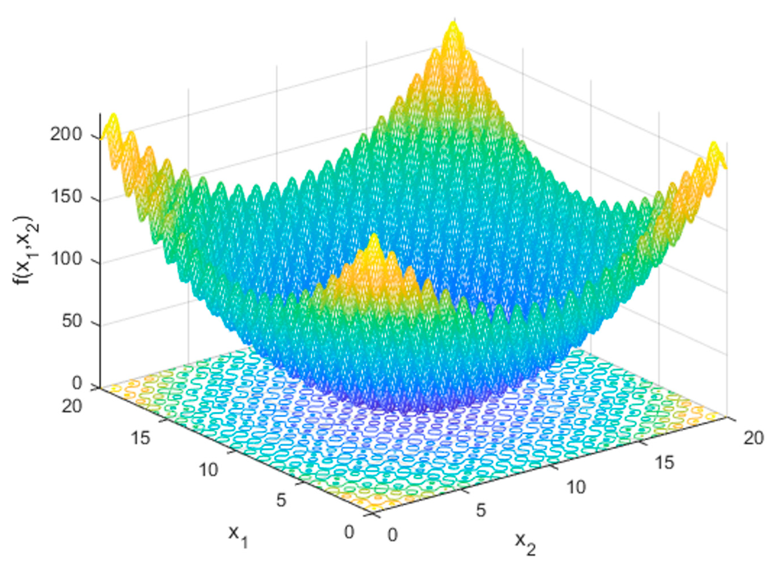
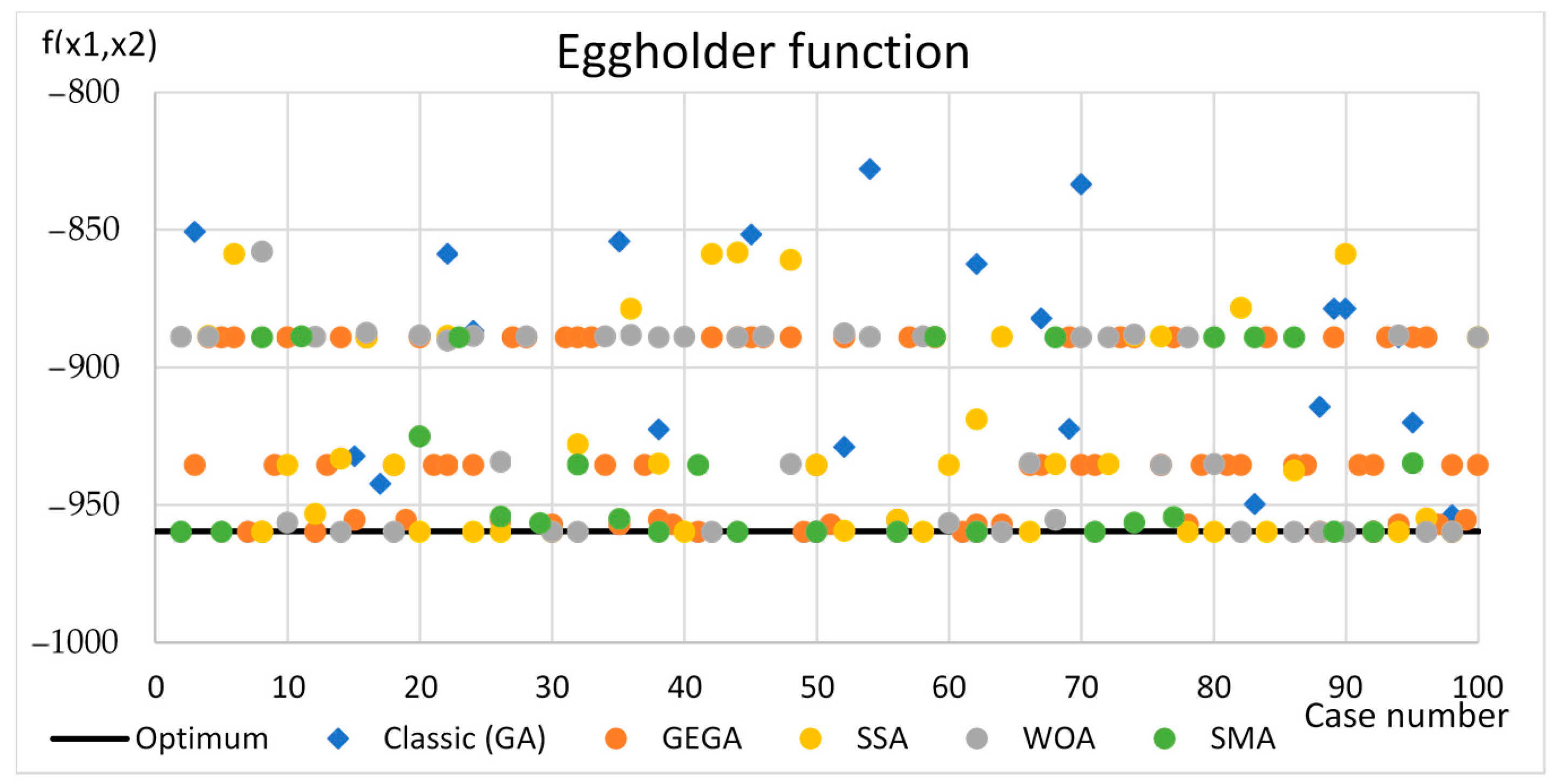
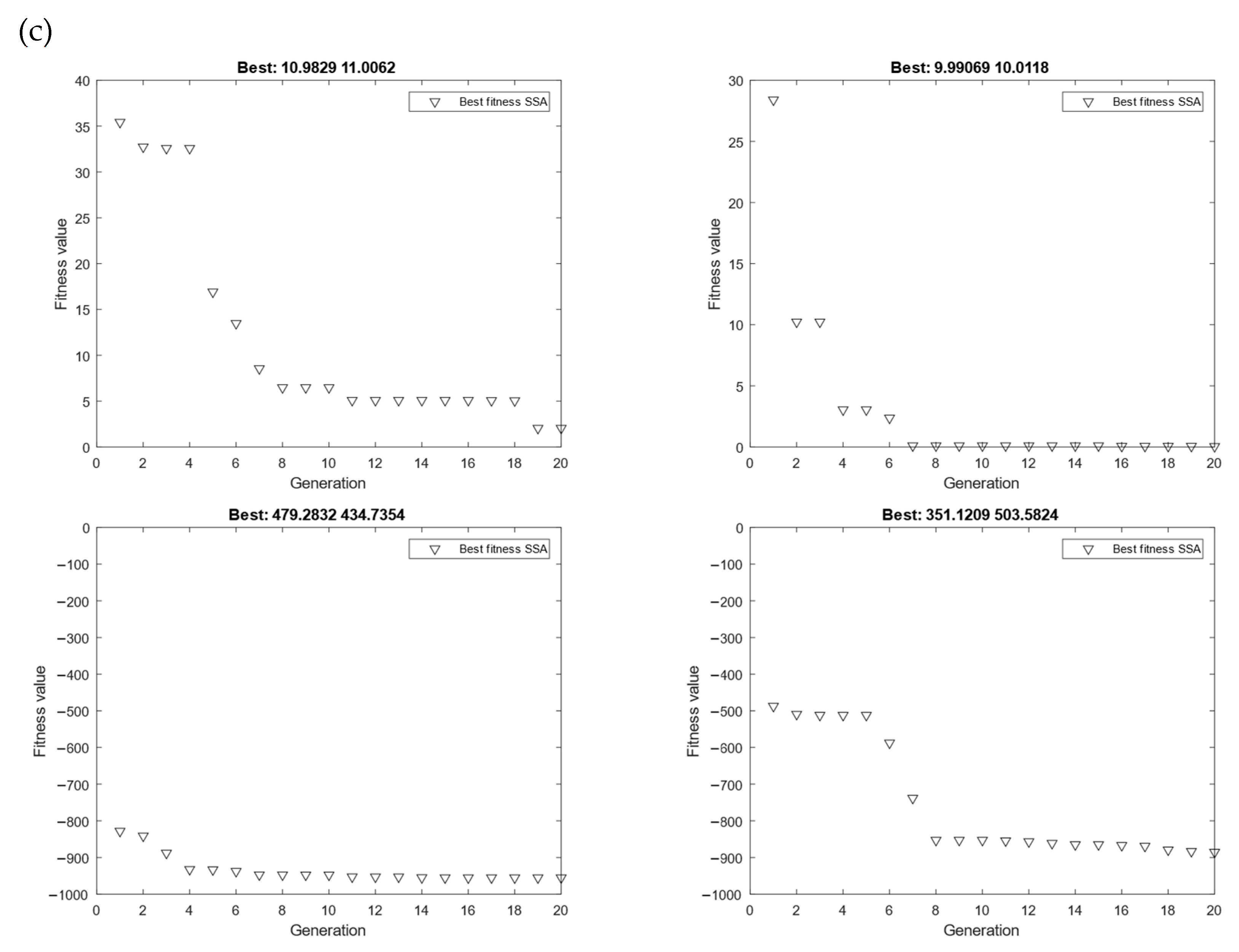
3.1. Testing Functions

The algorithm was examined on the basis of the Eggholder function minimum search [62], (Figure 1, Figure 2) and a modified one, by shifting the minimum from point (0.0) to point (10.10) of the Rastrigin function [63], (Figure 3):

$$f\left(x\right)=-\left(x_2+47\right)sin\sqrt{\left|\frac{x_1}{2}+x_2+47\right|}-x_{1}sin\sqrt{\left|x_1-\left(x_2+47\right)\right|}$$

(1)

$$f\left(x\right)=20+{\left(x_1-10\right)}^2+{\left(x_2-10\right)}^2+-10\left[cos\left(2\pi \left(x_1-10\right)\right)+cos\left(2\pi \left(x_2-10\right)\right)\right]$$

(2)

It was noticed that the suggested algorithm indicated values not of the global minimum, but occurring around this minimum. The gradient algorithm (“fmincon”, interior-point method) was employed to determine the global minimum, following the last program iteration.

The genetic algorithm without modification (“ga” function in MATLAB) was used for validation, but with a constraint on the population size and total number of generations, consistent with the number of generations and the population size of the modified algorithm (10 individuals in the population, 20 generations).

The proprietary GEGA was employed to optimize the Eggholder function. The GAGE algorithm code was compiled in the MATLAB language. The code was listed as in Appendix A and Appendix B. All the following calculations were performed on a computer with the following specifications: Intel(R) Xeon(R) W-1370P @ 3.60 GHz, 64 GB RAM.

The pseudocode of GEGA Algorithm 1 is presented below:

Algorithm 1:
Input:	“initial population”(one agent), “global lower boundary conditions (BC)”, “global upper BC”, “initial agent”, “number of iteration”
“best agent” “initial population” For all “number of iteration” Do:   If MOD(“number of iteration”,3) = 0 or “number of iteration” = 1     Lower local BC ← global lower BC     Upper local BC ← global upper BC   Else     Lower local BC ← 20% of global lower BC (around last “best agent”)     Upper local BC ← 20% of global upper BC (around last “best agent”)   End If     Until “number of generation” < 2     “number of generation” ← “number of generation”+1     Do: “Genetic Algorithm” → update “population”   End Until     “population” ← Sort “population”   “best agent” ← best of “population”   Delete “population” except 3 best and 3 worst agents   “initial population” ← “population”   End For Found minimum by “gradient method”, start from “best agent”

3.2. Algorithm Validation

Figure 4 and Figure 5 present convergence tests for the classic algorithm and modified algorithm, starting from the same initial population. The results are presented on the basis of the Eggholder function optimization.

The modified algorithm [63] reaches the global minimum region, while the classic algorithm, in the vast majority of cases, reaches one of the local minimums, and is unable to go beyond it. As for the GEGA, a seemingly chaotic convergence change in relation to the mean value can be noted. This change is also “chaotic” as far as the best-fit value is concerned; however, it improves steadily. The considerable difference between the best-fit value and the mean value results from the behavior of the three worst-fit individuals in the population. This makes it possible to extend the population gene pool and facilitates going beyond the local minimum.

A total of 100 attempts to search for Eggholder and Rastrigin function minimum were made. Optimization results for the Eggholder are presented in Figure 6, and such results for the Rastrigin function are presented in Figure 7. The examination included optimal solutions indicated by the classic algorithm (GA) (highlighted blue) and solutions indicated by the modified GEGA (highlighted orange), while the real global minimum of the objective function is marked with a grey line.

It can be observed that, unlike the classic algorithm, the modified algorithm is able to find the global minimum, with a small number of objective function value calculations. The modified GEGA moreover indicates clearly deeper local minimums than the classic algorithm. Both for the Eggholder function and Rastrigin function, almost all optimization results were better than the best results achieved with the classic algorithm, starting from the same initial population. The classic algorithm appears to be more effective than the modified algorithm only for 17 initial populations for the Eggholder function and one population for the Rastrigin function. The results were also compared with other contemporary algorithms such as Whale Optimization Algorithm (WOA) [64], Slime Mould Algorithm (SMA) [65], and Sparrow Search Algorithm (SSA) [66], as shown in

Table 1. Comparison of results of optimization of classic GA, GEGA, WOA, SMA, and SSA algorithms for Eggholder and Rastrigin functions.

Function	Point and Value of Minimum of the Function		Arithmetic Mean
			Classic GA	GEGA	WOA	SSA	SMA
Rastrigin	$x_1$	10	9.96	9.98	9.72	9.95	9.85
	$x_2$	10	10.10	10.04	9.90	10.02	9.71
	$f\left(x_1,x_2\right)$	0	7.65	0.24	5.69	1.77	1.44
Eggholder	$x_1$	512	356	387	407	429	427
	$x_2$	404.2319	343	405	432	406	411
	$f\left(x_1,x_2\right)$	−959.6407	−610	−833	−876	−870	−872
Function	Point and value of minimum of the function		Standard deviation
			Classic GA	GEGA	WOA	SSA	SMA
Rastrigin	$x_1$	1.63	1.63	0.34	1.47	0.88	0.97
	$x_2$	1.85	1.85	0.34	1.59	0.90	0.91
	$f\left(x_1,x_2\right)$	7.17	7.17	0.47	4.94	1.59	2.70
Eggholder	$x_1$	131	131	97	103	95	99
	$x_2$	132	132	110	97	106	104
	$f\left(x_1,x_2\right)$	183	183	163	129	141	141

as well as Figure 6 and Figure 7.

For both the Eggholder function and the Rastrigin function, the results are clearly distributed in two bands, with the band for the results of the GEGA clearly narrower and closer to the line of the global minimum of the function than for the GA. This is evidenced by the smaller value of the standard deviation and the smaller value of the arithmetic mean. It should be noted, however, that the suggested GEGA initially indicates the area where the global minimum is suspected, and then uses the gradient algorithm to indicate local minima. The final optimization in the GEGA using gradient methods was not included in the count of the total calculated number of solutions. The number of iterations used to determine the final minimum of the “fmincon” function ranged from one to two. The use of gradient methods for the classical algorithm did not affect the determined minimum.

In Figure 8, the convergence for the WOA, SSA, and SMA algorithms was presented.

Compared to the other algorithms, for the Rastrigin function, the GEGA has the smallest standard deviation and the highest accuracy in finding the global minimum. For Eggholder functions, all tested algorithms have similar accuracy and uncertainty of solutions. This may be due to the fact that GEGA uses a variable, instantaneous solution space, which allows it to track trends in changes in the local minima of the function.

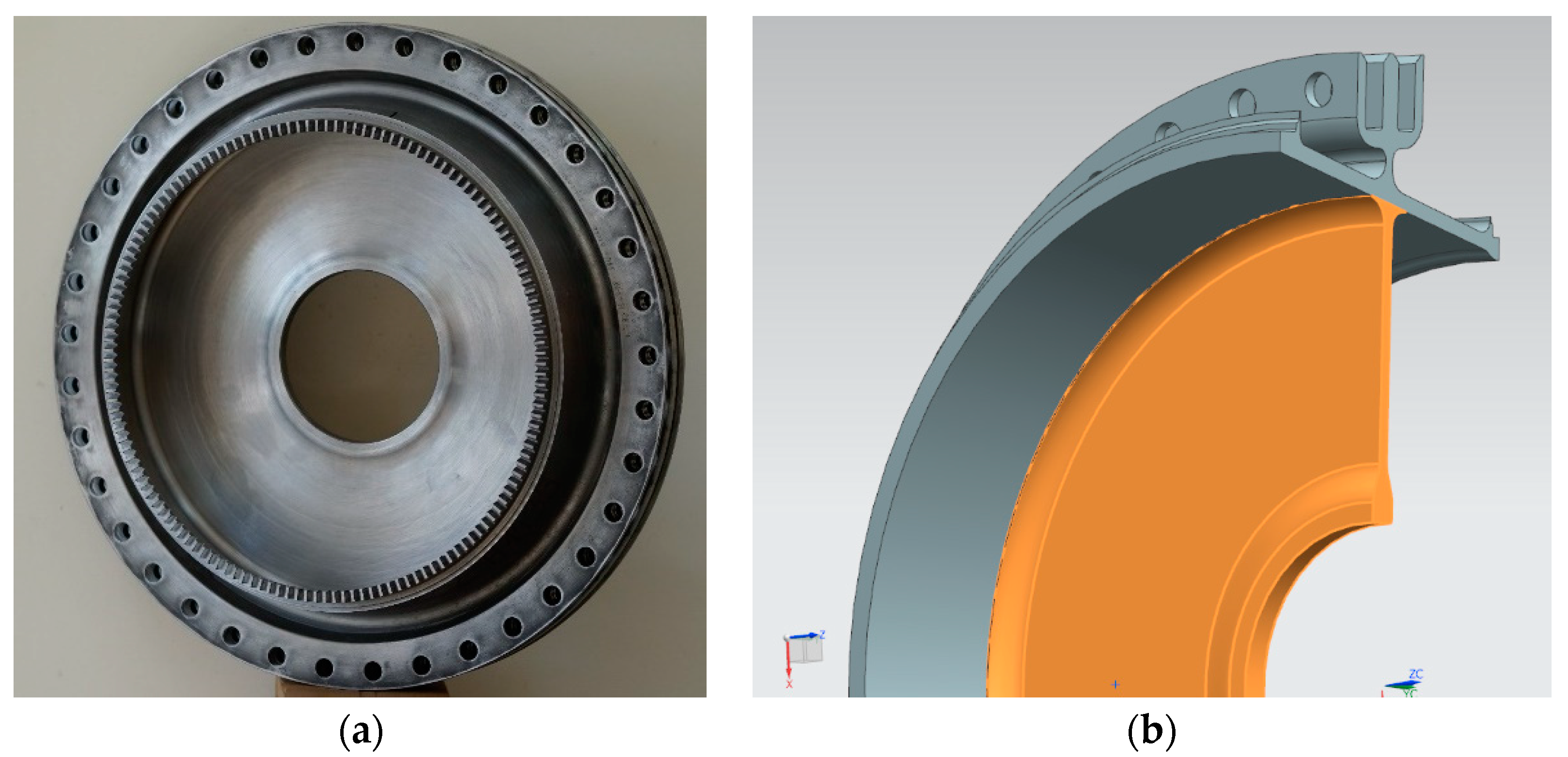
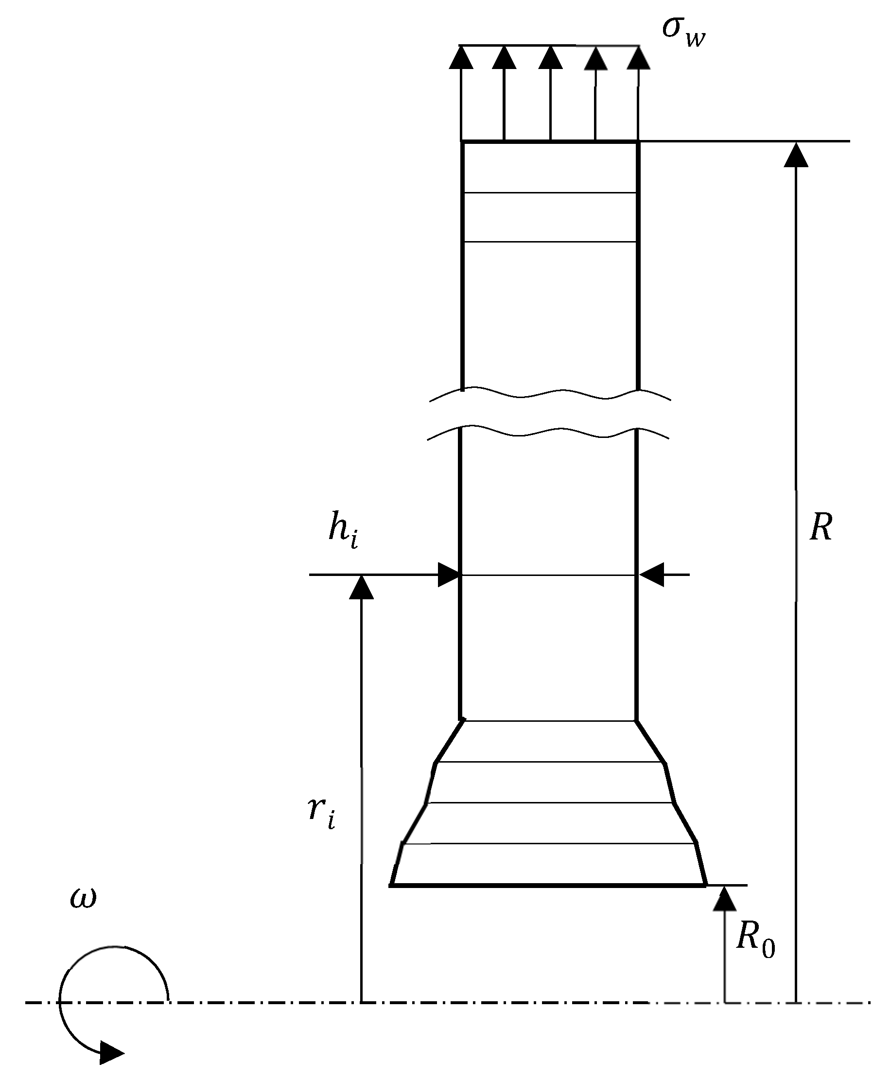
4. Compressor Disc Optimization

Using the previously presented algorithm, an optimization process was carried out (the part of the shield marked in orange in Figure 9). The optimization of such a design layout made it possible to analyze the validity and correctness of the modified genetic algorithm.

Model and analysis were based on a previous paper [25], where FEM was used to calculate stress (von Mises) distribution in the nodes of the disc. The disc was divided into eighteen finite elements. The elements were 1D with linearly variable thickness. The FEM algorithm was created by the authors and validated in paper [25]. In Figure 10, a simplified model of the disc was presented.

The classic GA and GEGA were comprised. For both algorithms were added boundary conditions to prevent increasing the thickness of the disk for the i + 1 node relative to the i-th node. The GA was default by MATLAB. Aim function was mass minimization, assuming that the allowable stresses (von Mises) are not exceeded. This condition was taken into account by means of a penalty function, the value of which depended on the difference between von Mises and allowable stresses.

For GE and GEGA, starting from the same starting point, 10 optimization processes were carried out. On this basis, the mean running time of the algorithms, as well as the mean and minimum weight after optimization, were estimated.

In

Table 2. Comparison of results of optimization of classic GA and GEGA for FEM analysis, where Δ is MAE based on GA.

	GA	GEGA	Δ [%]
Time (s)	40.30	5.67	85.94
Medium Mass (kg)	1.062	1.066	−0.301
Minimum Mass (kg)	1.058	1.059	−0.057

and Figure 11, time of optimization and mass were compared.

In Figure 12, Figure 13, Figure 14, Figure 15 and Figure 16, for ten cycles of optimization by GA and GEGA, thickness ($h$) and von Misese stresses distribution ($\sigma$) for mesh nodes was presented.

In Figure 15, for GA and GEGA optimization, mean value thickness ($h$) and von Mises stresses ($\sigma$) distribution was presented.

The results presented in Figure 15 are consistent. Only for fifth node are small differences for thickness in favor of the GA. However, differences in time of optimization (Figure 11) confirm the legitimacy of using the GEGA.

In paper [47], the ANN surrogate model and the GA were presented and time of optimization of the example above problem (Figure 9) was reduced by approximately 40% by the ANN surrogate model. Our new modification reduced the time of optimization by nearly 86%.

5. Conclusions

It can therefore be concluded that the suggested genetic algorithm modification is effective and, in addition, simple to implement. The mean value of the minimum indicated by the suggested GEGA was −833 and 0.24 for the Rastrigin function (minimum equal to −959) and Eggholder function (minimum equal to 0), where, for the classic algorithm, mean values amounted to −610 and 7.65, respectively. Moreover, the GEGA was able to find the global minimum for the Eggholder function with an accuracy of up to 9.5 (i.e., 0.01 of the global extrema value), in 22 of the 100 optimization attempts; for the Rastrigin function, it was achieved with an accuracy of up to 0.01, in 78 of the 100 attempts. With the same number of iterations, the classic algorithm only once found the global minimum for the Eggholder function, with the preset accuracy.

The suggested Great Extinctions Genetic Algorithm can be applied wherever the minimization of the number of objective function value calculations (or penalty function) is an important factor due to their high cost or time-consuming nature. As shown in Section 4, the GEGA performs similarly or better than the other algorithms tested for a small population (10 agents) and iterations (20). For 100 Eggholder function optimizations, the GEGA performs slightly worse on average than the WOA, SMA, or SSA algorithms. However, for the Rastrigin function, only the GEGA can find the minimum of the objective function almost every time for a small population and number of iterations.

5.1. Limitations

Whenever minimizing the number of samplings of the objective function is not important, a better option is to use another of the compared algorithms. Similarly, if it is expected that the objective function has no trend, the GEGA is also not better than other compared algorithms.

5.2. Further Research

Further work on algorithm development will therefore focus on optimizing its parameters, such as population size, large extinction event frequency, or size of the instantaneous space of the admissible solutions. There will also be comparative analyses of the proposed algorithm with algorithms using a surrogate model determined based on neural networks. However, it can already be assumed that the SSN surrogate model will require significantly more samples of the objective function. In addition, when analyzing the results of the studies presented in Section 3, it is worth considering the use of a variable solution space in other compared algorithms.

In the process of using genetic algorithms, artificial neural networks, additional emphasis is placed on making sure that the artificial neural network is not deceived by an artificial or real example of adversity and that there is no built-in algorithm bias. In the case of strength analysis, particularly relevant here are the errors of the FEM model in the case of parametric generated samples of the objective function. Hence, verifying large sets generates the additional problem that neural networks usually require significant amounts of data, e.g., supervised data, which may not always be available for a given problem, especially for edge cases. In fact, most genetic algorithms and large neural networks will have trouble properly starting the optimization process if the input dataset is not large and diverse enough. As opposed to neural networks and the classical GA, the proposed algorithm does not require a high number of samples to work properly. Moreover, large amounts of input data are computationally expensive to train and industrialize; hence, the natural combination of genetic algorithms and artificial neural networks is strongly justified.

References

1. Chen, L.; Asteris, P.G.; Tsoukalas, M.Z.; Armaghani, D.J.; Ulrikh, D.V.; Yari, M. Forecast of Airblast Vibrations Induced by Blasting Using Support Vector Regression Optimized by the Grasshopper Optimization (SVR-GO) Technique. Appl. Sci. 2022, 12, 9805. [Google Scholar] [CrossRef]
2. Li, G.; Li, Y.; Chen, H.; Deng, W. Fractional-Order Controller for Course-Keeping of Underactuated Surface Vessels Based on Frequency Domain Specification and Improved Particle Swarm Optimization Algorithm. Appl. Sci. 2022, 12, 3139. [Google Scholar] [CrossRef]
3. Szalai, S.; Herold, B.; Kurhan, D.; Németh, A.; Sysyn, M.; Fischer, S. Optimization of 3D Printed Rapid Prototype Deep Drawing Tools for Automotive and Railway Sheet Material Testing. Infrastructures 2023, 8, 43. [Google Scholar] [CrossRef]
4. Ameen, F. Optimization of the Synthesis of Fungus-Mediated Bi-Metallic Ag-Cu Nanoparticles. Appl. Sci. 2022, 12, 1384. [Google Scholar] [CrossRef]
5. Dong, L.; Qin, L.; Xie, X.; Zhang, L.; Qin, X. Collaborative Optimization Method for Multi-Train Energy-Saving Control with Urban Rail Transit Based on DRLDA Algorithm. Appl. Sci. 2023, 13, 2454. [Google Scholar] [CrossRef]
6. Burrascano, P. Parameter Optimization for an Accurate Swept-Sine Identification Procedure of Nonlinear Systems. Appl. Sci. 2023, 13, 1223. [Google Scholar] [CrossRef]
7. Imran, M.; Shi, D.; Tong, L.; Waqas, H.M. Design optimization of composite submerged cylindrical pressure hull using genetic algorithm and finite element analysis. Ocean. Eng. 2019, 190, 106443. [Google Scholar] [CrossRef]
8. Chan, C.M.; Bai, H.L.; He, D.Q. Blade shape optimization of the Savonius wind turbine using a genetic algorithm. Appl. Energy 2018, 213, 148–157. [Google Scholar] [CrossRef]
9. Ding, Y.; Zhang, W.; Yu, L.; Lu, K. The accuracy and efficiency of GA and PSO optimization schemes on estimating reaction kinetic parameters of biomass pyrolysis. Energy 2019, 176, 582–588. [Google Scholar] [CrossRef]
10. Holland, J.H. Genetic Algorithms. Sci. Am. 1992, 267, 66–73. Available online: http://papers.cumincad.org/data/works/att/7e68.content.pdf (accessed on 24 August 2022). [CrossRef]
11. Lee, C.K.H. A review of applications of genetic algorithms in operations management. Eng. Appl. Artif. Intell. 2018, 76, 1–12. [Google Scholar] [CrossRef]
12. Katoch, S.; Chauhan, S.S.; Kumar, V. A review on genetic algorithm: Past, present, and future. Multimed. Tools Appl. 2021, 80, 8091–8126. [Google Scholar] [CrossRef] [PubMed]
13. Deb, K.; Agrawal, R.B. Simulated Binary Crossover for Continuous Search Space. Complex Syst. 1995, 9, 115–148. Available online: https://citeseerx.ist.psu.edu/viewdoc/download?doi=10.1.1.26.8485&rep=rep1&type=pdf (accessed on 8 August 2022).
14. Eshelman, L.J.; Caruana, R.A.; Schaffer, J.D. Biases in the Crossover Landscape. In Proceedings of the Third International Conference on Genetic Algorithms, 1989; pp. 10–19. Available online: https://www.academia.edu/17531298/Biases_in_the_Crossover_Landscape (accessed on 7 July 2022).
15. Michalewicz, Z. Genetic Algorithms + Data Structures = Evolution Programs; Springer: Berlin/Heidelberg, Germany, 1996. [Google Scholar] [CrossRef]
16. Ono, I.; Kita, H.; Kobayashi, S. A Real-coded Genetic Algorithm using the Unimodal Normal Distribution Crossover. In Advances in Evolutionary Computing; Springer: Berlin/Heidelberg, Germany, 2003; pp. 246–253. [Google Scholar] [CrossRef]
17. Deep, K.; Thakur, M. A new crossover operator for real coded genetic algorithms. Appl. Math. Comput. 2007, 188, 895–911. [Google Scholar] [CrossRef]
18. Blickle, T.; Thiele, L. A comparison of selection schemes used in evolutionary algorithms. Evol. Comput. 1996, 4, 361–394. [Google Scholar] [CrossRef]
19. Baker, J.E. Adaptive selection methods for genetic algorithms. In Proceedings of the An International Conference on Genetic Algorithms and Their Applications Pittsburg, Pittsburg, PA, USA, 24–26 July 1985; ISBN 0-8058-0426-9. [Google Scholar]
20. Goldberg, D.E.; Korb, B.; Drb, K. Messy genetic algorithms: Motivation, analysis, and first results. Complex Syst. 1989, 3, 493–530. [Google Scholar]
21. Dianati, M.; Song, I.; Treiber, M. An Introduction to Genetic Algorithms and Evolution Strategies; Technical Report; University of Waterloo: Waterloo, ON, Canada, 2002; Available online: https://citeseerx.ist.psu.edu/viewdoc/download?doi=10.1.1.92.6910&rep=rep1&type=pdf (accessed on 24 August 2022).
22. Sivaram, M.; Batri, K.; Mohammed, A.S.; Porkodi, V. Exploiting the Local Optima in Genetic Algorithm using Tabu Search. Indian J. Sci. Technol. 2019, 12, 1–13. [Google Scholar] [CrossRef]
23. Hamamoto, A.H.; Carvalho, L.F.; Sampaio, L.D.H.; Abrão, T.; Proença, M.L. Network Anomaly Detection System using Genetic Algorithm and Fuzzy Logic. Expert Syst. Appl. 2018, 92, 390–402. [Google Scholar] [CrossRef]
24. Reynolds, J.; Rezgui, Y.; Kwan, A.; Piriou, S. A zone-level, building energy optimisation combining an artificial neural network, a genetic algorithm, and model predictive control. Energy 2018, 151, 729–739. [Google Scholar] [CrossRef]
25. Kieszek, R.; Kozakiewicz, A.; Rogólski, R. Optimization of a Jet Engine Compressor Disc with Application of Artificial Neural Networks for Calculations Related to Time and Mass Criteria. Adv. Sci. Technol. Res. J. 2021, 15, 208–218. [Google Scholar] [CrossRef]
26. Jaworski, B.; Kuczkowski, L.; Śmierzchalski, R.; Kolendo, P. Extinction event concepts for the evolutionary algorithms. Przegląd Elektrotechniczny 2012, 88, 252–255. [Google Scholar]
27. Jafar-Zanjani, S.; Inampudi, S.; Mosallaei, H. Adaptive Genetic Algorithm for Optical Metasurfaces Design. Sci. Rep. 2018, 8, 1–16. [Google Scholar] [CrossRef]
28. Iba, K. Reactive power optimization by genetic algorithm. IEEE Trans. Power Syst. 1994, 9, 685–692. [Google Scholar] [CrossRef]
29. Ding, S.; Su, C.; Yu, J. An optimizing BP neural network algorithm based on genetic algorithm. Artif. Intell. Rev. 2011, 36, 153–162. [Google Scholar] [CrossRef]
30. Deaven, D.M.; Ho, K.M. Molecular Geometry Optimization with a Genetic Algorithm. Phys. Rev. Lett. 1995, 75, 288–291. [Google Scholar] [CrossRef]
31. Kim, C.; Batra, R.; Chen, L.; Tran, H.; Ramprasad, R. Polymer design using genetic algorithm and machine learning. Comput. Mater. Sci. 2021, 186, 110067. [Google Scholar] [CrossRef]
32. Kozakiewicz, A.; Kieszek, R. Artificial Neural Network Structure Optimisation in the Pareto Approach on the Example of Stress Prediction in the Disk-Drum Structure of an Axial Compressor. Materials 2022, 15, 4451. [Google Scholar] [CrossRef]
33. Ryu, J. A Visual Saliency-Based Neural Network Architecture for No-Reference Image Quality Assessment. Appl. Sci. 2022, 12, 9567. [Google Scholar] [CrossRef]
34. Liang, B.; Han, S.; Li, W.; Fu, D.; He, R.; Huang, G. Accurate Spatial Positioning of Target Based on the Fusion of Uncalibrated Image and GNSS. Remote. Sens. 2022, 14, 3877. [Google Scholar] [CrossRef]
35. Li, Z.; Wang, Y.; Zhang, N.; Zhang, Y.; Zhao, Z.; Xu, D.; Ben, G.; Gao, Y. Deep Learning-Based Object Detection Techniques for Remote Sensing Images: A Survey. Remote Sens. 2022, 14, 2385. [Google Scholar] [CrossRef]
36. Wang, B.; Wang, S.; Zeng, D.; Wang, M. Convolutional Neural Network-Based Radar Antenna Scanning Period Recognition. Electronics 2022, 11, 1383. [Google Scholar] [CrossRef]
37. Kim, K. Multi-Agent Deep Q Network to Enhance the Reinforcement Learning for Delayed Reward System. Appl. Sci. 2022, 12, 3520. [Google Scholar] [CrossRef]
38. Zhao, X.; Shao, F.; Zhang, Y. A Novel Joint Adversarial Domain Adaptation Method for Rotary Machine Fault Diagnosis under Different Working Conditions. Sensors 2022, 22, 9007. [Google Scholar] [CrossRef] [PubMed]
39. Kondo, K.; Hasegawa, T. Sensor-Based Human Activity Recognition Using Adaptive Class Hierarchy. Sensors 2021, 21, 7743. [Google Scholar] [CrossRef] [PubMed]
40. Daneshdoost, F.; Hajiaghaei-Keshteli, M.; Sahin, R.; Niroomand, S. Tabu search based hybrid meta-heuristic approaches for schedule-based production cost minimization problem for the case of cable manufacturing systems. Informatica 2022, 33, 499–522. [Google Scholar] [CrossRef]
41. Ghazikhani, A.; Babaeian, I.; Gheibi, M.; Hajiaghaei-Keshteli, M.; Fathollahi-Fard, A.M. A Sustainable Climate Forecast System for Post-Processing of Precipitation with Application of Machine Learning Computations. 2022. Available online: https://doi.org/10.21203/rs.3.rs-1552614/v1 (accessed on 11 March 2023). [CrossRef]
42. Ghazikhani, A.; Babaeian, I.; Gheibi, M.; Hajiaghaei-Keshteli, M.; Fathollahi-Fard, A.M. A Smart Post-Processing System for Forecasting the Climate Precipitation Based on Machine Learning Computations. Sustainability 2022, 14, 6624. [Google Scholar] [CrossRef]
43. Abdi, A.; Abdi, A.; Akbarpour, N.; Amiri, A.S.; Hajiaghaei-Keshteli, M. Innovative approaches to design and address green supply chain network with simultaneous pick-up and split delivery. J. Clean. Prod. 2020, 250, 119437. [Google Scholar] [CrossRef]
44. Liao, Y.; Kaviyani-Charati, M.; Hajiaghaei-Keshteli, M.; Diabat, A. Designing a closed-loop supply chain network for citrus fruits crates considering environmental and economic issues. J. Manuf. Syst. 2020, 55, 199–220. [Google Scholar] [CrossRef]
45. Cheraghalipour, A.; Paydar, M.M.; Hajiaghaei-Keshteli, M. An integrated approach for collection center selection in reverse logistics. Int. J. Eng. 2017, 30, 1005–1016. [Google Scholar]
46. Taghipour, A.; Khazaei, M.; Azar, A.; Ghatari, A.R.; Hajiaghaei-Keshteli, M.; Ramezani, M. Creating Shared Value and Strategic Corporate Social Responsibility through Outsourcing within Supply Chain Management. Sustainability 2022, 14, 1940. [Google Scholar] [CrossRef]
47. Chouhan, V.K.; Khan, S.H.; Hajiaghaei-Keshteli, M. Sustainable planning and decision-making model for sugarcane mills considering environmental issues. J. Environ. Manag. 2021, 303, 114252. [Google Scholar] [CrossRef] [PubMed]
48. Tang, Y.; Tan, S.; Zhou, D. An Improved Failure Mode and Effects Analysis Method Using Belief Jensen–Shannon Divergence and Entropy Measure in the Evidence Theory. Arab. J. Sci. Eng. 2023, 48, 7163–7176. [Google Scholar] [CrossRef]
49. Fathollahi-Fard, A.M.; Hajiaghaei-Keshteli, M.; Tavakkoli-Moghaddam, R. Red deer algorithm (RDA): A new nature-inspired meta-heuristic. Soft Comput. 2020, 24, 14637–14665. [Google Scholar] [CrossRef]
50. Chouhan, V.K.; Khan, S.H.; Hajiaghaei-Keshteli, M. Metaheuristic approaches to design and address multi-echelon sugarcane closed-loop supply chain network. Soft Comput 2021, 25, 11377–11404. [Google Scholar] [CrossRef]
51. Fathollahi-Fard, A.M.; Hajiaghaei-Keshteli, M.; Tavakkoli-Moghaddam, R. The social engineering optimizer (SEO). Eng. Appl. Artif. Intell. 2018, 72, 267–293. [Google Scholar] [CrossRef]
52. Goodarzian, F.; Ghasemi, P.; Kumar, V.; Abraham, A. A new modified social engineering optimizer algorithm for engineering applications. Soft Comput. 2022, 26, 4333–4361. [Google Scholar] [CrossRef]
53. Piskin, A.; Baklacioglu, T.; Turan, O. Optimization and off-design calculations of a turbojet engine using the hybrid ant colony—Particle swarm optimization method. Aircr. Eng. Aerosp. Technol. 2022, 94, 1025–1035. [Google Scholar] [CrossRef]
54. Aydın, E.; Turan, O. Performance models of passenger aircraft and propulsion systems based on particle swarm and Spotted Hyena Optimization methods. Energy 2023, 268, 126659. [Google Scholar] [CrossRef]
55. Hajiaghaei-Keshteli, M.; Aminnayeri, M. Keshtel Algorithm (KA); a new optimization algorithm inspired by Keshtels’ feeding. In Proceedings of the IEEE Conference on Industrial Engineering and Management Systems, Bangkok, Thailand, 10–13 December 2013; pp. 2249–2253. [Google Scholar]
56. Hajiaghaei-Keshteli, M.; Aminnayeri, M. Solving the integrated scheduling of production and rail transportation problem by Keshtel algorithm. Appl. Soft Comput. 2014, 25, 184–203. [Google Scholar] [CrossRef]
57. Chouhan, V.K.; Khan, S.H.; Hajiaghaei-Keshteli, M. Hierarchical tri-level optimization model for effective use of by-products in a sugarcane supply chain network. Appl. Soft Comput. 2022, 128, 109468. [Google Scholar] [CrossRef]
58. Salehi-Amiri, A.; Zahedi, A.; Gholian-Jouybari, F.; Calvo, E.Z.R.; Hajiaghaei-Keshteli, M. Designing a Closed-loop Supply Chain Network Considering Social Factors; A Case Study on Avocado Industry. Appl. Math. Model. 2021, 101, 600–631. [Google Scholar] [CrossRef]
59. Abbasi, S.; Daneshmand-Mehr, M.; Kanafi, A.G. Green Closed-Loop Supply Chain Network Design During the Coronavirus (COVID-19) Pandemic: A Case Study in the Iranian Automotive Industry. Environ. Model. Assess. 2022, 28, 69–103. [Google Scholar] [CrossRef]
60. Lehman, J.; Miikkulainen, R. Extinction Events Can Accelerate Evolution. PLoS ONE 2015, 10, e0132886. [Google Scholar] [CrossRef]
61. Och, L.M.; Shields-Zhou, G.A. The Neoproterozoic oxygenation event: Environmental perturbations and biogeochemical cycling. Earth-Science Rev. 2012, 110, 26–57. [Google Scholar] [CrossRef]
62. Rastrigin, L.A. Systems of Extremal Control; Nauka: Moscow, Russia, 1974. [Google Scholar]
63. Available online: https://github.com/RafalKieszek/GEGA (accessed on 28 November 2022).
64. Chakraborty, S.; Saha, A.K.; Sharma, S.; Mirjalili, S.; Chakraborty, R. A novel enhanced whale optimization algorithm for global optimization. Comput. Ind. Eng. 2021, 153, 107086. [Google Scholar] [CrossRef]
65. Wu, X.; Wang, Z. Multi-objective optimal allocation of regional water resources based on slime mould algorithm. J. Supercomput. 2022, 78, 18288–18317. [Google Scholar] [CrossRef]
66. Gad, A.G.; Sallam, K.M.; Chakrabortty, R.K.; Ryan, M.J.; Abohany, A.A. An improved binary sparrow search algorithm for feature selection in data classification. Neural Comput. Appl. 2022, 34, 15705–15752. [Google Scholar] [CrossRef]
Figure 1. Eggholder function. f m i n = f ( 512 ; 404.23 ) = 959.64 .
Applsci 13 05584 g001
Figure 2. Eggholder function level lines with the global minimum highlighted in red.
Applsci 13 05584 g002
Figure 3. Modify Rastrigin function. f m i n = f ( 10 , 10 ) = 0 .
Applsci 13 05584 g003
Figure 4. Convergence for the classic genetic algorithm.
Applsci 13 05584 g004
Figure 5. Convergence for the modified Great Extinction Genetic Algorithm (GEGA).
Applsci 13 05584 g005
Figure 6. Results of optimization of Eggholder function for Genetic Algorithm (GA), Great Extinction Genetic Algorithm (GEGA), Whale Optimization Algorithm (WOA), Slime Mould Algorithm (SMA), and Sparrow Search Algorithm (SSA).
Applsci 13 05584 g006
Figure 7. Results of optimization of Rastrigin function for Genetic Algorithm (GA), Great Extinction Genetic Algorithm (GEGA), Whale Optimization Algorithm (WOA), Slime Mould Algorithm (SMA), and Sparrow Search Algorithm (SSA). A total of 27 points for the minimum greater than 10 for the classical algorithm were ignored.
Applsci 13 05584 g007
Figure 8. Convergence for the WOA (a), SSA, (b) and SMA (c) algorithms.
Applsci 13 05584 g008aApplsci 13 05584 g008b
Figure 9. The disk of the axial compressor stage of a turbine jet engine: the real object (a) and the reference model of the disc with the optimized area marked (b).
Applsci 13 05584 g009
Figure 10. Model of profiled disc with computational mesh density shown, where ω —angular velocity, R 0 —radius of the central hole, R —outer radius of the disc, σ w —rim drawing, r i —radial coordinate of the i-th design node, h i —thickness of the i-th node.
Applsci 13 05584 g010
Figure 11. Mean time of optimization and mean and minimal mass for GE and GEGA: real value (a) and relative value (b), where GA results are the basis.
Applsci 13 05584 g011
Figure 12. Distribution of thickness ( h ) for nodes ( n ) for GA optimization for ten series.
Applsci 13 05584 g012
Figure 13. Distribution of von Mises stresses ( σ ) for nodes ( n ) for GA optimization for ten series.
Applsci 13 05584 g013
Figure 14. Distribution of thickness ( h ) for nodes ( n ) for GEGA optimization for ten series.
Applsci 13 05584 g014
Figure 15. Distribution of von Mises stresses ( σ ) for nodes ( n ) for GEGA optimization for ten series.
Applsci 13 05584 g015
Figure 16. Mean value thickness ( h ) and von Mises stresses ( σ ) distribution for GA and GEGAs.
Applsci 13 05584 g016