A Novel Active Noise Control Method Based on Variational Mode Decomposition and Gradient Boosting Decision Tree

Abstract

Diversified noise sources pose great challenges in the engineering of an ANC (active noise control) system design. To solve this problem, this paper proposes an ANC method based on VMD (variational mode decomposition) and Ensemble Learning. VMD is used to extract IMFs (Intrinsic Model Functions) of different types of noise and obtain the approximate entropy of each IMF. Clustering analysis on the output of VMD is conducted based on the PCA (principal component analysis) dimension reduction method and k-means++ method to get classification results for different noises. On the basis of the clustering results, different GBDT (gradient boosting decision tree) regressors are constructed for different noise types, in order to create a high-performance ANC system for multiple noise sources. To verify the effectiveness of the proposed method, this paper designed four simulation schemes for the ANC: obstacle-free rectangular enclosed space, rectangular enclosed space with obstacle, obstacle-free trapezoidal enclosed space and trapezoidal enclosed space with obstacle. When machine gun noise is used as an example, noise attenuation by the proposed method in four simulation schemes is −23.27 dB, −21.6 dB, −19.08 dB and −15.48 dB respectively.

1. Introduction

Active noise control (ANC) is a technology used to reduce noise in the target area by actively generating a sound field with an external sound source and overlaying the existing noise sound field. ANC technology takes the noise signal as input and adjusts the controller, to generate a secondary noise signal, thereby achieving noise control. However, when the noise signal changes with time and the noise type can not be predicted in advance, it difficult to track the noise in real time. The noise type in a real environment is usually unknown; therefore, multiple groups of control filter banks should be designed in an ANC system to achieve the noise suppression effect with higher precision. This study paper attempted to solve these two problems using feature extraction and regression algorithm with ensemble learning.

Variational mode decomposition (VMD), proposed by Dragomiretskiy in 2014 [1], is an adaptive and completely non-recursive mode variation signal processing method. VMD decomposes the signal into several signals of different frequency scales. VMD can determine the number of modes decomposed from the signal based on the actual situation, adaptively match the best central frequency and finite bandwidth of each mode in the search and solution process and achieve the effective separation and frequency domain division of the intrinsic mode components in the signal. Recently, VMD has been widely used in noise feature extraction. Li combined VMD with k-nearest neighbor mutual information to extract features of ship-radiated noise [2]. Yang proposed a secondary decomposition de-noising method for underwater acoustic signals with VMD [3]. Zhang applied VMD to obtain the noise intensity in intrinsic mode functions (IMFs) [4]. Wu applied the mini-batch multivariate VMD to achieve the de-noising of random seismic noise [5]. Wu and Zhang proposed a new method using VMD and a convolutional neural network to attenuate the white noise of a seismic trace [6]. Wei conducted a comparative investigation of VMD and empirical mode decomposition for the noise reduction of transient electromagnetic signals. The research suggests that VMD is expected to be used for signal interference suppression in the field of transient electromagnetic detection in the future [7].

Ensemble learning is a growing topic of interest in the field of pattern recognition and machine learning. It has attracted great attention, as it can significantly improve the accuracy and generalizability of learning systems [8,9]. In general, ensemble learning is divided into bagging, boosting and stacking and each of these three stages use algorithm designs based on the tree model. Advantages of a random forest are mainly reflected in two characteristics: It can process high-dimensional feature data without feature extraction [10,11] (the importance of each feature would be evident after training) and it is conducive to fast speed parallel computation. Therefore, this paper reports on designs of an ANC system based on an ensemble learning algorithm of random forest. Bagging ensemble learning algorithms attain the optimal prediction model by training multiple classifiers in parallel and then taking the average value [12,13]. The influence of the number of trees on prediction precision, however, should be taken into consideration when designing the bagging method. In theory, the effect should improve with an increase in the number of trees. The number of trees would not, however, affect the prediction precision greatly when it reaches a certain level. Stacking ensemble learning algorithms improve the prediction precision of the classifier by stacking individual learners together, but they are not suitable for online running due to their long computation time. In comparison with bagging and stacking ensemble learning algorithms, a boosting ensemble learning algorithm has a lower computation cost and higher prediction precision [14,15]. Therefore, a boosting ensemble learning method was adopted in this paper for the design of an ANC system.

Common boosting ensemble algorithms include adaptive boosting machine (AdaBM), gradient boosting decision tree (GBDT) [16], histogram-based gradient boosting machine (Hist-GBM) [17] and light gradient boosting machine (Light-GBM) [18]. Among these, GBM optimizes the loss function in the direction of the fastest gradient decline through orderly iteration. The Hist-GBM and Light-GBM algorithms are derived from GBDT. GBDT is widely used because it is easy to achieve high regression accuracy and generalizability. The GBDT is a decision tree with the introduction of two ideas, gradual lifting and shrink, which improve the generalizability of ordinary decision trees. The core point of GBDT is the accumulation of the predicted values from multiple decision trees, with the residual as the learning goal of each decision tree. Through the above analysis and discussion, this paper uses GBDT to design an ANC method for different noise types. Lu predicted airfoil self-noise using a GBDT with random forest [19]. Li proposed a new GBDT algorithm based on a Kalman filter to tackle time series prediction problems [20]. Based on GBDT and principal component analysis, Wu proposed a novel seismic trace interpolation method for irregularly sampled spatial data [21].

To address situations where the noise type is unknown, this paper designed an ANC based on VMD and GBDT algorithms with high real-time performance. To identify noise type automatically, a PCA dimensionality reduction algorithm and VMD algorithm were used to extract characteristics of input noise, in order to reduce data size. Then, a k-means clustering algorithm was applied to classify the extracted noise characteristics. Finally, GBDT regressors were constructed for different types of noise, to acheive the objective of an ANC system with high real-time performance and better noise reduction.

The rest of this paper is organized as follows: Section 2 presents the noise feature extraction based on VMD, noise type clustering based on PCA and k-meas++ and the ANC method based on GBDT. Section 3 illustrates the pre-processing of a noise dataset and numerical simulation of the ANC. Section 4 presents the results of analyses. The paper’s conclusions are in Section 5.

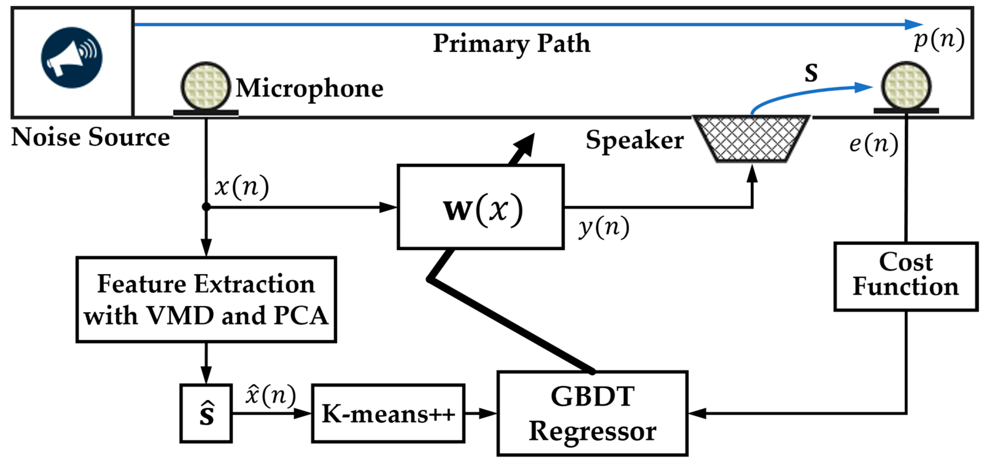
2. ANC Method Based on VMD and GBDT

2.1. Preliminaries

The schematic diagram of the proposed ANC method based on VMD and integrated learning algorithm is shown in Figure 1. The proposed ANC method includes an active noise control module, feature extraction module and gradient boosting decision tree module.

The ANC is a modular feedback control system, where $x\left(n\right)$ represents the reference signal, $y\left(n\right)$ represents the secondary path output (control output), $p\left(n\right)$ represents the primary noise, $e\left(n)=p\left(n\right)-y(n\right)$ represents the error signal, $s=\left[s_0, s_1, \cdots , s_{M-1}\right]$ represents the secondary path. In this model $\widehat{s}$ represents the estimated secondary path, and generally $\widehat{s}=s$. $w\left(n\right)={\left[w_0\left(n\right), w_1\left(n\right), \cdots , w_{N-1}\left(n\right)\right]}^{\mathrm{T}}$ represents the adaptive controller.

The feature extraction module includes two parts: a noise feature extraction based on VMD and noise clustering analysis based on PCA and k-means++. The module extracts the IMFs of noise data through VMD and gets the AE for each IMF of noise. The VMD processing result is taken as the input for the PCA and k-means to classify the noises. On the basis of the feature extraction and cluster analysis of noise data, the GBDT module generates different GBDT regressors for different noises, thereby creating an ANC for noise of different types.

2.2. Feature Extraction with VMD

The variational mode decomposition (VMD) decomposes the noise data $x\left(i\right)$ into intrinsic mode functions (IMFs) $u_k\left(i\right)$ with the number of $K$ [1]:

$$x\left(i\right)={\displaystyle \sum }_{k=1}^K{u}_k\left(i\right)=A_k\left(i\right)\cos \left[{\varphi }_k\left(i\right)\right]$$

(1)

where $K=6$ in this paper, ${\varphi }_k\left(i\right)$ is mode phase and $A_k\left(i\right)$ is the envelope. To obtain the IMFs and central frequency, the optimum of the augmented Lagrangian is performed as following:

$$\begin{gathered} L\left(u_k\left(t\right), f_k, {\lambda }_t\right)=\alpha {\displaystyle \sum }_{k=1}^K{\Vert \frac{d}{dt}\left[\left(\delta \left(t\right)+\frac{j}{\pi t}\right)\ast u_k\left(t\right)\right]e^{-j2\pi f_{k}t}\Vert }_2^2 \\ +{\Vert x\left(t\right)-{\displaystyle \sum }_{k=1}^K{u}_k\left(t\right)\Vert }_2^2+\langle {\lambda }_t, x_t-{\displaystyle \sum }_{k=1}^K{u}_k\left(t\right)\rangle \end{gathered}$$

(2)

where ${\lambda }_t$ is the Lagrangian coefficient, $\alpha$ is the scale factor, $\delta$ is the Fermi–Dirac distribution, ${\Vert ·\Vert }_2^2$ is the 2-norm and $\langle ·\rangle$ is the inner product. The VMD method captures the mode waveforms and central frequencies of the raw rolling bearing vibration signal in the frequency domain.

Furthermore, the approximate entropy (AE) [22] is used to transform the IMF sequences into six feature values for each noise dataset. A window with length of m was set for the noise convolution signals $X_c\left(1\right), X_c\left(2\right), \dots , X_c\left(N\right)$ with length of N. A set of vectors with dimension of m was thus obtained:

$$X_c\left(i\right)=\left\{X_c\left(i\right), X_c\left(i+1\right),\dots , X_c\left(i+m-1\right)\right\}, i=1, 2, \dots , N-m+1.$$

(3)

The distance between $X_c\left(i\right) \mathrm{and} X_c\left(j\right)$ is defined as the largest difference between the two corresponding elements and is calculated as:

$$d\left[X_c\left(i\right), X_c\left(j\right)\right]=\underset{k=0~m-1}{\max }\left[\left|X_c\left(i+k\right)-X_c\left(j+k\right)\right|\right].$$

(4)

$C_i^m\left(r\right)$, the ratio of $\left\{d\left[X_c\left(i\right), X_c\left(j\right)\right]<r\right\}$ to the total number of $N-m$, is calculated as:

$$C_i^m\left(r\right)=\frac{1}{N-m}\left\{d\left[X_c\left(i\right), X_c\left(j\right)\right]<r\right\},$$

(5)

where the statistical distance, $d\left[X_c\left(i\right), X_c\left(j\right)\right]$, is smaller than the given threshold $r$. Take the logarithm of $C_i^m\left(r\right)$ and calculate the average value:

$${\varphi }^m\left(r\right)=\frac{1}{N-m+1}{\displaystyle \sum }_{i=1}^{N-m+1}\ln C_i^m\left(r\right).$$

(6)

Then, the approximate entropy of the signal can be obtained by the following formula:

$$AE\left(m,r,N\right)={\varphi }^m\left(r\right)-{\varphi }^{m+1}\left(r\right)$$

(7)

where $m=2, r=0.1~0.25\times {\mathrm{std}}_{X_c}$ and ${\mathrm{std}}_{X_c}$ is the standard deviation of the original signal. This paper assumed r = $0.2\times {\mathrm{std}}_{X_c}$.

We used PCA [23] to further extract features of AE in datasets of different types of noise. Then, the k-means++ cluster [24] algorithm was used to classify different types of noise. Taking the analysis of white noise as an example, the feature extraction based on VMD, PCA and k-means++ is shown in Figure 2.

It should be noted that PCA and k-means++ algorithm are only used to classify multiple noise sources. Then, according to the classification results, the raw noise dataset of each type is sent to the corresponding GBDT regressor.

2.3. Construction of GBDT for ANC

As shown in Figure 3, different GBDT regressors were constructed and regressors corresponded with a single type of noise. GBDT is an iterative decision tree algorithm. Each individual regressor is realized from a decision tree. The mathematical equation of GBDT can be written as:

$$F_x\left(x\right)=F_{m-1}\left(x\right)+{\mathrm{argmin}}_{h}L\left(y_i, F_{m-1}\left(x_i\right)+h\left(x_i\right)\right)$$

(8)

where $F$ represents the decision regression tree function, $L$ represents the Lagrange multiplier and $h$ represents a weak regressor. The core idea of GBDT is to optimize the weak regressor step by step according to Equation (8) with input and output data. In this paper, the input and output data of Equation (8) are raw noise data and secondary output data (see Figure 1), respectively. Then, the error signal, $e\left(n\right)$, is sent into the loss function to obtain update the GBDT adaptive controller.

The noise dataset used in this paper is NOISEX-92 [25], which contains 15 different types of noise, such as white noise, pink noise, interior noise, mechanical noise and factory noise. K-means++ cluster algorithm will map different noise into different regional data sets. As shown in Figure 3, for 10 kinds of noise data in NOISEX-92, k-means++ divides it into nine regions and the noise type in each region is not unique. According to the clustering results, 10 different types of noise are classified into 9 types. For this problem, the processing idea is to construct several GBDT regressors without considering whether the noise types in the divided regions are consistent.

The performance of the GBDT (Gradient Boosting Decision Tree) regressor is mainly affected by the loss function, number of estimators and maximum depth of the individual regression estimators. For different noise data sets, the optimal GBDT structure parameters are different. To simplify the GBDT structure optimization, this paper assumes that GBDTs with different noise types share the same structure. On the basis of the study in Section 4.2, the optimal GBDT structure parameters for NOISEX-92 noise data set are shown in

Table 1. The optimal GBDT structure parameters for NOISEX-92 noise dataset.

Structure Parameters	Loss Function	Estimators Number	Maximum Depth
Optimal Parameters	Huber	500	4

.

3. Numerical Simulation

For the noise dataset, the random step increment slip method [26] was applied to classify each noise type into 200 groups as shown in Figure 4. The length of each intercepted signal is 512. In addition, the min-max normalization method was used to map the noise signal into intervals [0, 1]. The separated noise signals were taken as reference signals $x\left(n\right)$ for ANC system.

To verify the effectiveness of the proposed method, the simulation environment was built for the ANC system using the Python-based Pyromacoustics software v.1.1 package [27]. Pyromacoustics software package could easily create an enclosed space acoustic simulation. Then, the sound source signal and microphone signal can be designed conveniently, and the room impulse response (RIR) of the enclosed space can be obtained. As shown in Figure 5, a rectangular space of 2.2 m $\times$ 1.1 m $\times$ 1.2 m was designed. The noise source and error microphone were located at two ends of the enclosed space, and the control output was located near the error microphone.

To make the simulation better resemble real scenarios, the ray tracing algorithm was used to simulate the transmission and reflection of noise in the enclosed space. Air absorption was set as 0.0015. The wall surface of the enclosed space was set as rough concrete, with its material absorption and material scattering changing with center frequency, as shown in

Table 2. The parallel table of material absorption, material scattering and center frequency.

Center Frequency (Hz)	125	250	500	1000	2000	4000	8000
Absorption	0.02	0.03	0.03	0.03	0.004	0.07	0.07
Scattering	0.2	0.3	0.4	0.5	0.6	0.6	0.7

.

According to the simulation process shown in Figure 5, four simulation schemes were designed to verify the universality of the proposed methods. As shown in Figure 6, the four simulation schemes designed in this paper include rectangular enclosed space without obstacles, rectangular enclosed space with obstacles, trapezoidal enclosed space without obstacles and trapezoidal enclosed space with obstacles.

A key point of ANC simulation is to obtain the impulse response (IR) of the primary path, which is the basis of ANC algorithm design. The IR of the primary path is affected by different environments and different noise types, so the IR of the primary path must be obtained under four simulation schemes for each noise type as shown in Figure 7. The shape of the enclosed space has an important impact on the IR of the primary path. However, the impact of noise type on IR is not obvious. After obtaining the IR of different noise types in different simulation situations, it can get the primary noise by convolution operation between IR and the input noise. Then, the design and analysis of ANC algorithm can be carried out on the basis of the simulation results.

4. Results and Discussion

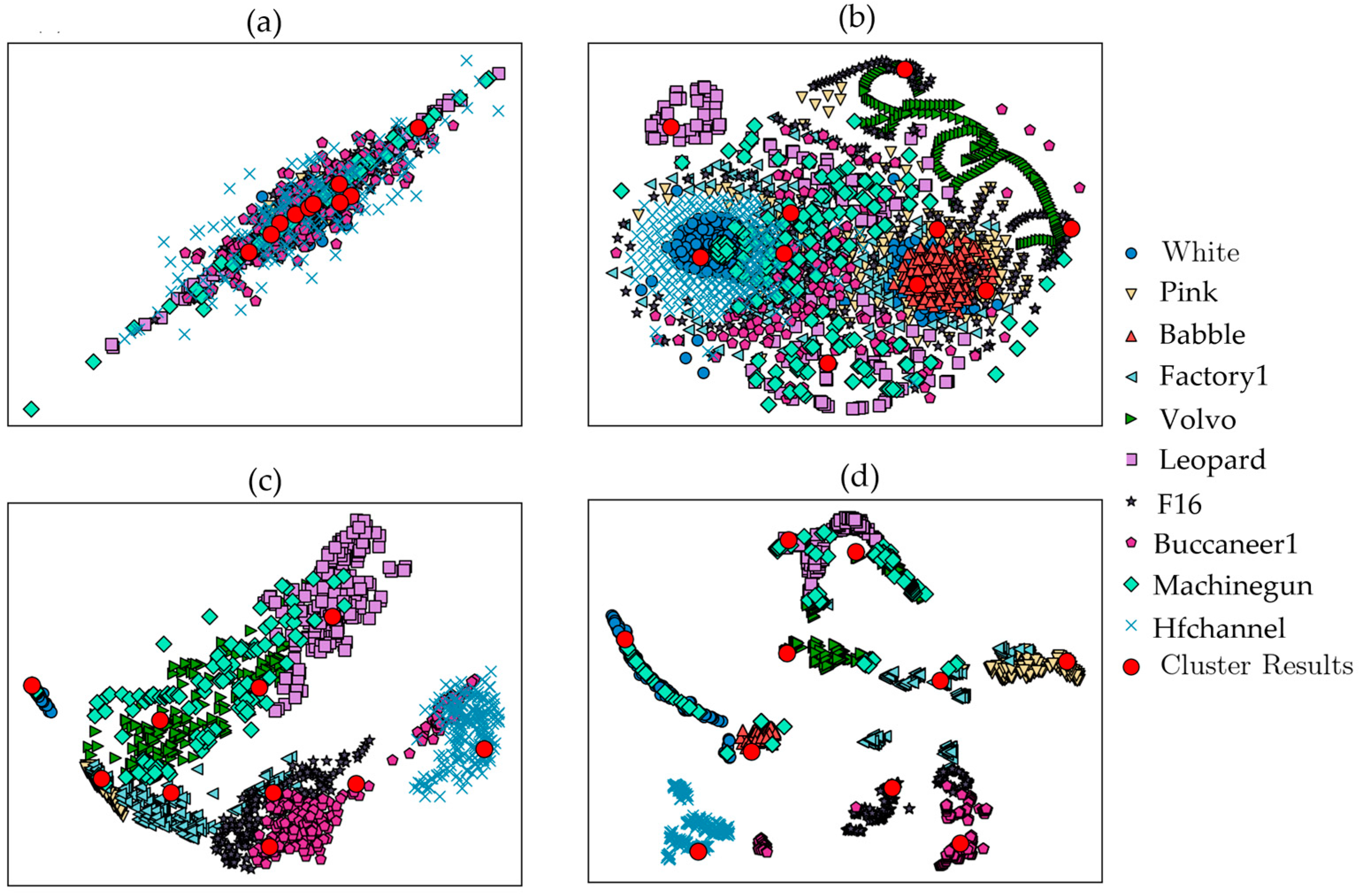
4.1. Clustering Result of Noise Data Set

The k-means++ cluster method was adopted to classify a noise dataset into different noise types. As the clustering algorithm is unsupervised learning, there is too much uncertainty for it to attain class labels. To evaluate the performance of the clustering algorithm used in this paper, class labels were assigned for different noise types. In this way, the effect of the clustering algorithm could be evaluated based on the following five indicators:

• V-measure indicates the harmonic mean of completeness and homogeneity. It is used to express the linear dependency between the cluster number and the sample number;
• Rand Index (RI) is the indicator to evaluate the similarity of two clusters;
• Adjusted Rand Index (ARI) is the improved version of RI, which is used to eliminate the influences of random label on RI;
• Normalized Mutual Information (NMI) is the normalized evaluation indicator to quantify the similarity between two clusters;
• Adjust Mutual Information (AMI) reflects the correlation between the cluster label and the ground truth label. It can be used for the consistency test of the clustering algorithm.

The values of five clustering evaluation indicators fall within the range of 0 to 1. Better performing clustering algorithms have larger indicator values.

This paper mainly studies the influence of noise data sampling length and decomposed IMF numbers on clustering performance. As shown by Figure 8a, the optimal noise sampling length is 512 from the perspective of noise clustering performance and computation. Before using the clustering algorithm to classify different types of noise, the raw noise data set was processed with VMD. A key factor affecting VMD feature extraction is the numbers of decomposed IMF. The clustering evaluation indicator values and computation times for different numbers of decomposed IMF are shown as Figure 8b. As shown in this figure, the optimal number of IMF was 6.

Figure 9 shows the superiority of the noise clustering algorithm based on the combination of VMD algorithm, PCA and K-means++; four groups of clustering results were determined as follows:

• (a) K-means++ for raw noise data: the k-means++ algorithm was directly performed on the raw noise dataset;
• (b) K-means++ for raw noise data with PCA: clustering analysis was performed with K-means++ algorithm for the noise data after PCA dimension reduction;
• (c) K-means++ for raw noise data with VMD: clustering analysis was performed with K-means++ algorithm for noise data after VMD feature extraction;
• (d) K-means++ for raw noise data with VMD/PCA: features of original noise data were extracted with VMD and PCA first and the clustering analysis was performed with K-means++.

As shown in Figure 9a, the result of noise classification clustering with raw data directly was not ideal. In comparison, as shown by Figure 9b, the clustering result was clearly improved when the noise data were initially processed with PCA dimension reduction. As shown by Figure 9c, the clustering result could also be improved significantly if noise classification clustering is performed after VMD noise feature extraction. Finally, the clustering algorithm based on the combination of VMD and PCA dimension reduction method delivers good performance in noise classification.

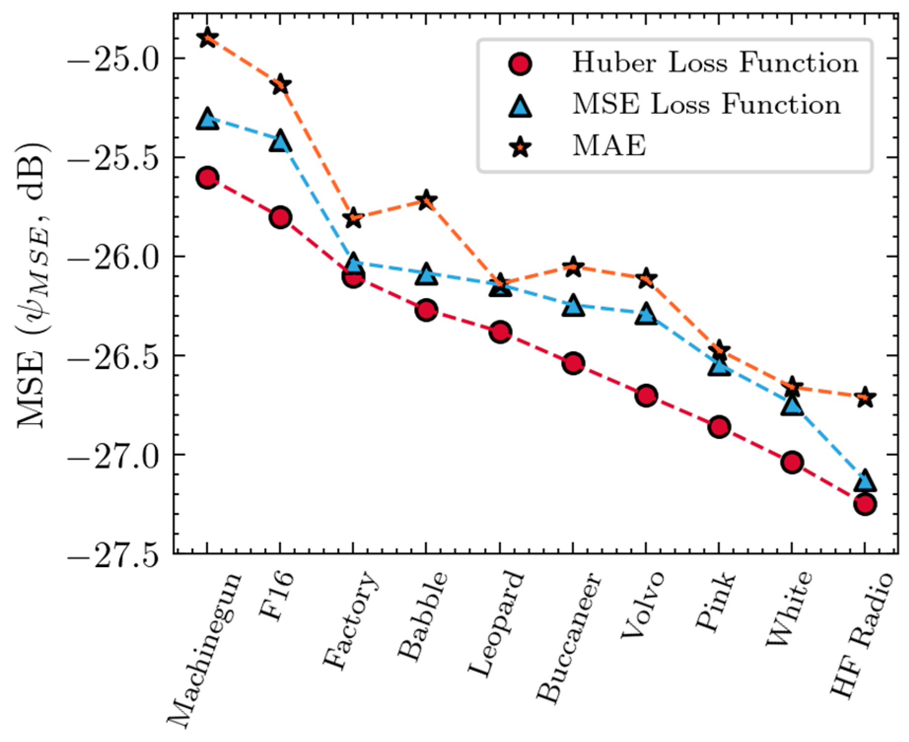
4.2. Architecture Determination and Regression Performance of GBDT

To compare the influences of different structural parameters on GBDT performance, the mean-square error (MSE), defined as ${\psi }_{MSE}=10{\log }_{10}\left\{e^2\left(n\right)\right\}$, was used. The performance of the GBDT (Gradient Boosting Decision Tree) regressor was mainly affected by the loss function, maximum depth and number of estimators of the individual regression estimators.The regression loss functions commonly used by GBDT include Mean Squared Error (MSE), Mean Absolute Error (MAE) and Huber error. The mean de-noise effects for three different loss functions in the 10 types of noise datasets are shown in Figure 10.

It can be seen from Figure 10 that the GBDT regressor with Huber loss function yields the smallest MSE ${\psi }_{MSE}$ for each of the 10 types of noise datasets. The MSE loss function curve is smooth and continuous and is, therefore, conducive to the iterative optimization through gradient descent method. However, it is sensitive to discrete points. In comparison, the MAE loss function is tolerant to discrete points, but it has high complexity in solving the gradient. As the fusion of MSE and MAE functions, Huber error can not only reduce the sensitivity to discrete points, but also allows differentiability in all situations. Therefore, the Huber error loss function is selected as the loss function of GBDT.

Influences of maximum depth and number of estimators on the regression performance of GBDT were examined. In order to simplify the determination architecture of GBDT, it was assumed that different noise types have the same GBDT structure. Using a trial-and-error method, the regression performance indicator MSE ${\psi }_{MSE}$ corresponding the maximum depth ranging from one to six and the number of estimators ranging from 100 to 700 were studied. Using factory noise as an example, the influence of maximum depth and number of estimators on the GBDT regression performance is shown in Figure 11. Therefore, the optimal maximum depth and number of estimators of GBDT used in this paper were four and 500, respectively.

4.3. Comparison between Proposed Method with Several Other Methods

The proposed method is compared against several other algorithms: least mean square (LMS) [28], recursive least square (RLS) [29], random forest (RF), support vector machine (SVM) and artificial neural network (ANN), in terms of the ANC performance. Generally, the LMS algorithm is simple and easy to implement with low complexity. But it has the disadvantages of a slow convergence rate and poor tracing performance. Recursive least square (RLS) algorithm has better convergence speed and tracing performance with higher computation complexity compared with LMS algorithm. Figure 12 shows the de-noising learning curves of proposed method, LMS, RLS, RF, SVM and ANN for 10 types of noise datasets with 500 steps iteration.

It can be seen from Figure 12 that the learning curve of the method proposed in this paper begins to converge at iteration step 75 which is much smaller than that of LMS algorithm. For the RLS algorithm, the convergence iteration step is 48. Although the convergence speed of the proposed method is not as fast as that of RLS, its maximum value of the learning curve is 8.08 dB, which is much less than that of RLS, 29.66 dB. This demonstrates that the proposed method has better stability compared with LMS and RLS. In addition, the convergence iteration steps for the learning curve of RF, SVM and ANN methods are 145, 58 and 80 respectively, which are not very different than that of the proposed method. However, the maximum value of the learning curve of RF, SVM and ANN methods is 26.23 dB, 29.51 dB and 28.25 dB respectively, which is much larger than the value of the proposed method. In addition, the steady-state attenuation result of the proposed method is −25.6 dB~−27.25 dB, and results of the LMS, RLS, RF, SVM and ANN methods are −17.8 dB~−24.08 dB, −17.5 dB~−24.52 dB, −22.47 dB~−26.57 dB, −22.05 dB~−25.83 dB and −23.37 dB~−26.61 dB, respectively. This shows that the proposed method has better noise attenuation using the 10 types of noise datasets. The reason for this is that the proposed method constructs a corresponding regressor according to the clustering results of different noise types, which greatly improves the noise attenuation effect.

4.4. Simulation Validation of Proposed Method

In order to further verify the effectiveness of the proposed method for ANC, the noise attenuation effect of machine gun noise is analyzed with the proposed method by formulating four simulation schemes shown in Figure 6 and using the sound pressure level (SPL) as the evaluation index. The noise attenuation effects of ANC in an obstacle-free rectangular enclosed space are shown in Figure 13a,b. It reveals that the SPL in the enclosed space is between 29.75 and 56.31 dB without ANC as shown in Figure 13a. However, with ANC based on proposed method, the SPL in the space is approximately −23.27 dB, as shown in Figure 13b.

For the simulation condition of rectangular enclosed space with obstacle, the SPL without ANC in the enclosed space is between 2.76 and 39.3 dB, as shown in Figure 13c. With ANC based on proposed method, the SPL at the noise control point is basically around −21.6 dB as shown Figure 13d. It demonstrates that the method proposed in this paper can well achieve the noise attenuation for rectangular enclosed space.

The simulation results of trapezoidal enclosed space are shown in Figure 14. The noise attenuation effects of ANC in an obstacle-free trapezoidal enclosed space are shown in Figure 14a,b. It reveals that the SPL in the enclosed space is basically between −7.49 and 27.28 dB without ANC as shown in Figure 14a. However, after the ANC using the proposed method, the SPL in the space is approximately −19.08 dB, as shown in Figure 14b.

For the simulation condition of trapezoidal enclosed space with obstacle, the SPL in the enclosed space is between −4.71 and 27.6 dB without ANC as shown in Figure 14c. With ANC based on proposed method, the SPL at the noise control point is approximately −15.48 dB, as shown Figure 14d. It also demonstrates that the method proposed in this paper can achieve the noise attenuation for trapezoidal enclosed space.

In another example, LMS, RLS, RF, SVM and ANN algorithms were used for ANC of machine gun noise using the four simulation schemes as above. Their noise attenuation effects are shown in Figure 15. The noise attenuation effect of the LMS algorithm for four simulation schemes are −13.47 dB, −10.9 dB, −7.78 dB and −2.75 dB respectively. The noise attenuation effect of the RLS algorithm for the four simulation schemes are −14.93 dB, −12.72 dB, −9.46 dB and −4.53 dB respectively. The noise attenuation effect of the RF algorithm for four simulation schemes are −16.96 dB, −14.5 dB, −11.06 dB and −6.59 dB respectively. The noise attenuation effect of the SVM algorithm for four simulation schemes are −17.86 dB, −14.77 dB, −11.72 dB and −7.54 dB respectively. The noise attenuation effect of ANN algorithm for four simulation schemes are −19.03 dB, −16.54 dB, −13.18 dB and −8.26 dB respectively. Therefore, it can be found that the noise attenuation effect of the proposed method is much better than that of algorithms of LMS, RLS, RF, SVM and ANN.

From the simulation results of the above four cases, it can be seen that with increasing spatial irregularity, it would be more difficult to achieve ANC, but the algorithm proposed in this paper can meet the actual needs of practical engineering applications on the whole. In future research, we will focus on algorithm research of ANC for a more irregular space and a more complex environment.

5. Conclusions

This paper proposes a novel method based VMD and GBDT for ANC. The proposed method decomposes different types of noise data by VMD and obtains the approximate entropy of each IMF. The clustering analysis is carried out on the output of VMD, based on the PCA dimension reduction method and k-means++ method. Then, different GBDT regression learners are built for different noise types and their structural parameters are optimized to achieve high-performance active noise control for different noise types. As shown by the simulation analysis, the result shows the VMD method could extract the inherent characteristics of different noises and greatly improve the clustering effect of different noise types. Meanwhile, the PCA is also used to extract the features of each IMF of noise, thereby further enhancing the clustering effect of k-means++. In addition, since the GBDT regression learner is built for every IMF of noise separately, high-performance ANC for different types of noise is acheived. Compared with ANC methods using a LMS algorithm and RLS algorithm, the proposed method has a better noise reduction effect. Four simulation schemes were conducted to verify the effectiveness of the proposed method for ANC. The simulation results revealed that the algorithm proposed in this paper can meet the actual needs of practical engineering applications on the whole. Therefore, the proposed method provides sound technical support for ANC of multiple noise sources.

References

1. Dragomiretskiy, K.; Zosso, D. Variational mode decomposition. IEEE Trans. Signal Process. 2014, 22, 531–534. [Google Scholar] [CrossRef]
2. Li, G.H.; Liu, F.; Yang, H. Research on feature extraction method of ship radiated noise with K-nearest neighbor mutual information variational mode decomposition, neural network estimation time entropy and self-organizing map neural network. Measurement 2022, 199, 111446. [Google Scholar] [CrossRef]
3. Yang, H.; Shi, W.S.; Li, G.H. Underwater acoustic signal denoising model based on secondary variational mode decomposition. Def. Technol. 2022, 3. [Google Scholar] [CrossRef]
4. Zhang, L.; Tang, J.T.; Li, G.; Chen, W.J. Audio magnetotelluric denoising via variational mode decomposition and adaptive dictionary learning. J. Appl. Geophys. 2022, 204, 104748. [Google Scholar] [CrossRef]
5. Wu, G.N.; Liu, G.C.; Wang, J.X.; Fan, P.P. Seismic random noise denoising using mini-batch multivariate variational mode decomposition. Comput. Intell. Neurosci. 2022, 2022, 2132732. [Google Scholar] [CrossRef] [PubMed]
6. Wu, H.; Zhang, B.; Lin, T.F.; Li, F.Y.; Liu, N.H. White noise attenuation of seismic trace by integrating variational mode decomposition with convolutional neural network. Geophysics 2019, 84, 307–317. [Google Scholar] [CrossRef]
7. Wei, H.R.; Qi, T.Y.; Feng, G.R.; Jiang, H.N. Comparative research on noise reduction of transient electromagnetic signals based on empirical mode decomposition and variational mode decomposition. Radio Sci. 2021, 56, 1–19. [Google Scholar] [CrossRef]
8. Mohanmmed, A.; Kora, R. A comprehensive review on ensemble deep learning: Opportunities and challenges. J. King Saud Univ. Comput. Inf. Sci. 2023, 35, 757–774. [Google Scholar] [CrossRef]
9. Kumarasamy, K.; Wenisch, S.M.; Balaji, S.; Suriya, L.J.J.; Jerlin, A.; Rajkumar, S.R. Improving impulse noise classification using ensemble learning methods. Adv. Intell. Syst. Comput. 2021, 1299, 187–199. [Google Scholar] [CrossRef]
10. Campagner, A.; Ciucci, D.; Cabitza, F. Aggregation models in ensemble learning: A large-scale comparison. Inf. Fusion 2023, 90, 241–252. [Google Scholar] [CrossRef]
11. Nguyen, T.N.A.; Nhu, Q.P.; Solanki, V.K. Novel noise filter techniques and dynamic ensemble selection for classification. Recent Adv. Comput. Sci. Commun. 2022, 15, 48–59. [Google Scholar] [CrossRef]
12. Ngo, G.; Beard, R.; Chandra, R. Evolutionary bagging for ensemble learning. Neurocomputing 2022, 510, e2020RS007135. [Google Scholar] [CrossRef]
13. Fauvel, K.; Fromont, É.; Masson, V.; Faverdin, P.; Termier, A. XEM: An explainable-by-design ensemble method for multivariate time series classification. Data Min. Knowl. Discov. 2022, 36, 917–957. [Google Scholar] [CrossRef]
14. González, S.; García, S.; Del Ser, J.; Rokach, L.; Herrera, F. A practical tutorial on bagging and boosting based ensembles for machine learning: Algorithms, software tools, performance study, practical perspectives and opportunities. Inf. Fusion 2020, 64, 205–237. [Google Scholar] [CrossRef]
15. Konstantinov, A.V.; Utkin, L.V. Interpretable machine learning with an ensemble of gradient boosting machines. Knowl.-Based Syst. 2021, 222, 106993. [Google Scholar] [CrossRef]
16. Friedman, J.H. Greedy function approximation: A gradient boosting machine. Ann. Stat. 2001, 29, 1189–1232. [Google Scholar] [CrossRef]
17. Nhat-Duc, H.; Van-Duc, T. Comparison of histogram-based gradient boosting classification machine, random Forest, and deep convolutional neural network for pavement raveling severity classification. Autom. Constr. 2023, 148, 104767. [Google Scholar] [CrossRef]
18. Ke, G.; Meng, Q.; Finley, T.; Wang, T.; Chen, W.; Ma, W.; Ye, Q.; Liu, T.-Y. LightGBM: A highly efficient gradient boosting decision tree. Adv. Neural Inf. Process. Syst. 2017, 30, 3149–3157. [Google Scholar]
19. Patri, A.; Patnaik, Y. Random forest and stochastic gradient tree boosting based approach for the prediction of airfoil self-noise. Proc. Comput. Sci. 2014, 46, 109–121. [Google Scholar] [CrossRef]
20. Li, L.; Dai, S.; Cao, Z.; Hong, J.; Jiang, S.; Yang, K. Using improved gradient-boosted decision tree algorithm based on Kalman filter (GBDT-KF) in time series prediction. J. Supercomput. 2020, 76, 6887–6900. [Google Scholar] [CrossRef]
21. Wu, S.L.; Wang, B.F.; Zhao, L.X.; Liu, H.S.; Geng, J.H. High-efficiency and high-precision seismic trace interpolation for irregularly spatial sampled data by combining an extreme gradient boosting decision tree and principal component analysis. Geophys. Prospect. 2022, 20224713147273. [Google Scholar] [CrossRef]
22. Yentes, J.M.; Hunt, N.; Schmid, K.K.; Kaipust, J.P.; McGrath, D.; Stergiou, N. The appropriate use of approximate entropy and sample entropy with short data sets. Ann. Biomed. Eng. 2013, 41, 349–365. [Google Scholar] [CrossRef] [PubMed]
23. Trendafilov, N.; Gallo, M. PCA and other dimensionality-reduction techniques. In International Encyclopedia of Education, 4th ed.; Elsevier: Amsterdam, The Netherlands, 2023; pp. 509–599. [Google Scholar] [CrossRef]
24. Vinh, N.X.; Epps, J.L.; Bailey, J. Information theoretic measures for clusterings comparison: Variants, properties, normalization and correction for chance. J. Mach. Learn. Res. 2010, 11, 2837–2854. [Google Scholar]
25. Varga, A.; Steeneken, H.J.M. Assessment for automatic speech recognition: II. NOISEX-92: A database and an experiment to study the effect of additive noise on speech recognition systems. Speech Commun. 1993, 3, 247–251. [Google Scholar] [CrossRef]
26. Zhang, Y.D.; Yang, Z.J.; Lu, H.M.; Zhou, X.X.; Phillips, P.; Liu, Q.M.; Wang, S.H. Facial emotion recognition based on biorthogonal wavelet entropy, fuzzy support vector machine, and stratified cross validation. IEEE Access 2016, 4, 8375–8385. [Google Scholar] [CrossRef]
27. Scheibler, R.; Bezzam, E.; Dokmanic, I. Pyroomacoustics: A Python package for audio room simulations and array processing algorithms. In Proceedings of the 2018 IEEE International Conference on Acoustics, Speech and Signal Processing (ICASSP), Calgary, AB, Canada, 15–20 April 2018. [Google Scholar] [CrossRef]
28. Chu, Y.J.; Zhao, S.P.; He, L.B.; Niu, F. Wind noise suppression in filtered-x least mean squares-based active noise control systems. J. Acoust. Soc. Am. 2022, 152, 3340–3345. [Google Scholar] [CrossRef]
29. Wu, L.F.; Qiu, X.J.; Burnett, L.S.; Guo, Y.C. A recursive least square algorithm for active control of mixed noise. J. Sound Vib. 2015, 339, 1–10. [Google Scholar] [CrossRef]
Figure 1. Block diagram of active noise control based on VMD and GBDT.
Applsci 13 05436 g001
Figure 2. Feature extraction based on VMD, PCA and k-means++.
Applsci 13 05436 g002
Figure 3. The construction of GBDT for ANC.
Applsci 13 05436 g003
Figure 4. The partition method for different types of noise data.
Applsci 13 05436 g004
Figure 5. ANC simulation schematic diagram.
Applsci 13 05436 g005
Figure 6. Four simulation schemes for the ANC, (a) Obstacle-free Rectangular Enclosed Space (b) Rectangular Enclosed Space with Obstacle (c) Obstacle-free Trapezoidal Enclosed Space (d) Trapezoidal Enclosed Space with Obstacle.
Applsci 13 05436 g006
Figure 7. Impulse response of the primary path for different noise type under four simulation schemes.
Applsci 13 05436 g007
Figure 8. The influence of noise data sampling length and number of IMF on clustering performance.
Applsci 13 05436 g008
Figure 9. Clustering results of different types of noise datasets with different methods, (a) K-means++ for Raw Noise Data, (b) K-means++ for raw noise data with PCA, (c) K-means++ for raw noise data with VMD, (d) K-means++ for raw noise data with VMD/PCA.
Applsci 13 05436 g009
Figure 10. The de-noise effects of GBDT with MSE, MAE and Huber loss functions.
Applsci 13 05436 g010
Figure 11. The influence of maximum depth and number of estimators on the GBDT regression performance.
Applsci 13 05436 g011
Figure 12. The learning curves of proposed method and several other methods.
Applsci 13 05436 g012
Figure 13. The ANC simulation results of rectangular enclosed space, (a) SPL without ANC for Obstacle-free Rectangular Enclosed Space, (b) SPL with ANC for Obstacle-free Rectangular Enclosed Space, (c) SPL without ANC for Rectangular Enclosed Space with Obstacle, (d) SPL with ANC for Rectangular Enclosed Space with Obstacle.
Applsci 13 05436 g013
Figure 14. The ANC simulation results of trapezoidal enclosed space, (a) SPL without ANC for Obstacle-free Trapezoidal Enclosed Space, (b) SPL with ANC for Obstacle-free Trapezoidal Enclosed Space, (c) SPL without ANC for Trapezoidal Enclosed Space with Obstacle (d) SPL with ANC for Trapezoidal Enclosed Space with Obstacle.
Applsci 13 05436 g014
Figure 15. The ANC simulation results of proposed methods and several other methods.
Applsci 13 05436 g015