Wind Speed Measurement via Visual Recognition of Wind-Induced Waving Light Stick Target

Abstract

Wind measurement in confined spaces is a challenge due to the influence of the dimensions of anemometers in intrusive flow-field measurements where the anemometer probes directly contact and influence the near-probe flow field. In this work, a new wind speed detection methodology is proposed based on wind-induced motion of a stick via vision-based recognition. The target’s displacement in pixel coordinates is mapped to its angular displacement in world coordinates to derive wind speed and direction information by applying the calibration coefficients. Simulation experiments were carried out to validate the model, the error of which was within an angular displacement of 4.0° and 3.0° for wind speed and direction detections, respectively. When applied to the measurement of wind speed in the inner equipment cabin of a stationary high-speed train, the error was within ±1.1 m/s in terms of average RMSE. Thus, the proposed method provides an accurate and economic option for monitoring 2D wind in a confined space.

1. Introduction

Computer vision is a multidisciplinary field of study that involves enabling computers to gain understanding of data (usually digital images and videos) and, in the process, acquire, process, and extract useful information for decision making [1]. Some of the popular areas of application of computer vision techniques include robotics [2], autonomous vehicles [3], and environmental monitoring [4]. The measurement of wind speed and direction is a crucial aspect of environmental monitoring, especially for areas such as fault diagnosis [5] and wind energy monitoring [6]. Meteorologists also use wind information for climate pattern and climate trend research [6]. While the accuracy of the technique employed in measuring this highly dynamic parameter (wind speed) is central to the integrity of the measurement, factors such as cost and area of application can lead to differences in choosing an appropriate technique, since different techniques may have application-specific strengths and weaknesses [7]. One application where cup anemometers may be more suitable than pitot tube anemometers is in measuring wind speeds near the ground or in complex terrain [8]. This is because cup anemometers are less affected by turbulence and changes in wind direction than pitot tube anemometers, which can be affected by eddies and vortices in the flow [9,10]. On the other hand, pitot tube anemometers may be more suitable for measuring airspeed in aircraft, unmanned aerial vehicles (UAVs), or other fluid flows where the total velocity, including horizontal and vertical components, is of interest [11]. Therefore, computer vision hardware and algorithms similarly offer a strong alternative to other wind measurement systems, alongside the expected comparative application-specific merits. They are usually applied in areas where highly accurate, cost-effective, real-time, and non-intrusive approaches are desired [12,13].

Following fundamental contributions such as the simple mechanical wind indicator developed by Robert Hooke (1635–1703) and Sir Christopher Wren (1632–1723), which measured wind speed based on the directional deflection of a hanging plate oriented into the direction from which the wind was blowing [14], more complex mechanical and ultrasonic wind sensors were developed. The cup anemometer for instance, has become a widely used device for accurate horizontal wind speed measurement, improving upon the previous techniques [15]. The use of pitot tubes in airspeed measurement has also gained prominence because of their advantages in measuring fluid flow where the use of anemometers is impractical, in addition to their characteristic low cost, minimal friction losses, simple set up, and ease of installation merits [16,17]. In the aviation industry and wind tunnel ducts, pitot tubes can measure static and dynamic pressure of the prevailing wind, which is then converted to airspeed using the Bernoulli equation. Despite their many advantages however, they are sensitive to wind flow direction, can become clogged by particles when operating in dirty environments, and do not work well in low or medium wind speed environments [18].

In recent years, computer vision techniques have increasingly been used for wind measurement due to their accuracy, efficiency, and cost effectiveness. Existing studies have considered employing machine learning techniques such as convolutional neural networks (CNNs) and recurrent neural networks (RNNs) for wind measurement [19,20,21,22]. Notably, Yang et al. [21] proposed a novel wind measurement system for an unmanned sailboat based on computer vision (CV). The system consists of an airflow rope, a camera, and a computing platform. It measures the wind speed and direction by analyzing the fluttering of the airflow rope using a combination of a CNN and an RNN. Other methods which do not rely on artificial intelligence have also been reported [19,20,21]. Among these, the work by Gunnlaugsson et al. [22] is notable. The paper describes the design and construction of a telltale wind indicator for the Mars Phoenix lander, which was sent to Mars by NASA to study the Martian arctic environment. The wind measurement system involves a video camera focused on the movement of a suspended lightweight Kapton tube, based on which wind measurement, direction, and turbulence can be estimated.

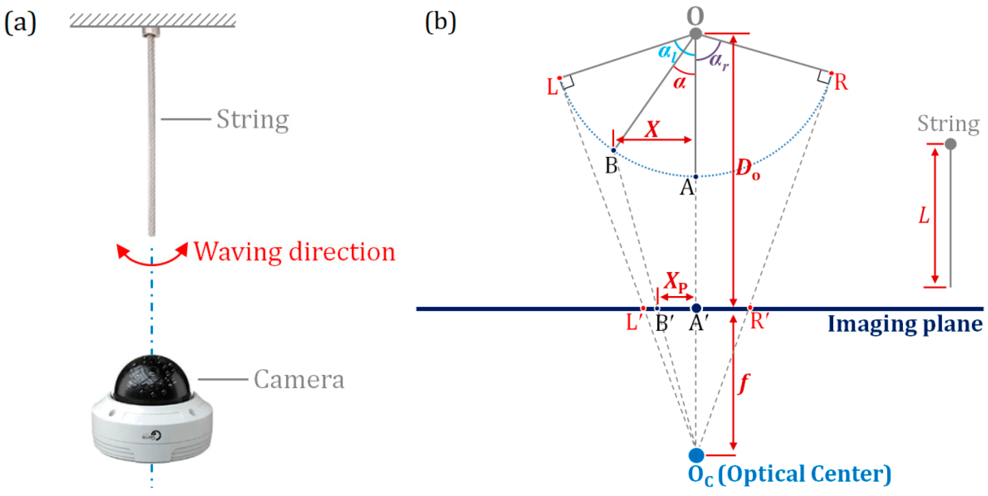
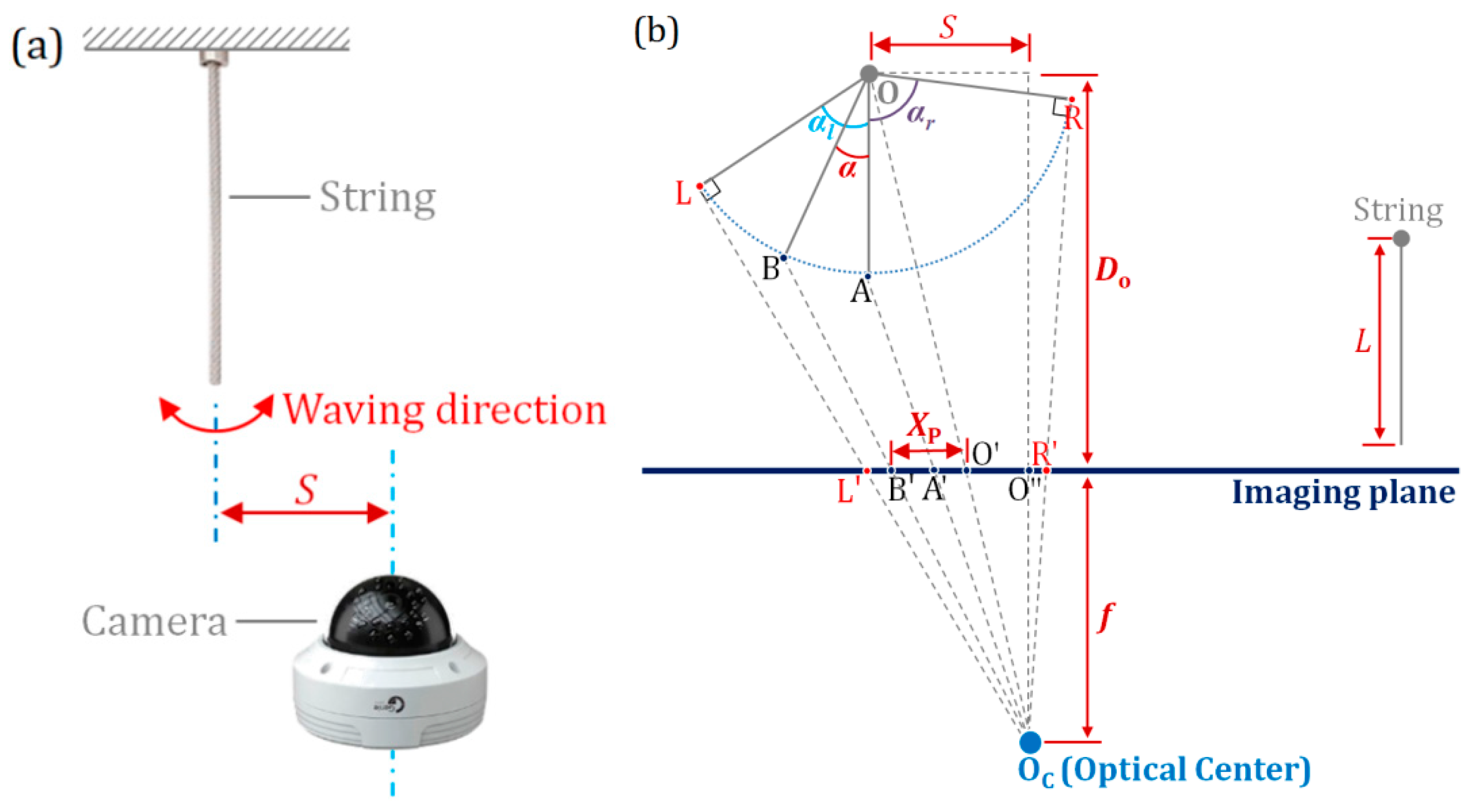
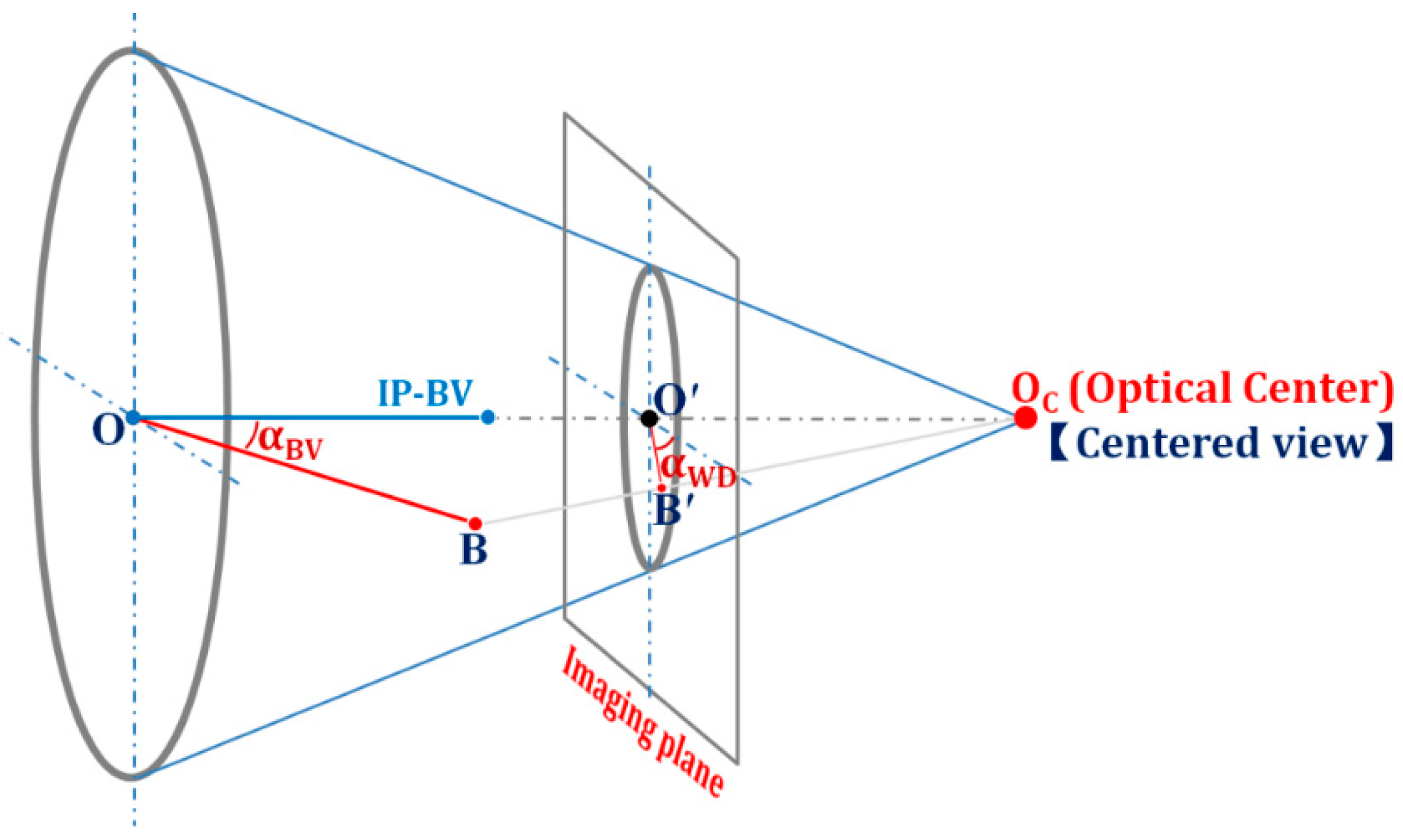
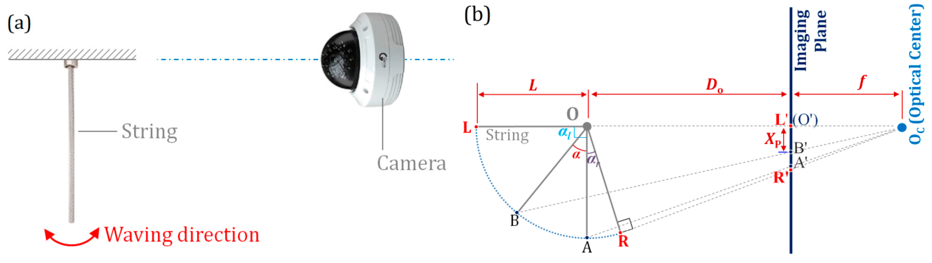
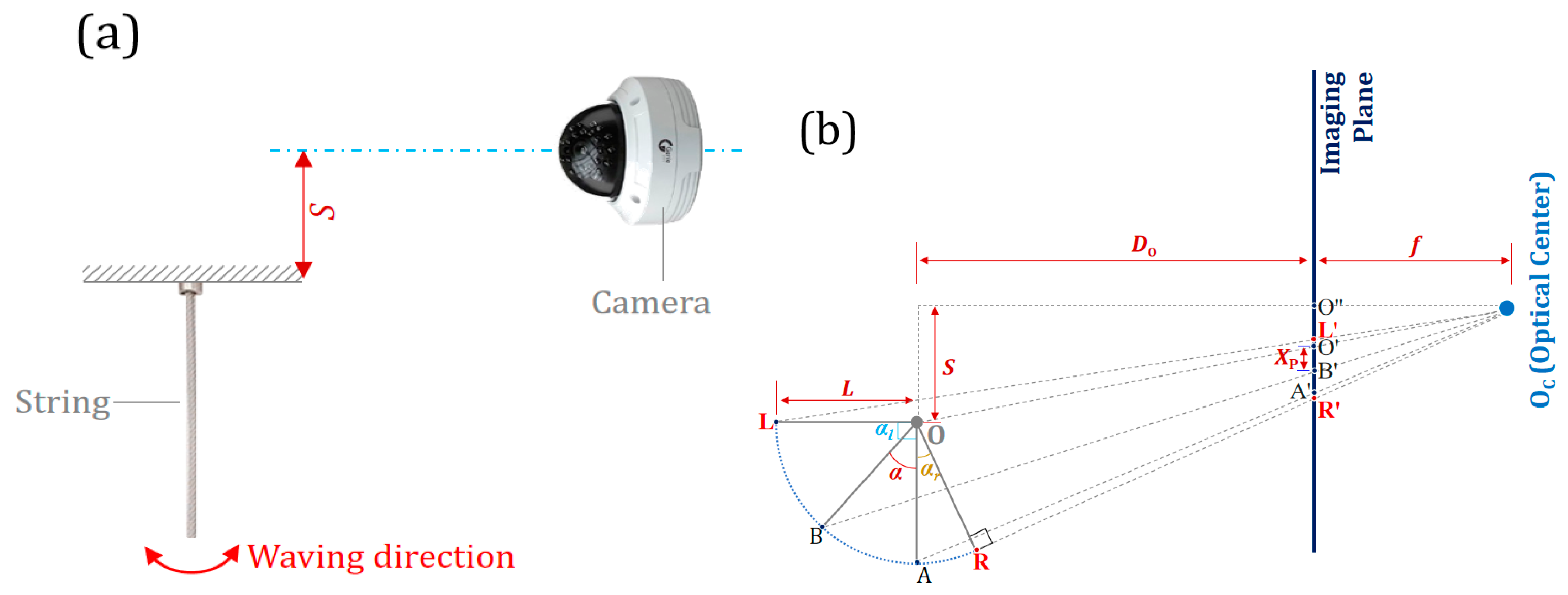
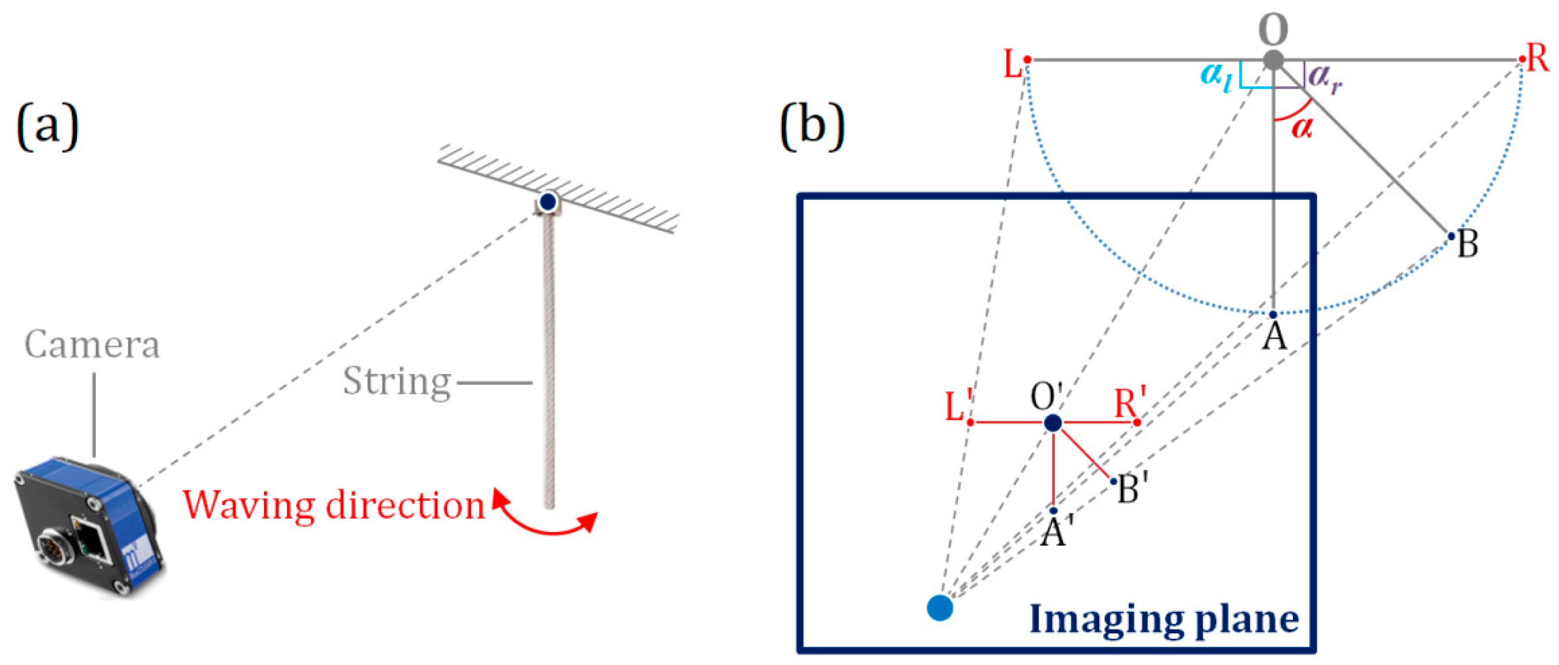
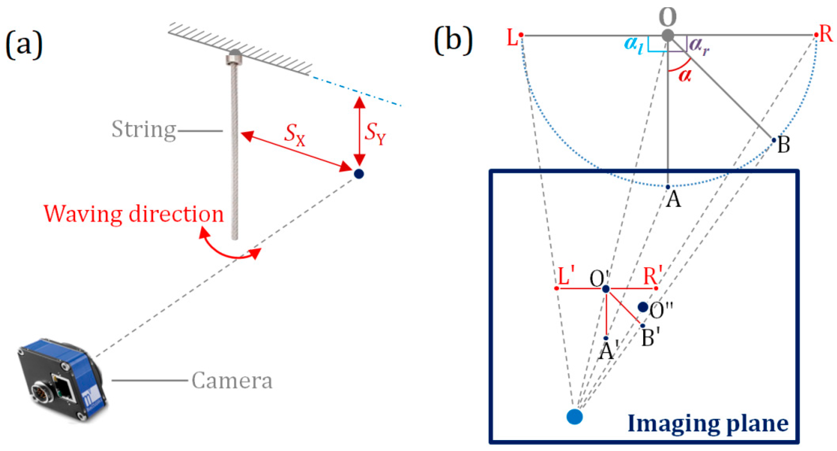
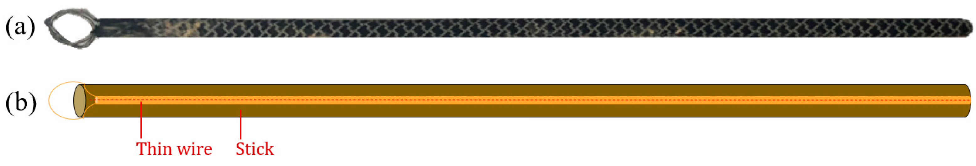
This paper proposes a computer-vision-based wind speed and direction measurement methodology for horizontal wind speed measurement in small, enclosed areas such as a stationary train equipment cabin. The proposed system consists of a single camera focused on a lightweight stick target that swings according to wind strength and direction. The pinhole camera model is implemented to model the relationship between the real-world angular displacement of the target and its corresponding displacement in the image plane when the camera is positioned relative to the lightweight stick target in front, side, and bottom orientations. The method combines the advantages of being lightweight, and having less intrusion on the flow field, small size, low cost, simple set up, and acceptable accuracy. These qualities make the proposed method particularly promising for two-directional wind speed measurement in enclosed areas.

The comparative advantages of the proposed method compared to traditional methods such as the plate anemometer immediately stand out. Compared to the plate anemometer, for instance, the proposed method is less intrusive, less prone to human error, and occurs in real time. Furthermore, the proposed method is not as sensitive to flow direction as the pitot tube and cup anemometer which are, in addition, more flow-intrusive. At the core of our proposed measurement methodology is the real-time detection of the lightweight stick, based on which wind speed and direction can be estimated. Therefore, our proposed method and the works of Yang et al. [21] and Gunnlaugsson et al. [22] also share similarities in that all involve vision-based detection of the fluttering, waving, or movement of some target. However, the former’s method is based on laboratory training data with an ultrasonic sensor as the reference device. This creates significant room for bias against the real working environment of the boat (sea and/or ocean). Although the authors attempted to address the problem, it remained an important limitation, as they admitted. The proposed method addresses this by establishing a well-defined relationship between the real-world movement of the target and its corresponding displacement in camera coordinates to allow for real-time measurement that directly depends on the active scene condition. Furthermore, in the application of the proposed method, several targets were lined across the breadth of the enclosed space in different positions, and focused on the same camera, to attain high accuracy and robustness, as suggested by Yang et al. [21]. The latter’s method relies on the kinetic energy of the target and several empirical factors. Moreover, the determination of wind speed wholly depends on the relative tilt of the target, which necessitates dependence on one orientation where the camera plane is parallel to the movement of the target. If the camera were to be placed at an angle to the telltale, the output tilt angle would be incorrect, leading to incorrect wind speed measurement. In contrast, the proposed method relies on the geometric attitude of the target and attempts to address the heavy dependence on the relative camera–target orientation by formulating four different camera orientation scenarios, including one that couples multiple orientations.

Thus, we propose a wind speed and direction measurement method based on the movement of a lightweight stick. Detailed formulations are given for different camera orientations to correctly capture the target’s movement. Based on this displacement and together with the wind tunnel calibration coefficients, the wind speed and direction are determined. The method is applied to wind speed measurement in a stationary train equipment cabin, and compared with standard pitot measurements, showing good agreement. The method combines the advantages of being lightweight, and having less intrusion with the near flow field, small size, low cost, simple set up, and acceptable accuracy. These qualities make the proposed method particularly promising for two-directional wind speed measurement in enclosed environments such as the inner equipment cabin of railway trains. 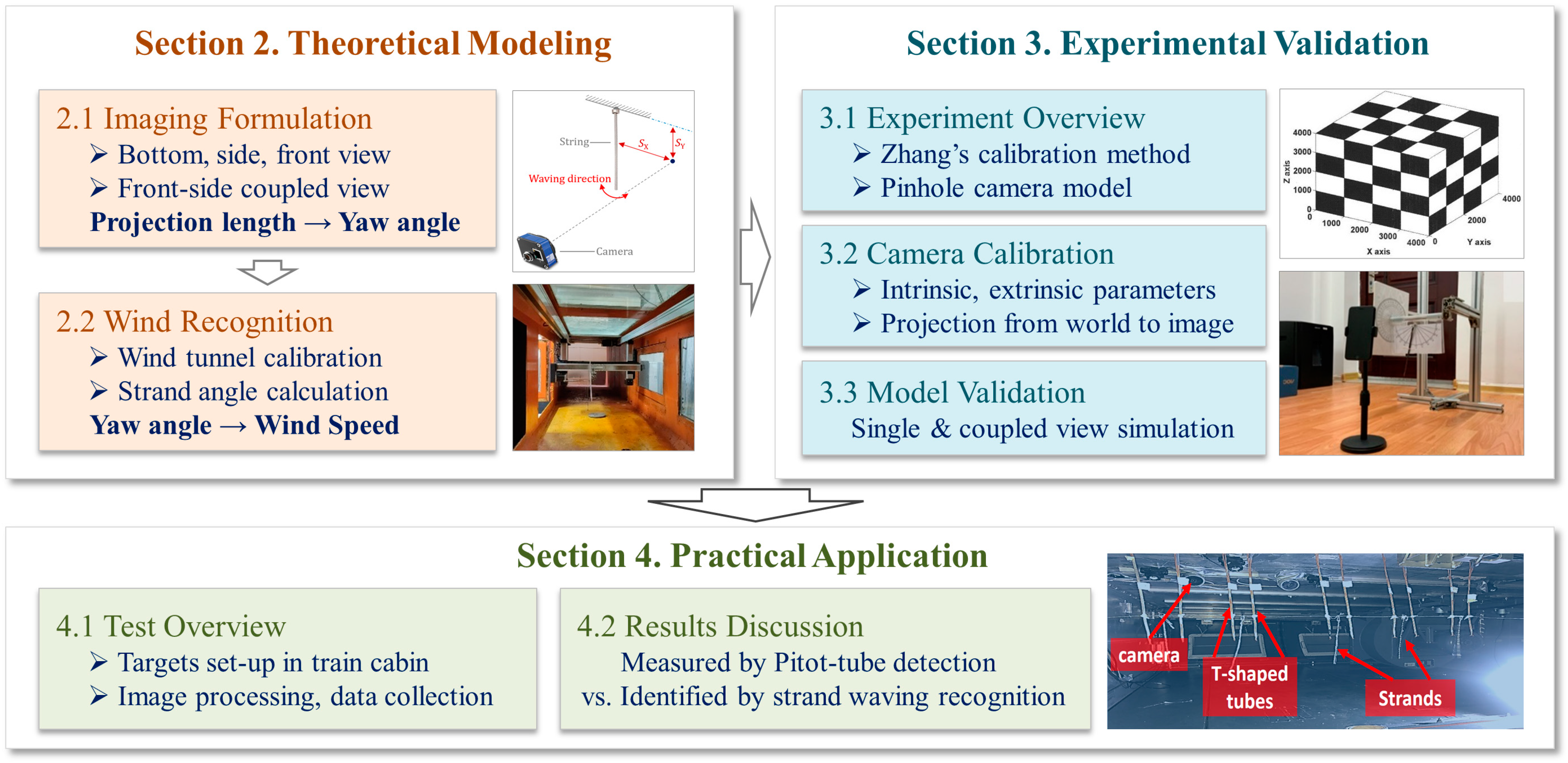Figure 1 presented below is the technical route of the paper.

2. Theoretical Modeling

2.1. Imaging Formulation

To measure horizontal wind speed, the proposed vision-based measurement system relies on (1) the corresponding (angular) displacement of the real-world light-stick target in the camera image plane and (2) the coefficient relating this displacement to wind speed magnitude. To achieve the first, the pinhole camera model is used to model the target such that the captured target’s displacement in the image plane can be mapped to the real-world angular displacement of the target. Then, the target is calibrated in a wind tunnel experiment to determine the coefficient relating its angular displacement to the wind speed magnitude. In this way, the prevailing horizontal wind speed can be determined by the product of the angular displacement of the target as obtained by the camera, and the wind speed–displacement coefficient as obtained from the calibration experiment.

2.1.1. Bottom View

The theoretical model at the bottom view is given in centered and deviated imaging, where in centered imaging, the initial stick line passes through the optical center, whereas in deviated imaging, there is a distance S between the stick line and optical center.

In centered imaging at the bottom view, the fixed end of the stick is denoted as O, and the moving end rotates in a circular trajectory. The stick yaw angle is defined with respect to its initial vertical position as α. The imaging length on the projection plane is denoted as X_P. Parameters including the stick length L, camera focal length f, and object distance D_O of the stick fixed end are all measured and calibrated before detection as in Figure 2.

When the stick is propelled by horizontal wind and rotates in different yaw angles from the beginning, the imaging length X_P on the imaging plane experiences a rise until the link between the optical center and stick moving end becomes normal to the stick itself. The corresponding yaw angle is described as α_l. After the perpendicular point L, the imaging length X_P drops as the yaw angle still climbs, even if the stick is lifted up to the horizontal limit. Accordingly, the symmetrical perpendicular point at the right side is denoted as R when the detected yaw angle reaches its limit of α_r in Figure 3b.

When the stick rotates in yaw angle α, the imaging length on imaging plane is defined as X_P =|A′B′|. The distance between moving end B and optical centerline, denoted as X, follows a linear relation with the imaging length X_P considering triangle similarity in Equation (1).

$$\frac{X_{\mathrm{P}}}{f}=\frac{X}{D_{\mathrm{O}}-L·\mathrm{c}\mathrm{o}\mathrm{s}\alpha +f}=\frac{L·\sin \alpha }{D_{\mathrm{O}}-L·\mathrm{c}\mathrm{o}\mathrm{s}\alpha +f}$$

(1)

The yaw angle α can then be expressed in Equation (2) as below.

$$\alpha ={\tan }^{-1}\left(\frac{\left(D_{\mathrm{O}}+f\right)·f·X_{\mathrm{P}}-X_{\mathrm{P}}·\sqrt{\left[L^2-{\left(D_{\mathrm{O}}+f\right)}^2\right]{·X_{\mathrm{P}}}^2+L^2·f^2}}{\left(D_{\mathrm{O}}+f\right)·{X_{\mathrm{P}}}^2+f·\sqrt{\left[L^2-{\left(D_{\mathrm{O}}+f\right)}^2\right]{·X_{\mathrm{P}}}^2+L^2·f^2}}\right)$$

(2)

The critical yaw angle is defined as α_l at left and α_r at right when the maximum imaging length occurs at the tangential location. In the right triangle OLO_C, the yaw angle range can be written as in Equation (3) below.

$${\alpha }_{\mathrm{l}}=-{\alpha }_{\mathrm{r}}={\cos }^{-1}\left(\frac{L}{D_O+f}\right)$$

(3)

where the positive angle is defined as clockwise, and negative is defined as anti-clockwise rotation.

Following the centered imaging case, similar formulations are hereby presented for the deviated imaging case where there is a deviation S between the camera optical center and the pure vertical state of the stick (Figure 3). According to triangle similarity, we have:

$$\begin{gathered} \frac{\left|{\mathrm{O}}^{″}{\mathrm{O}}^{\prime }\right|}{f}=\frac{S}{D_O+f} \\ \frac{\left|{\mathrm{O}}^{″}{\mathrm{B}}^{\prime }\right|}{f}=\frac{S+L·\sin \alpha }{D_O-L·\cos \alpha +f} \end{gathered}$$

(4)

The imaging length variation X_P can be formulated in Equations (3)–(6) as below.

$$\frac{X_{\mathrm{P}}}{f}=\frac{S+L·\sin \alpha }{D_O-L·\cos \alpha +f}-\frac{S}{D_O+f}$$

(5)

The tangent of the yaw angle in Equation (5) can thus be written as:

$$\alpha ={\tan }^{-1}\left(\frac{f·{\left(D_{\mathrm{O}}+f\right)}^3·X_{\mathrm{P}}-\left[\left(D_{\mathrm{O}}+f\right)·X_{\mathrm{P}}+S·f\right]·\sqrt{\mathrm{g}\left(X_{\mathrm{P}}\right)}}{{\left(D_{\mathrm{O}}+f\right)}^3·X_{\mathrm{P}}^2+S·f·{\left(D_{\mathrm{O}}+f\right)}^2·X_{\mathrm{P}}+f·\left(D_{\mathrm{O}}+f\right)·\sqrt{\mathrm{g}\left(X_{\mathrm{P}}\right)}}\right)$$

(6)

where:

$$g\left(X_{\mathrm{P}}\right)=\left[L^2{·\left(D_O+f\right)}^2-{\left(D_O+f\right)}^4\right]·X_P^2+2f·S·L^2·\left(D_O+f\right)·X_{\mathrm{P}}+\left[S^2+{\left(D_O+f\right)}^2\right]·f^2·L^2$$

(7)

From $\mathrm{\angle }\mathrm{L}\mathrm{O}{\mathrm{O}}_{\mathrm{C}}$ and ∠AOO_C:

$$\mathrm{\angle }\mathrm{L}\mathrm{O}{\mathrm{O}}_{\mathrm{C}}=\mathrm{\angle }\mathrm{R}\mathrm{O}{\mathrm{O}}_{\mathrm{C}}={\tan }^{-1}\left(\frac{\sqrt{{\left(D_O+f\right)}^2+S^2-L^2}}{L}\right)$$

(8)

$$\mathrm{\angle }\mathrm{A}\mathrm{O}{\mathrm{O}}_{\mathrm{C}}=\mathrm{\angle }\mathrm{O}{\mathrm{O}}_{\mathrm{C}}{\mathrm{O}}^{″}={\tan }^{-1}\left(\frac{S}{D_O+f}\right)$$

(9)

The yaw angle range limit α_r and α_l can thus be determined by:

$${\alpha }_{\mathrm{l}}=\mathrm{\angle }\mathrm{L}\mathrm{O}{\mathrm{O}}_{\mathrm{C}}-\mathrm{\angle }\mathrm{A}\mathrm{O}{\mathrm{O}}_{\mathrm{C}}={\tan }^{-1}\left(\frac{-L·S+\left(D_{\mathrm{O}}+f\right)·\sqrt{{\left(D_{\mathrm{O}}+f\right)}^2+S^2-L^2}}{L·\left(D_{\mathrm{O}}+f\right)+S·\sqrt{{\left(D_{\mathrm{O}}+f\right)}^2+S^2-L^2}}\right)$$

(10)

$${\alpha }_{\mathrm{r}}=\mathrm{\angle }\mathrm{R}\mathrm{O}{\mathrm{O}}_{\mathrm{C}}+\mathrm{\angle }\mathrm{A}\mathrm{O}{\mathrm{O}}_{\mathrm{C}}={\tan }^{-1}\left(\frac{L·S+\left(D_{\mathrm{O}}+f\right)·\sqrt{{\left(D_{\mathrm{O}}+f\right)}^2+S^2-L^2}}{L·\left(D_{\mathrm{O}}+f\right)-S·\sqrt{{\left(D_{\mathrm{O}}+f\right)}^2+S^2-L^2}}\right)$$

(11)

where α_l and α_r are as previously defined.

In bottom view where the initial stick position and the yaw angle are respectively denoted as ‘IP-BV’ and α_BV (Figure 4), the yaw angle α_IP-BV is calculated by substituting the imaging length |O′B′| into X_P, as in Equations (2) and (6), respectively, for centered and deviated bottom view. Formulations are given in Equation (12) as below:

$$\begin{gathered} X_{\mathrm{P}}=\left|{\mathrm{O}}^{\prime }{\mathrm{B}}^{\prime }\right|=\sqrt{{\left(X_{{\mathrm{O}}^{\prime }}-X_{{\mathrm{B}}^{\prime }}\right)}^2+{\left(Y_{{\mathrm{O}}^{\prime }}-Y_{{\mathrm{B}}^{\prime }}\right)}^2} \\ {\alpha }_{\mathrm{W}\mathrm{D}}={\mathrm{c}\mathrm{o}\mathrm{s}}^{-1}\left(\frac{X_{{\mathrm{B}}^{\prime }}}{\sqrt{{\left(X_{{\mathrm{O}}^{\prime }}-X_{{\mathrm{B}}^{\prime }}\right)}^2+{\left(Y_{{\mathrm{O}}^{\prime }}-Y_{{\mathrm{B}}^{\prime }}\right)}^2}}\right) \end{gathered}$$

(12)

2.1.2. Side View

Similar to the case of the bottom view, the theoretical model in side view is given in centered and deviated imaging. The projection length on the imaging plane is denoted as X_P, as in Figure 5. Other parameters are defined the same as in bottom view.

The physics of the motion of the stick are similar to the preceding bottom view case where it has been adequately described.

By triangle similarity, we have:

$$\frac{X_{\mathrm{P}}}{f}=\frac{X}{D_{\mathrm{O}}+L·\mathrm{s}\mathrm{i}\mathrm{n}\alpha +f}=\frac{L·\mathrm{c}\mathrm{o}\mathrm{s}\alpha }{D_{\mathrm{O}}+L·\mathrm{s}\mathrm{i}\mathrm{n}\alpha +f}$$

(13)

The yaw angle α can then be expressed as in Equation (14) below.

$$\alpha ={\tan }^{-1}\left(\frac{-{(D}_{\mathrm{O}}+f)·{X_{\mathrm{P}}}^2+f·\sqrt{\left[L^2-{\left(D_{\mathrm{O}}+f\right)}^2\right]{·X_{\mathrm{P}}}^2+L^2·f^2}}{f·(D_{\mathrm{O}}+f)·X_{\mathrm{P}}+X_{\mathrm{P}}·\sqrt{\left[L^2-{\left(D_{\mathrm{O}}+f\right)}^2\right]{·X_{\mathrm{P}}}^2+L^2·f^2}}\right)$$

(14)

The critical yaw angles α_r and α_l remain as previously defined, and are given in Equation (15) as:

$$\begin{gathered} {\alpha }_{\mathrm{l}}=\frac{\pi }{2} \\ {\alpha }_{\mathrm{r}}=\frac{\pi }{2}-{\tan }^{-1}\left(\frac{\sqrt{{\left(D_O+f\right)}^2-L^2}}{L}\right) \end{gathered}$$

(15)

In the case where there is a deviation S between the camera optical center and the pure vertical state of the stick (Figure 6), the imaging model is extended to accommodate the range of view.

Again, by triangle similarity, we have:

$$\begin{gathered} \frac{\left|{\mathrm{O}}^{″}{\mathrm{B}}^{\prime }\right|}{f}=\frac{(S+L\cos \alpha )}{D_O+f+L\sin \alpha } \\ \frac{\left|O^{″}{O}^{\prime }\right|}{f}=\frac{S}{D_O+f} \end{gathered}$$

(16)

The imaging length variation $X_{\mathrm{P}}$ can then be formulated in Equation (17) as below.

$$\frac{X_P}{f}=\frac{(S+L\cos \alpha )}{D_O+f+L\sin \alpha }-\frac{S}{D_O+f}$$

(17)

By trigonometric manipulations, the tangent of the yaw angle in Equation (18) is written as:

$$\alpha ={\tan }^{-1}\left(\frac{-{\left(D_O+f\right)}^3·{X_P}^2-S·f·{\left(D_O+f\right)}^2{·X}_P+(D_O+f)·f·\sqrt{g\left(X_P\right)}}{f·{\left(D_O+f\right)}^3·X_P+(\left(D_O+f\right)·X_P+S·f)·\sqrt{g\left(X_P\right)}}\right)$$

(18)

where the function g(X_P) under the square root is defined as:

$$g\left(X_{\mathrm{P}}\right)=\left[L^2{·\left(D_O+f\right)}^2-{\left(D_O+f\right)}^4\right]·X_P^2+2f·S·L^2·\left(D_O+f\right)·X_P+\left[S^2+{\left(D_O+f\right)}^2\right]·f^2·L^2$$

(19)

To solve for the α_r and α_l we consider $∆$OBO_C and $∆$OLO_C where:

$$\angle AOB={\tan }^{-1}\left(\frac{D_O+f}{S}\right)$$

(20)

$$\angle {\mathrm{B}\mathrm{O}\mathrm{O}}_C={\tan }^{-1}\left(\frac{\sqrt{{{\left(D_O+f\right)}^2+S}^2-L^2}}{L}\right)$$

(21)

The yaw angle range limit α_r and α_l can then be given according to Equations (22) and (23), respectively, below:

$${\alpha }_{\mathrm{l}}=\frac{\pi }{2}$$

(22)

$${\alpha }_{\mathrm{r}}=-{\tan }^{-1}\left(\frac{S·\sqrt{{{\left(D_O+f\right)}^2+S}^2-L^2}+L·\left(D_O+f\right)}{S·L-\left(D_O+f\right)·\sqrt{{{\left(D_O+f\right)}^2+S}^2-L^2}}\right)$$

(23)

2.1.3. Front View

The theoretical model in front view is also given in centered and deviated imaging, where in centered imaging, the line between restrained stick end and optical center is perpendicular to the imaging plane. In deviated imaging, there is a deviation between the restrained stick end and the optical centerline, as well as the geometrical center of the imaging plane.

In front view, the projection length is proportional to the stick length, as in Figure 7. Parameters are defined the same as in bottom view, all measured and calibrated before detection.

The yaw angle is calculated by the slopes of two lines at beginning and waved positions in Equation (24) as below.

$$\alpha ={\tan }^{-1}\left(\frac{k_{B^{\prime }}-k_{A^{\prime }}}{1+k_{A^{\prime }}{·k}_{B^{\prime }}}\right)={\tan }^{-1}\left[\frac{\left(Y_{B^{\prime }}-Y_{O^{\prime }}\right)·\left(X_{A^{\prime }}-X_{O^{\prime }}\right)-\left(Y_{A^{\prime }}-Y_{O^{\prime }}\right)·\left(X_{B^{\prime }}-X_{O^{\prime }}\right)}{\left(X_{A^{\prime }}-X_{O^{\prime }}\right)·\left(X_{B^{\prime }}-X_{O^{\prime }}\right)+\left(Y_{A^{\prime }}-Y_{O^{\prime }}\right)·\left(Y_{B^{\prime }}-Y_{O^{\prime }}\right)}\right]$$

(24)

where k_A′ and k_B′ are the slope of line O′A′ and O′B′. (X_O′, Y_O′), (X_A′, Y_A′) and (X_B′, Y_B′) are the imaging coordinates of restrained stick end O′, and waving end A′ and B′, respectively.

The critical yaw angle is ±90° when the stick is blown to level limits:

$${\alpha }_r=-{\alpha }_l=\frac{\pi }{2}$$

(25)

In deviated front view, the camera optical centerline deviates from the fixed stick end O by a magnitude S_X and S_Y, respectively, in lateral and vertical directions. The intersection O′ between the projection line and the imaging plane does not coincide with the imaging plane center O″; however, the imaging plane and stick rotation plane are still parallel to each other, as in Figure 8.

As seen from above, the detected imaging length |O′B′| remains the same because of the parallel planes at rotation and imaging. The imaging yaw angle is the same as the practical waving angle. Therefore, formulations are the same as in the centered front view model.

2.1.4. Coupled View

In practice, the movement of the target in pure bottom, side, or front views is seldom the case shown. It is more likely that it swings in a combination of these views. The two components of side and front views are involved in coupled view, as in Figure 9. In side view where the yaw angle and the initial stick position are respectively denoted as α_CV and ′IP-CV′, the stick rotation has a component normal to the imaging plane as in front view. The yaw angle α_CV is calculated by decomposing the stick waving into two steps, as in Figure 9a:

(1) Front rotation in the plane parallel to the imaging plane. During this step, the yaw angle α_CV-FV is calculated by the imaging angular model in front view as in Equation (24).

(2) Side rotation in the plane perpendicular to the imaging plane. In this step, the yaw angle α_CV-SV is calculated by the imaging model as in Equations (14) and (18), respectively, for centered and deviated side views.

The two steps can be mathematically geometrized in a hexahedron model as in Figure 9b.

In the three right triangles △OAC, △OCD and △OAD, geometry relations yield:

cosα_CV-FV =|OA|/|OC|
cosα_CV-SV =|OC|/|OD|
cosα_CV =|OA|/|OD|

(26)

Equation (26) is also given as:

α_CV = cos⁻¹(cosα_CV-SV·cosα_CV-FV)

(27)

where α_CV, α_CV-SV, and α_CV-FV are the yaw angles in coupled, side, and front views.

The wind direction α_WD is defined between the optical centerline and the plane that places the initial and waved stick, that is, the angle between CD and AD, which is given as:

$${\alpha }_{\mathrm{W}\mathrm{D}}={\mathrm{c}\mathrm{o}\mathrm{s}}^{-1}\left(\frac{\left|\mathrm{C}\mathrm{D}\right|}{\left|\mathrm{A}\mathrm{D}\right|}\right)={\mathrm{c}\mathrm{o}\mathrm{s}}^{-1}\left(\frac{\left|\mathrm{C}\mathrm{D}\right|/\left|\mathrm{O}\mathrm{D}\right|}{\left|\mathrm{A}\mathrm{D}\right|/\left|\mathrm{O}\mathrm{D}\right|}\right)={\mathrm{c}\mathrm{o}\mathrm{s}}^{-1}\left(\frac{\mathrm{s}\mathrm{i}\mathrm{n}{\alpha }_{\mathrm{C}\mathrm{V}-\mathrm{S}\mathrm{V}}}{\mathrm{s}\mathrm{i}\mathrm{n}{\alpha }_{\mathrm{C}\mathrm{V}}}\right)$$

(28)

where α_CV is the coupled view angle from Equation (26), α_CV-SV is the yaw angle component in pure side view from Equation (18), where the function g(X_P) is defined as in Equation (19).

From above, the imaging formulae of stick yaw angle as well as the wind direction are given in Equations (27) and (28) for coupled side-front view.

3. Wind Speed Calculation

3.1. Description of ‘Light Stick’

The stick is formed by enhancing the stiffness of an almost-rigid rope. The rope is made up of tightly weaved fiber materials with a transparent plastic aglet sheath attached to the end to keep the woven fibers from unraveling. To ensure that the stick remains straight and does not bend under wind load, a thin wire is run through the inside of the stick, serving also as a means of forming a revolute joint (Figure 10). The stick is 225 mm in length and 2.97 g in weight.

3.2. Wind Tunnel Calibration

To calibrate the relationship between the stick yaw angle and wind speed magnitude, a wind tunnel test was conducted in the environmental simulation tunnel at High-Speed Train Research Center in Central South University. The wind tunnel enables sand blowing, anemometer calibration, and more importantly, aerodynamic tests for many objects. Two test sections are included in the wind tunnel: low-speed and high-speed test sections (Figure 11). In the low-speed test section, the wind speed can be adjusted from 1.5 m/s to 15 m/s in the 3000 mm × 2000 mm × 1600 mm chamber, respectively denoting its length, width, and height. In the high-speed test section, the wind speed ranges from 5 m/s to 60 m/s in its 3400 mm × 800 mm × 1000 mm chamber. Calibration was carried out in the high-speed test section between stick yaw angle and wind speed magnitude, in terms of anemometer calibration.

The stick is 225 mm long and fixed at a height of 440 mm away from bottom plate, at a displacement of 340 mm away from the side wall. The stick was suspended from a horizontal circular rod which passes through a hole cut through the calibrated protractor board, which is 40 mm behind the stick. The rod is fixed to another cantilevered structure which supports the entire weight of the setup. The entire system is configured such that the target’s swing is unrestrained along the wind flow direction and is loosely centered along the width of the wind speed test section.

During the test, the wind loading cases are set from 5 m/s to 30 m/s at the interval of 2.5 m/s. In the 11 wind test cases, the yaw angle is read at the protractor board, the minimum scale of which is 1°. However, because of the non-negligible width of the stick target, the angle reading is selected as the medium value of two board readings at stick boundaries. After the tests, results between wind speed magnitude and yaw angle readings are listed in

Table 1. Wind tunnel calibration results between wind speed and stick yaw angle.

Test Case	1#	2#	3#	4#	5#	6#	7#	8#	9#	10#	11#
Wind speed vw (m/s)	5	7.5	10	12.5	15	17.5	20	22.5	25	27.5	30
Yaw angle α (°)	25	41	52	59	64	68	70	73	75	76	77

and plotted in Figure 12 as below.

As seen from the above, the yaw angle climbs as the wind speed increases. However, when the wind varies in high speed above 20 m/s, it becomes more difficult to achieve the same yaw angle increment as in the low-speed range. This is because when the stick is slightly lifted, more wind load acts on the stick, while as the yaw angle increases, the payload required to further lift the stick becomes much greater because the pressure-acting area becomes much smaller. It is hard to observe the theoretical relationship between wind speed and yaw angle if using regular fitting formulae.

3.3. Mechanical Formulation

To explain the observations made during the wind tunnel calibration, mechanical analysis is performed using the Free Body Diagram (FBD) of the light stick under wind load. When the stick is lifted by wind load in yaw angle of α, the resultant force of wind load F_W and stick gravity force G_S is strictly along the stick to balance the reaction tension force at the end of stick, as in Figure 13. In the force equilibrium there is no extra shear force that will rotate the stick and change the yaw angle. Thus, the wind load and gravity force yield the geometry relation in Equation (29) below.

F_W = G_S·tanα

(29)

where F_W is the overall horizontal wind load and G_S is the total gravity force on the stick.

The gravity force G_S on the stick is constant, since it is related to density, length, and section area of the stick. However, the wind load F_W transforms with wind pressure P_W and projected stick area A_S in a perpendicular plane to wind direction. Wind pressure P_W is the quadratic power of wind speed v_w. Thus, we have:

F_W = P_W·A_S = (0.5ρ·v_w²)·[C_SHP·(L·d)·cosα]

(30)

where ρ is the air density, C_SHP is the shape coefficient of the cylindrical object, L and d are the length and diameter of the stick as in Figure 13b, respectively.

With Equations (29) and (30), the mechanical formulation between wind speed and yaw angle is given in Equation (31) below.

v_w² = C_A2V·(tanα/cosα)

(31)

where C_A2V = G_S/(0.5ρ·C_SHP·L·d), which is related to stick mass, length and diameter, shape coefficient, and air density.

With the help of the mechanical formulation in Equation (31), a linear relationship is observed by recalculating the quadratic power of wind speed and the compound trigonometric function of yaw angle from experimental data in Table 1, as depicted in Figure 14. Possible sources of error may include the disturbance of the uniform flow around the stick by the cantilevered supporting arm and the circular rod, which are necessary intrusions for the test, and the friction between the target and the circular rod contact area.

The results from adopting the fitting from the mechanical formulation are encouraging. The wind speed calculation from the stick yaw angle due to horizontal wind loads is hence given as in Equation (32).

$$v_{\mathrm{w}}=\sqrt{C_{\mathrm{A}2\mathrm{V}}·\left(\mathrm{t}\mathrm{a}\mathrm{n}\alpha /\mathrm{c}\mathrm{o}\mathrm{s}\alpha \right)}$$

(32)

where C_A2V = 45.822 m²/s² according to experimental calibration fitting.

4. Experimental Validation

The camera was calibrated using Zhang’s method [23] to obtain its intrinsic and extrinsic parameters. To validate the derived formulations, the world dimensions of the stick with respect to its angular displacements are transformed to the camera, image plane, and sensor coordinates in that order, through the characteristic pinhole-camera-based projection matrix in homogeneous coordinates, after which the resulting values are substituted into the formulated equations in Section 2.1 to find the corresponding angular displacements in degrees ($°$). Finally, the system is applied in a stationary high-speed train equipment cabin to measure wind speed.

4.1. Camera Calibration

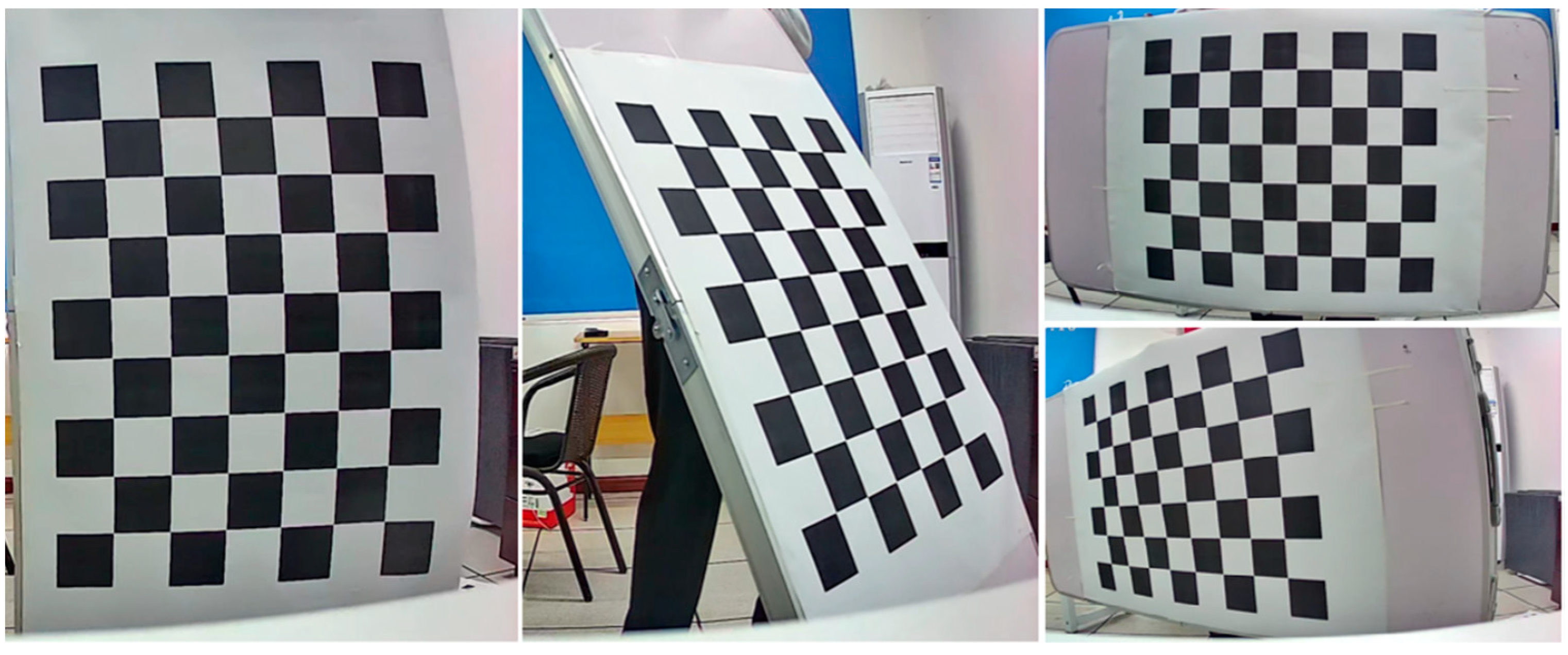
The intrinsic and extrinsic camera matrices were determined through Zhang’s calibration algorithm in MATLAB. According to this method, the intrinsic and extrinsic parameters of a camera can be estimated from several checkerboards taken at different orientations by the camera in question. In this way, the camera projection matrix can be estimated. While the intrinsic parameters do not change, the extrinsic parameters change with the change in camera position and orientation for side, front, and bottom views but are constant for any given validation since the camera is fixed. The camera used for image capturing was the HIKVISION wide-angle camera, the resolution of which is configured as 3024 × 4032.

An asymmetric checkerboard of high precision was adopted, where a total of 18 images shot at different orientations were collected and applied for calibration. Among them, four orientations are given, as in Figure 15 below. The intrinsic parameter matrix is estimated as in Equation (33).

$$\left[\begin{array}{ccc}\frac{f}{{\rho }_{\mathrm{w}}}& 0& u_0\\ 0& \frac{f}{{\rho }_{\mathrm{h}}}& v_0\\ 0& 0& 1\end{array}\right]=\left[\begin{array}{ccc}3271.91& 0& 1474.78\\ 0& 3273.81& 1992.86\\ 0& 0& 1\end{array}\right]$$

(33)

where f is the focal length, ρ_w and ρ_h are the width and height of each pixel, (u₀, v₀) is the principal point in pixels, i.e., the coordinate of the point where the optical axis intersects the image plane.

4.2. Image Processing Algorithm

The proposed model relies on the accurate detection of the coordinates of the endpoints of the stick to determine the varying slope in case of the front view, or the length, in case of other views.

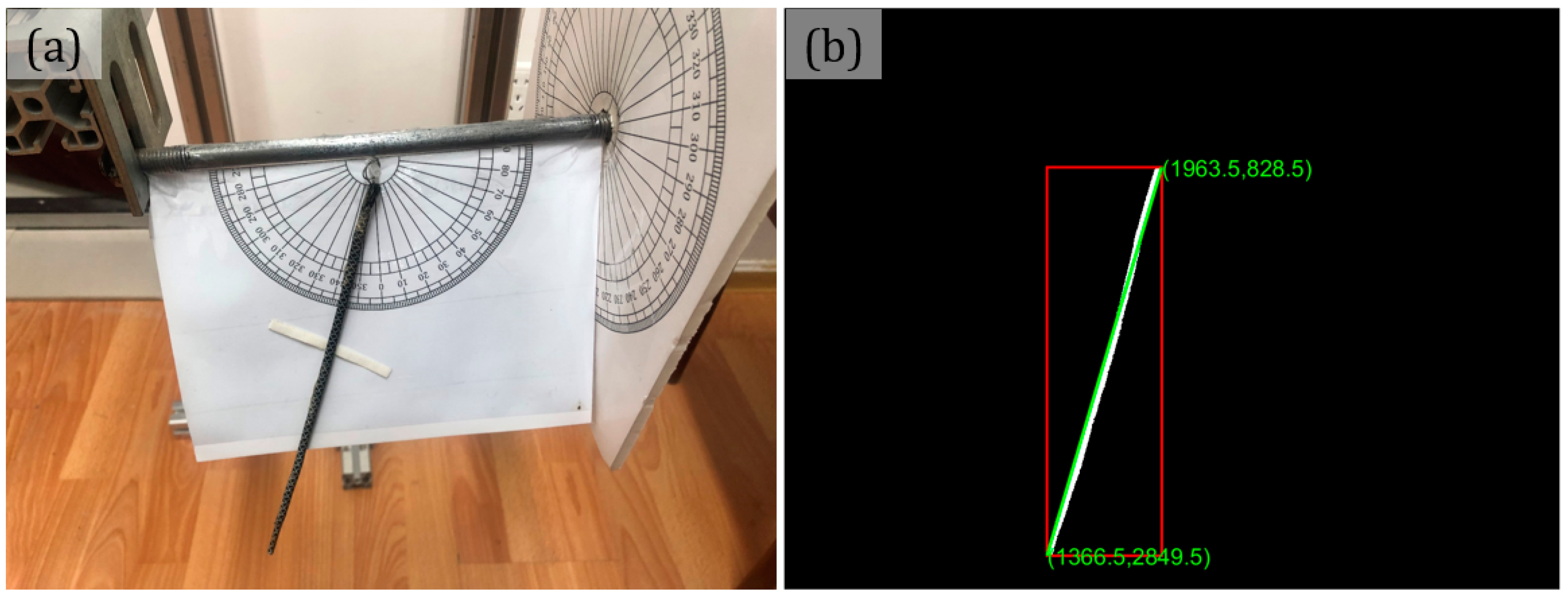
In the validation stage where only one image frame is required per test case, to determine the length and/or slope parameter(s), a standard object segmentation procedure [24] was written in MATLAB to separate the foreground (stick) from the background. After adjusting the intensity of the image to enhance the contrast of the Region of Interest (ROI), the image was binarized and appropriately cropped before morphological operations (dilation and erosion) were applied to eliminate the thinner protractor lines in the background. Thereafter, the segmented stick region (in white color) was contained in an axis-aligned minimum bounding box (in red color) whose diagonal cuts through the region and touches the edges, serving as the line (in green) whose end coordinates represent the detected line coordinates as shown in Figure 16 below.

4.3. Model Validation

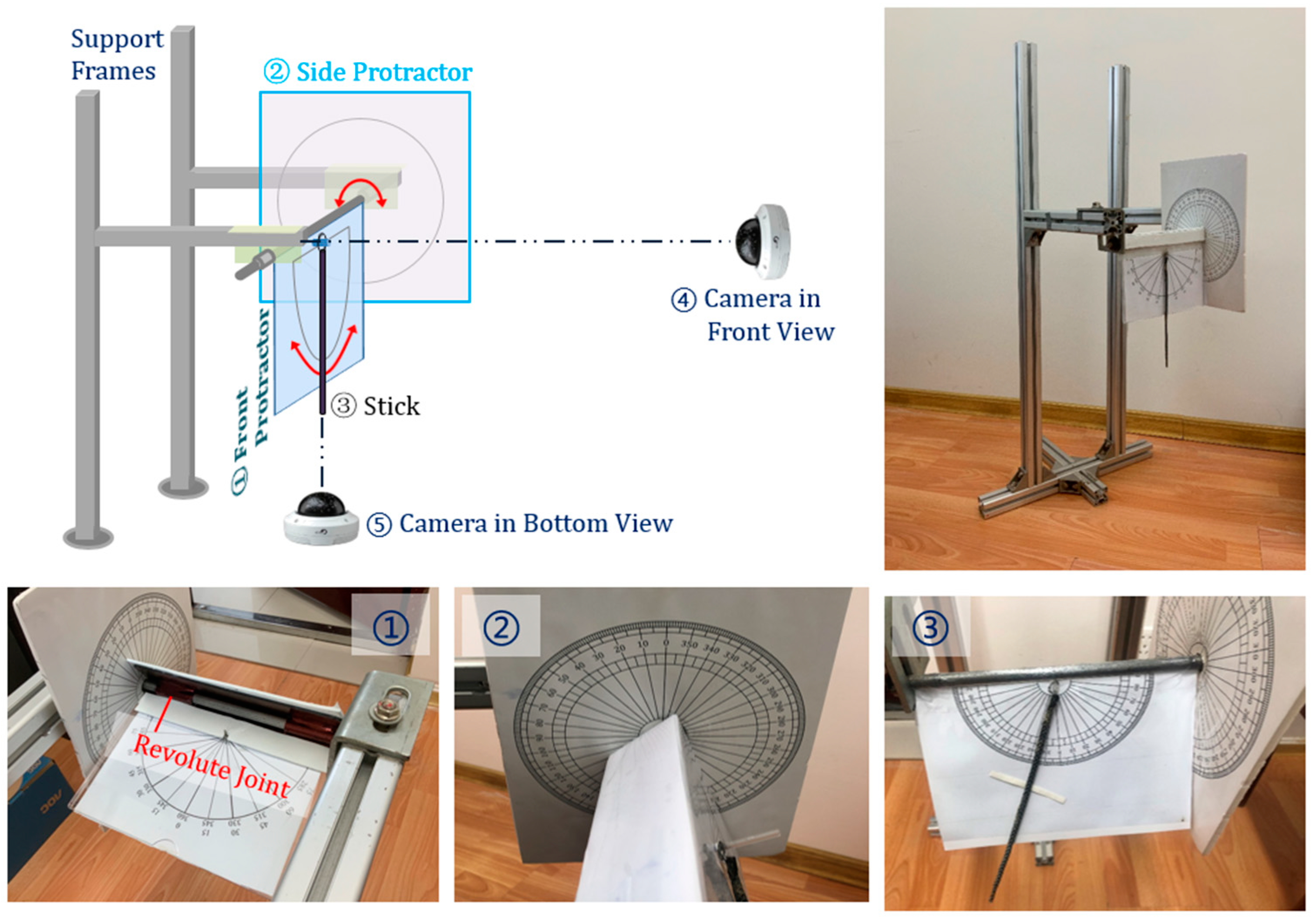
This section describes the implementation of the derived formulations through a validation experiment, where a system was set up as shown in Figure 17 below. The camera was employed in capturing the target’s displacement in bottom, side, and front views after swinging it in REV1# and/or REV2# direction(s) by a known magnitude with the aid of two protractors. Attached to the right and front sides of the cantilevered arm are the side and front plates on which the 360° and 180° protractors are placed, respectively. The front plate can be rotated (REV1#) up to 360° about the revolute joint, as in Figure 17 ①. The side plate is fixed and acts to perform the swing of the front plate in the REV1# direction, whereas the stick on the front protractor can be regulated in the swinging range of ±90° at REV2# by double-faced adhesive tape between the stick and the front protractor plate, as in Figure 17 ③.

The side and front protractors are designed to change the stick’s orientations. However, there is an indirect relationship between REV1#, REV2#, and the yaw angle, the wind direction angle. In the coupled imaging cases, given that the stick OA is first rotated in the front plate by α_Rev2# up to OA′ according to the front protractor, and the front plate is then rotated by α_Rev1# to a new position OA″ according to the side protractor, the two steps can be illustrated in Figure 18a below, in terms of a fan-shaped cylinder. When mathematically geometrized, the model can be expressed as a triangular prism in Figure 18b where ∠AOA′ describes the stick swing angle α_Rev2# in the front plate and ∠AOD denotes the front plate swing angle α_Rev1# along the side plate. Accordingly, the stick yaw angle α is the angle between the initial and ultimate position ∠AOC. The wind direction is the angle between △OAC and △OAD, denoted as α_WD, which is found by constructing a perpendicular plane between them.

In light of the stick length L, |OA| = |OD| = L. From the equivalent right triangles △ODC and △OAB, we can write:

|AB| = |CD| = L·tanα_Rev2#
|OC| = L/cosα_Rev2#

(34)

In △OAD, adopting the law of cosines:

$$|\mathrm{AD}{|}^2=|\mathrm{OA}{|}^2+|\mathrm{OD}{|}^2-2\cos {\mathsf{\alpha }}_{\mathrm{Rev}1\#}·|\mathrm{OA}|·|\mathrm{OD}|=2L^2·(1-\cos {\mathsf{\alpha }}_{\mathrm{Rev}1\#})$$

(35)

In the Rt△CDA, we have:

|AC|² = |CD|² + |AD|² = L²·(tan²α_Rev2# − 2cosα_Rev1# + 2)

(36)

In the △OAC, employing the law of cosines again based on (34) and (36) above, we have:

Cosα = (|OA|² + |OC|² − |AC|²)/(2|OA|·|OC|) = cosα_Rev1#·cosα_Rev2#

(37)

The yaw angle α is thus given in terms of REV1# and REV2# in Equation (37) as below.

α = cos⁻¹(cosα_Rev1#·cosα_Rev2#)

(38)

To find a joint perpendicular plane of both △OAC and △OAD, DF is created in △OAD and vertically intersects with OA at F. Since the face OABE rotates about OE to face ODCE, CD⊥△OAD, thus OA⊥CD. Since OA⊥DF, then OA⊥△CDF. Thus, any plane which has OA is perpendicular to △CDF, which means △OAC and △OAD are both perpendicular to △CDF. Therefore ∠CFD is the wind direction angle α_WD.

In △CDF, CD⊥DF because CD⊥△OAD. Thus, the wind direction is given as below.

$${\alpha }_{\mathrm{W}\mathrm{D}}={\mathrm{t}\mathrm{a}\mathrm{n}}^{-1}\left(\frac{\left|\mathrm{C}\mathrm{D}\right|}{\left|\mathrm{D}\mathrm{F}\right|}\right)={\mathrm{t}\mathrm{a}\mathrm{n}}^{-1}\left(\frac{\mathrm{t}\mathrm{a}\mathrm{n}{\alpha }_{\mathrm{R}\mathrm{e}\mathrm{v}2\#}}{\mathrm{s}\mathrm{i}\mathrm{n}{\alpha }_{\mathrm{R}\mathrm{e}\mathrm{v}1\#}}\right)$$

(39)

Hence, if rotated in both REV1# and REV2#, respectively, in front and side protractors, the practical stick yaw angle and wind direction are given in Equations (38) and (39), respectively. In this way, when the camera is placed in front as in Figure 17 ④ or at bottom as in Figure 17 ⑤, pure imaging cases, which only consider the yaw angle variation, can be simulated by changing REV1# as side view imaging cases, and REV2# as front view cases when the camera is placed in front. Accordingly, the pure bottom view case is simulated by changing REV1# when the camera is placed at bottom. Those cases will be included in Section 4.3.1—validation of pure imaging views. If REV1# and REV2# are coordinated at the same time to a certain amount of magnitude, the detected yaw angle and wind direction will be compared with theoretical ones in coupled bottom view and coupled side-front view.

4.3.1. Validation of Pure View Cases

In validation tests of pure imaging views, camera parameters are given in

Table 2. Camera parameters.

Parameter	Deviated Bottom View	Deviated Side View	Deviated Front View
Stick length L (mm/px)	225/1101	225/1238	225/1238
Object distance DO (mm/px)	670/3279	600/3301	600/3301
Deviation S (mm/px)	70.4/344	68.7/387	68.7/387
Focal length f (px)	3273	3273	3273
Camera resolution (px)	3024 × 4032	3024 × 4032	3024 × 4032

Note: ‘px’ denotes unit ‘pixel’.

including the stick length, object distance, optical deviation, focal length, and camera resolution in bottom, side, and front views. Among them, the camera is placed at a deviation of 70.4 mm and 68.7 mm, respectively, in bottom and side view. In front view, the camera is placed at the same position as in side view case. However, the stick is adjusted by only REV2# in the front plate.

In pure deviated bottom view, the stick lines are in its initial vertical direction in the front plate. The plate is rotated by REV1# in the range of ±90° at an interval of 15°. Imaging length X_P is calculated by identifying the pixel coordinates of the fixed and free stick ends, which are then substituted into Equation (6) to acquire the yaw angle α at each REV1# case. To better compare and validate the test results, two continuous curves are given for the proposed detection model by obtaining the imaging length X_P from the discretized yaw angle α (0.5° interval) based on Equation (5) as the dashed red line, and also by acquiring the yaw angle α from the above discretized imaging length X_P based on Equation (6) as the blue solid line in Figure 19 below. Left and right limit angles are computed according to Equations (10) and (11), and depicted as the two horizontal lines; the top 77.6° describes the left and the bottom −83.2° denotes the right limit angle. The 13 detected yaw angles are illustrated as circular, blue-edge markers which go well with the detection model, while the red markers are the results beyond the limit.

From the above, it is seen that when the yaw angle cases vary between the left and right angle limits, the detected yaw angles agree well with the theoretical detection model (Equation (6)). However, when REV1# is ±90° beyond the limit of −83.2 to 77.6°, there is a big deviation between the detected and the expected, as shown in the red circular markers. Due to the geometrical relationship, the detected and the expected yaw angles are symmetric to the left and right limits, respectively, for 90° and −90° yaw angle cases.

In pure deviated side view, the camera is placed in front of the front plate, but the stick stays at the same position while the front plate is rotated in the same way as in the bottom view cases. The identified imaging length X_P is substituted into Equation (18) to acquire the yaw angle α at each REV1# case. The left and right limits are calculated as 90° and −13.0° according to Equation (22) and Equation (23). The detection model from yaw angle to imaging length, and the inversion model, are respectively denoted as the dashed red line and solid blue line in Figure 20. Detected yaw angles in 13 REV1# imaging cases are illustrated as circular blue-edge markers, among which the red markers indicate the results that are beyond the limit.

It can be observed that when the REV1# imaging cases vary between 90° and −13.0°, the detected yaw angles agree well with the theoretical detection model (Equation (18)). However, when REV1# is below the right limit of −13.0°, there is a big deviation between the detected and the expected as shown in the red circular markers. As REV1# increases in the negative direction, the difference becomes bigger. Due to the same geometry rules however, the detected yaw angles placed over the blue solid line—the detection model—are symmetrical to the right limit angle with the expected yaw angles on the red dashed line beyond the limit (Figure 20).

In pure deviated front view, the camera is placed in the same position as in the deviated side view, whereas the front plate remains still, and the stick is rotated by REV2# in the range of ±90° at an interval of 15°. Pixel coordinates of the stick’s ends are identified and substituted into Equation (24) to obtain the yaw angle α within its physical limits. From the above, the detected yaw angles as well as their corresponding imaging lengths in bottom and side view cases, and identified slopes in front view cases, are listed in

Table 3. Validation results of pure imaging tests in bottom, side, and front views.

Given Yaw Angle /°	Bottom View		Side View		Front View
	Imaging Length (px)	Detected Angle (°)	Imaging Length (px)	Detected Angle (°)	Identified Slope	Detected Angle (°)
−90	−550.1	−76.8	40.2	81.6	−381.9671	−89.9
−75	−544.5	−73.2	201.4	61.6	−3.8118	−75.3
−60	−497.5	−58.5	357.2	40.5	−1.7689	−60.5
−45	−425.4	−46.1	463.5	22.4	−0.9752	−44.3
−30	−301.9	−30.9	532.8	5.8	−0.5973	−30.8
−15	−147.5	−15.8	562.1	−10.7	−0.2867	−16.0
0	33.5	−0.1	544.8	1.4	−0.0204	−1.2
15	197.9	14.5	504.7	13.8	0.2467	13.9
30	359.7	30.8	417.6	30.8	0.5539	29.0
45	477.7	46.2	329.9	44.3	0.9715	44.2
60	538.9	61.1	218.8	59.5	1.6888	59.4
75	562.1	73.3	91.2	75.5	3.6584	74.7
90	549.8	65.1	−23.5	89.4	381.9671	89.9

Note: ‘px’ denotes ‘pixel’.

below. The error between the detected and given yaw angles is plotted in Figure 21.

It is seen that in the deviated side view case, the absolute error between the detected and expected yaw angle varies within 1.5° in the range of −13.0 to 90°. However, as the given yaw angle negatively increases beyond the detection limit, the error grows from 4.3° to as high as 171.6° because of its incapability in identifying the imaging length change in the stick when approaching or going away from the camera. In deviated bottom view, the error is within 1.8° when the given yaw angle changes in the limit range, whereas it rises to 13.2° and 24.9° at ±90° beyond the angle limit. Among all imaging views, the front view attains the best performance in its yaw angle detection precision due to the slope-only dependent measurement of the stick image, where the maximum error is no more than 1.2°. It is therefore recommended that coupled view with front-dominated detection be employed in practical application.

4.3.2. Validation of Coupled View Cases

In coupled view imaging cases, the camera is placed at bottom and in front of the front plate, just as in the bottom-front coupled view and side-front coupled view cases where the yaw angles and wind directions are both regulated. For different coupled view cases, the practical yaw angle and wind direction are simulated by adjusting REV1# in the range of 0 to 90° and REV2# in the range of ±90°, in steps of 15°. In each imaging case, the yaw angle and wind direction are calculated according to Equations (38) and (39) based on the given REV1# and REV2#.

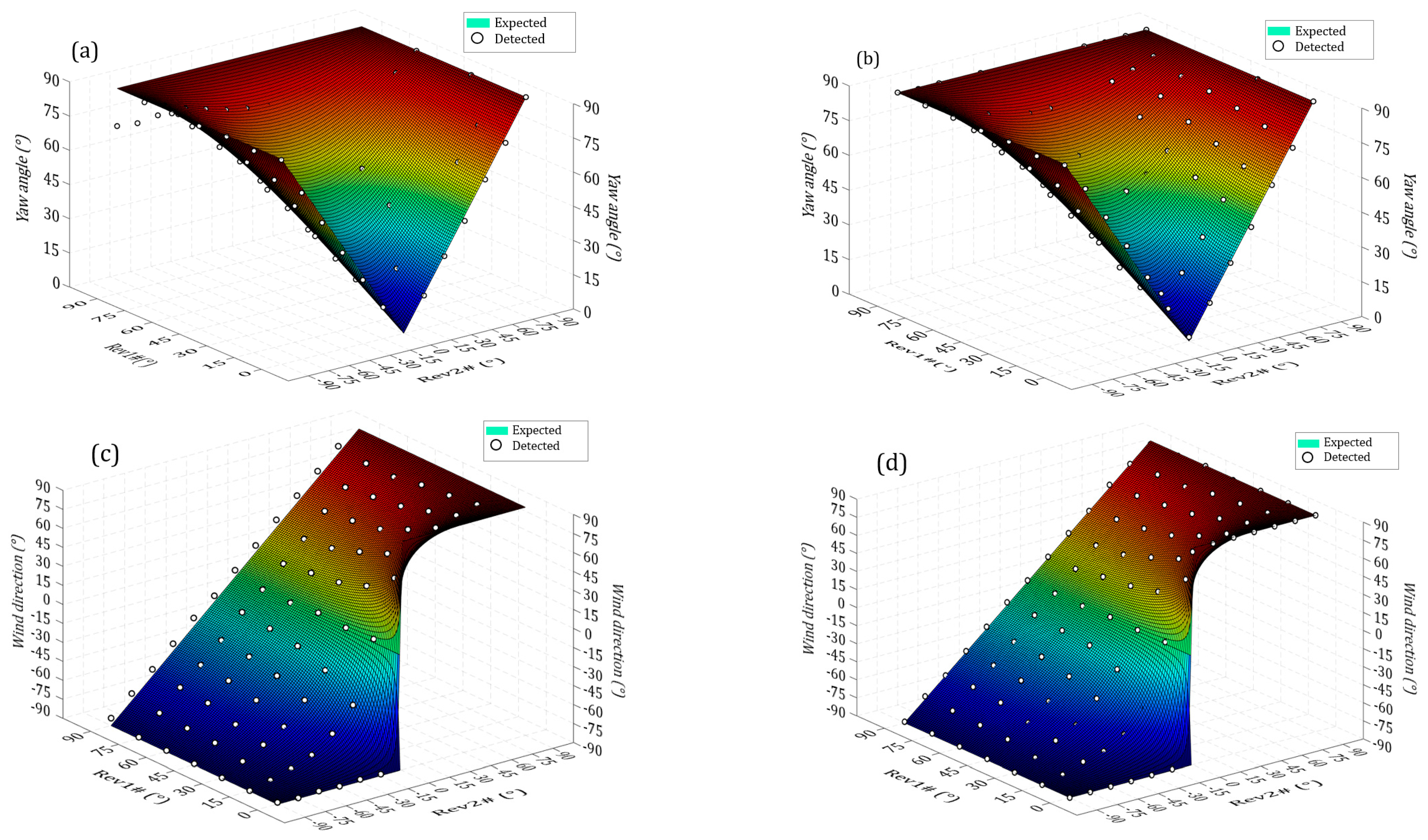
The camera is fixed in the same position as in the pure deviated bottom view, for bottom-front coupled view imaging case, and as in the pure deviated side view, for the side-front coupled view imaging case. Detected yaw angles and wind directions are calculated based on the stick’s imaging length and orientation, respectively, according to Equations (6) and (12) for bottom-front coupled view, and according to Equations (27) and (28) for side-front coupled view. 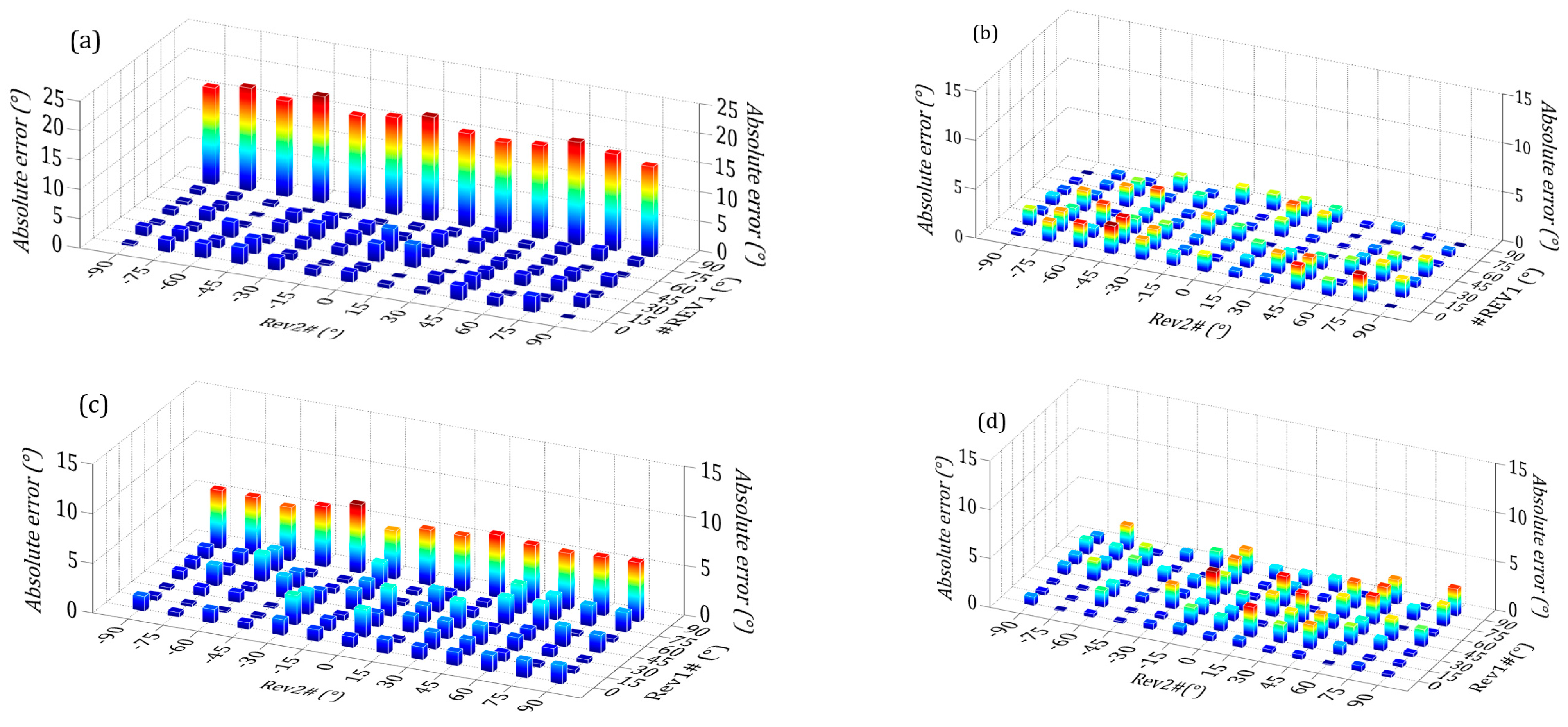The detected results are denoted as black-edged white circles and compared with the 3-D contour curve surface of the expected yaw angle and wind direction acquired from REV1# and REV2# in a dense space of 0.5°, as shown in Figure 22a, 21b, 21c, 21d, respectively, for yaw angle detection in bottom-front and side-front coupled view, and wind direction detection in bottom-front and side-front coupled view. The absolute errors between detected and expected results are accordingly given in terms of 3-D contoured bars in Figure 23a, 22b, 22c, 22d, respectively, for the above cases.

It can be observed that all the detected results agree well with the expected cases, both in terms of yaw angle and wind direction detections, as depicted in the 3-D surface plots. The maximum absolute error for yaw angle detections is 4.0° within the limit range and climbs to 18.1° beyond the limit in bottom-front coupled view, compared to a smaller maximum absolute error of 2.9° in side-front coupled view validation. This is because the validated yaw angle range in side-front coupled view covers all validated cases, whereas in bottom-front coupled view, it exceeds the limit range above the 75°. In wind direction detection, a similar trend is seen as in bottom-front coupled view where the maximum absolute error is no more than 3.0° within the limit range but climbs to 5.9° above the limit. The maximum error is 3.4° for side-front coupled view, which is proximal to the bottom-front view within its yaw angle limit range. In all, the results show that the proposed method measures both yaw angle and wind direction with good accuracy, provided that the limit range of measurement is not exceeded.

5. Practical Application

5.1. Test Overview

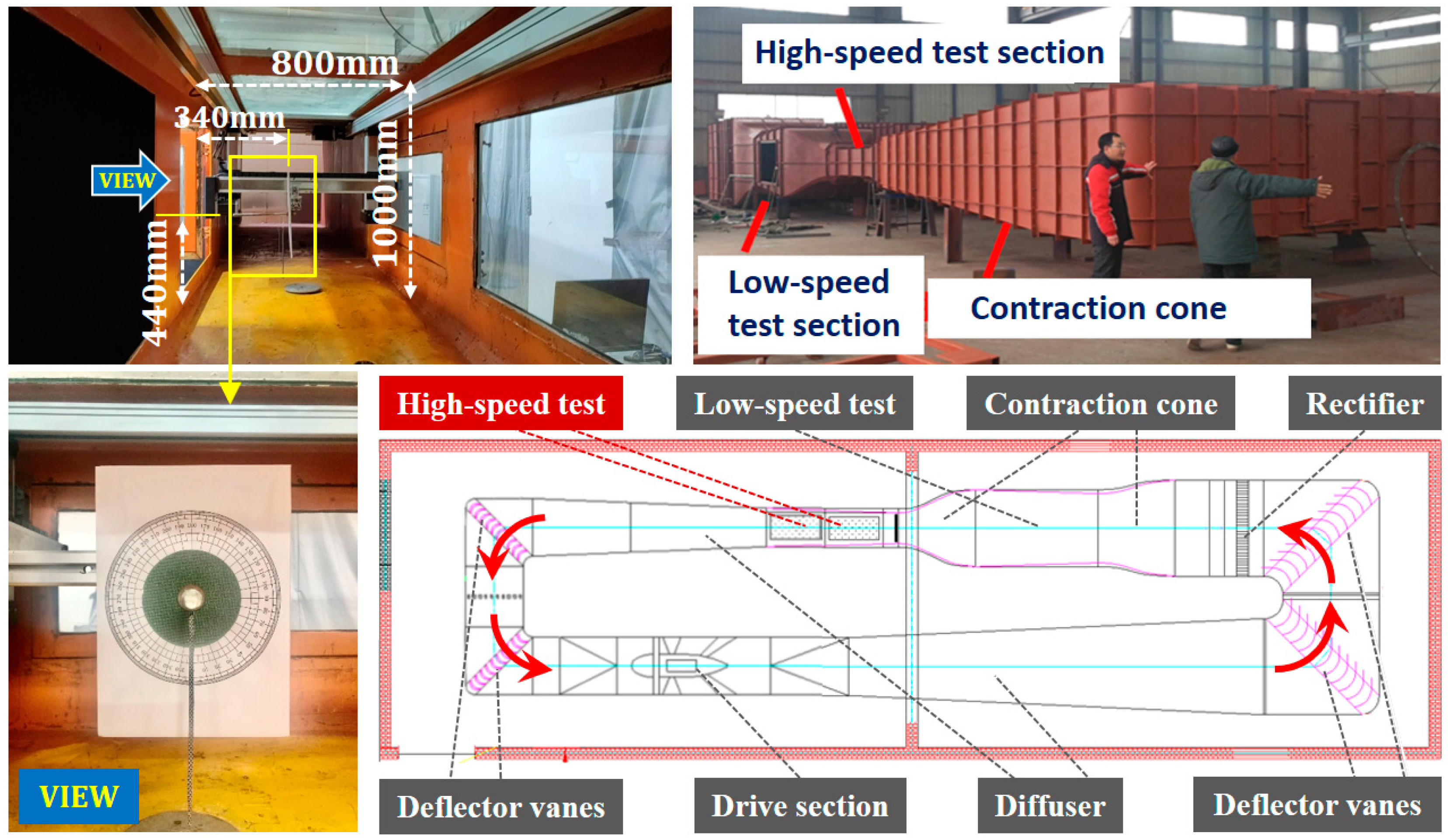
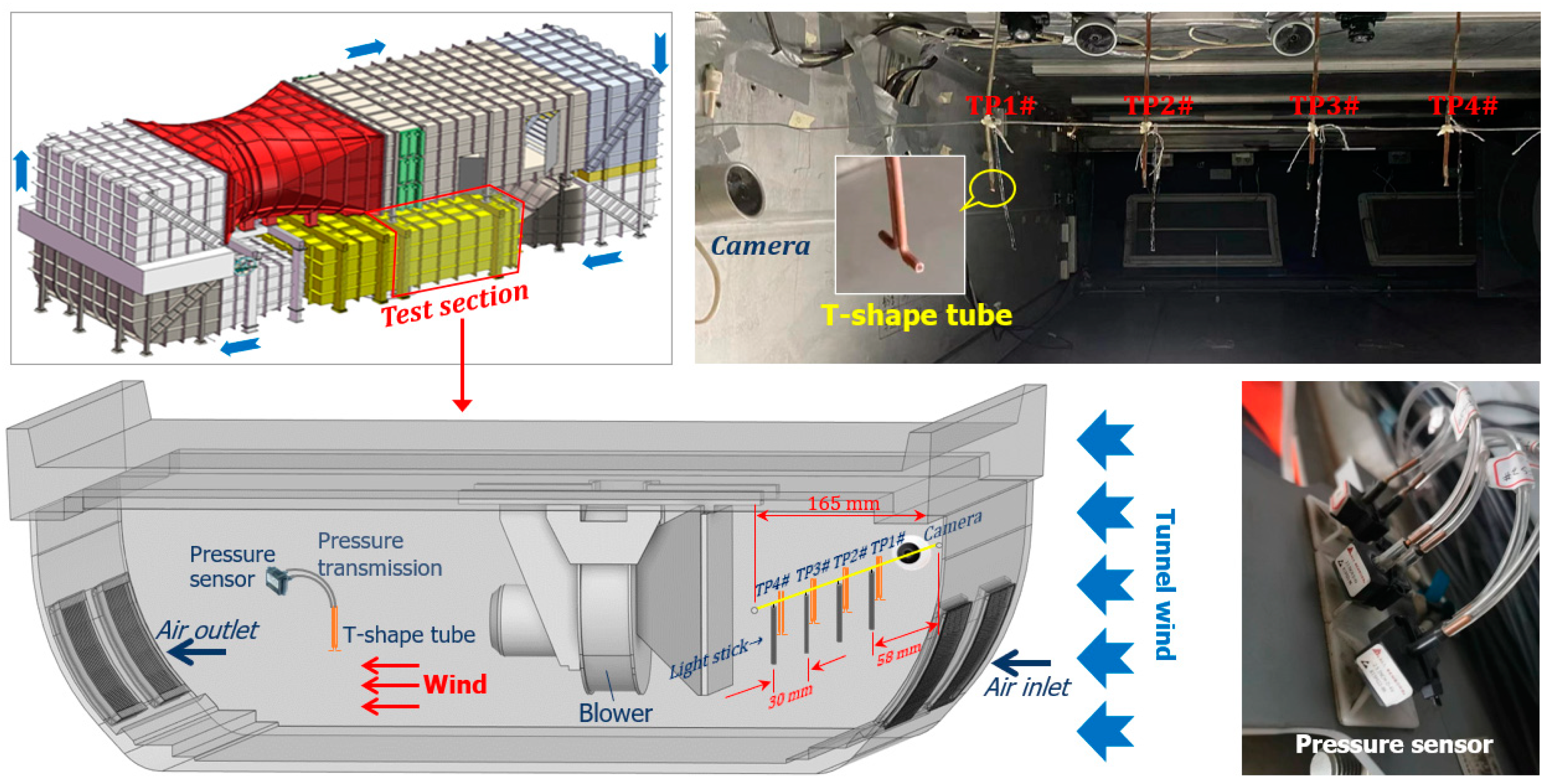
To demonstrate the applicability of the proposed method in practical cases, a wind tunnel test was implemented in the stationary equipment cabin of a high-speed train. Unlike the wind tunnel calibration test in Section 3.2, the Environmental Wind Tunnel (EWT) is a vertical closed circuit with an open test section (4 m × 1 m at the inlet and 6.7 m in length). The key components of the wind tunnel consist of insulation layers, axial fan, and the rotary table with wheelset drive system, etc.

In the wind tunnel test, the cabin was situated in the test section with its air inlet facing the tunnel airflow direction where filter screens are installed behind the inlet grills at the skirt plate to prevent dust accumulation in the cabin. Since the air filter can influence the flow characteristics inside the compartment, four 225 mm long light sticks were equally spaced at 30 mm, and aligned 165 mm away from the inlet grills, in an attempt to detect the wind speed behind the grills and air filters. This is also important to test the uniformity of the flow at different points with the same camera. Four T-shape tubes were fixed beside each stick and linked with a pressure transmission pipe to pressure sensors to test the wind speed based on the pitot method as the reference for the proposed method. Finally, a video camera was placed 58 mm away from the closest stick on the cabin wall in a side-front coupled view to observe the yaw angle of the four light sticks, the location of which are respectively denoted as TP1#, TP2#, TP3# and TP4#, shown in Figure 24. The camera has the same parameters as in the model validation section. Image sequences of the stick motion and corresponding wind pressure were simultaneously measured respectively by the camera and pitot T-tube. Thereafter, a video processing algorithm was implemented in MATLAB to identify each moving stick and determine their respective angular displacements.

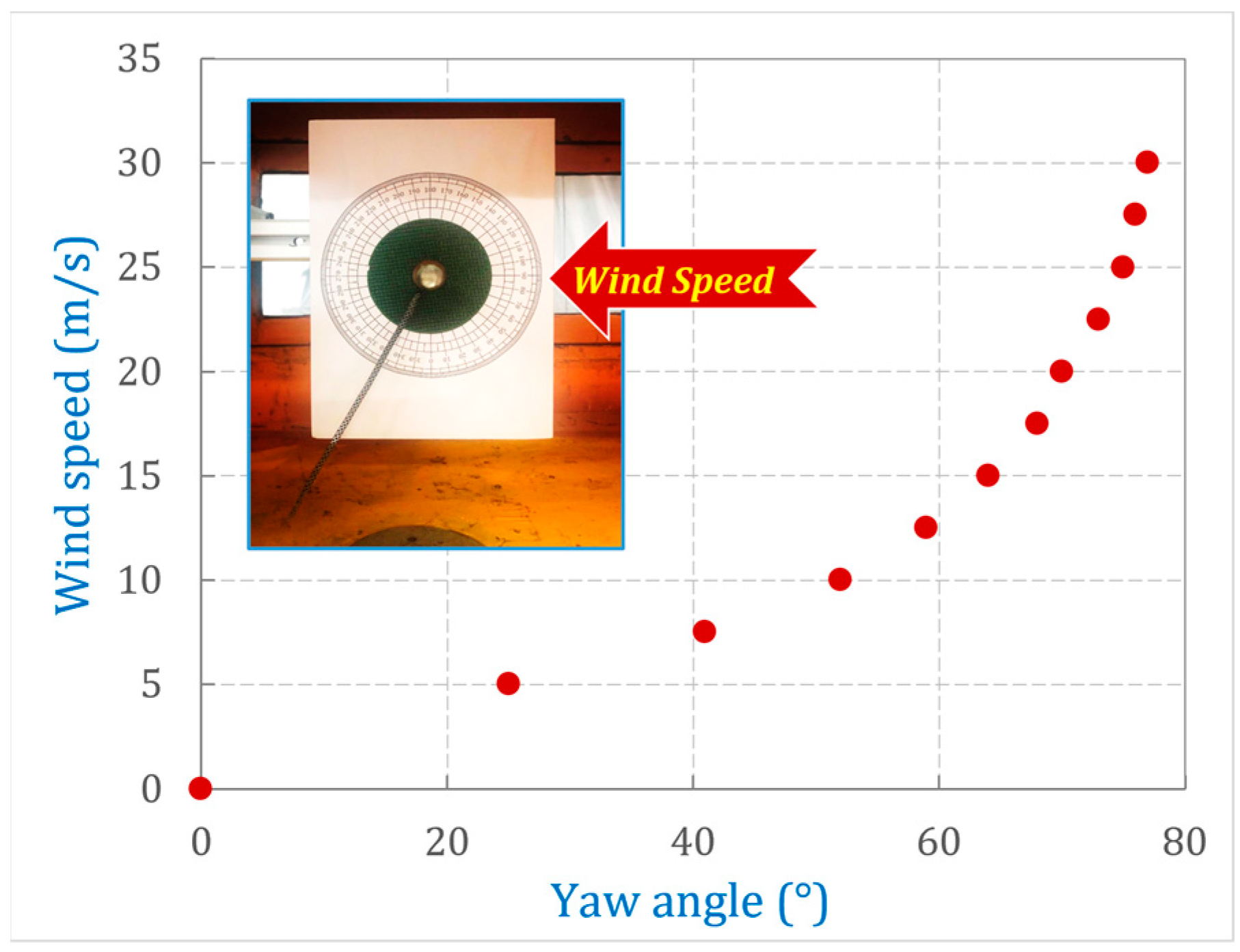
In the experiment, five wind tunnel speed cases were set from 0 m/s to 25 m/s at intervals of 5 m/s. When the tunnel wind is 0 m/s, the detected wind speed is the wind flow from the external environment driven by the blower inside the cabin. During the 6 tunnel wind stages, the motion of light sticks was recorded and extracted into 24 image frames per second to acquire the time history of their yaw angle variations. Dynamic pressures of the pitot T-tube were collected by IMC DAQ system at a sampling frequency of 256 Hz. The dynamic pressure data were processed with low-pass filtering at a frequency of 40 Hz, and then used to determine the corresponding wind speed data according to the Bernoulli equation:

$$v_{\mathrm{c}}=\sqrt{2\rho ·P_{\mathrm{d}}}$$

(40)

where $v_{\mathrm{c}}$ is the wind speed (m/s), $P_{\mathrm{d}}$ is the dynamic pressure (Pa), and $\rho$ is the atmospheric density, 1.225 kg/m³.

5.2. Results and Discussion

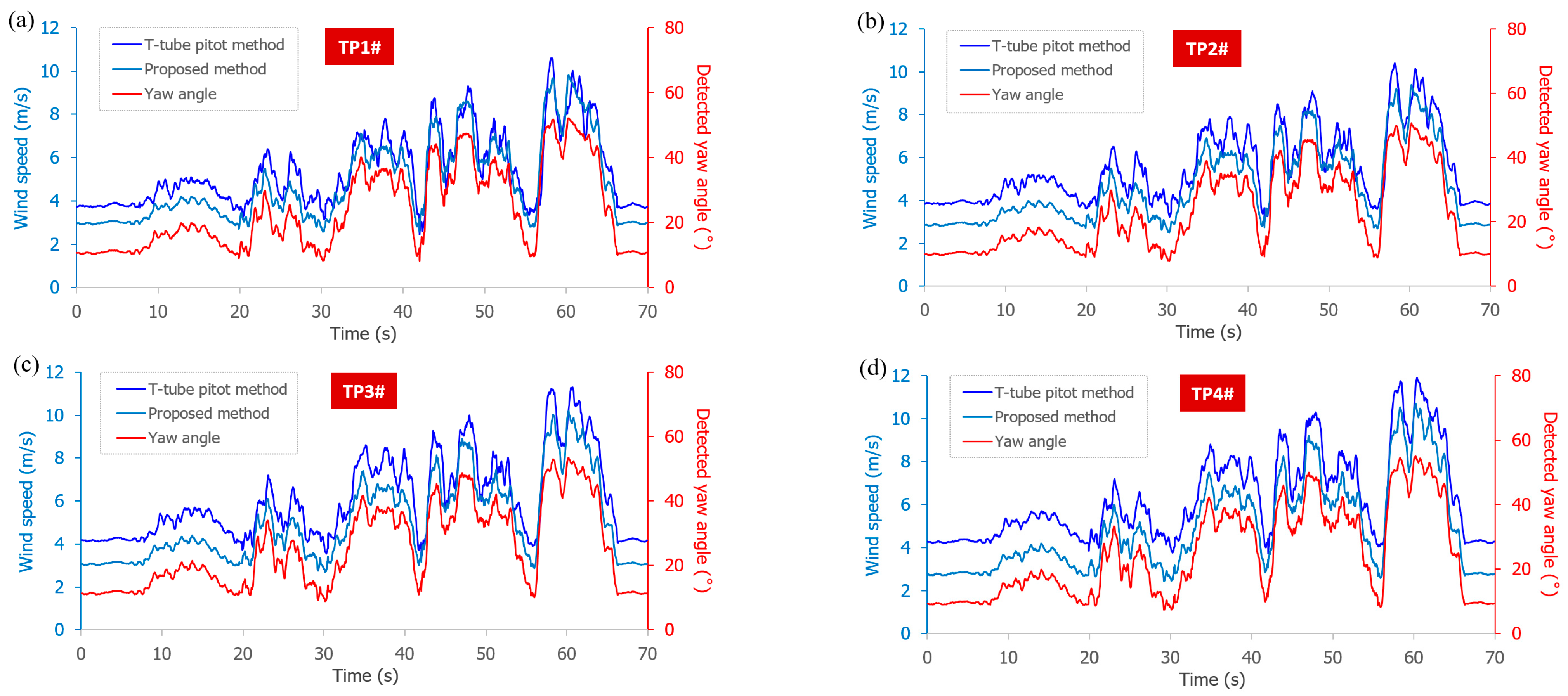
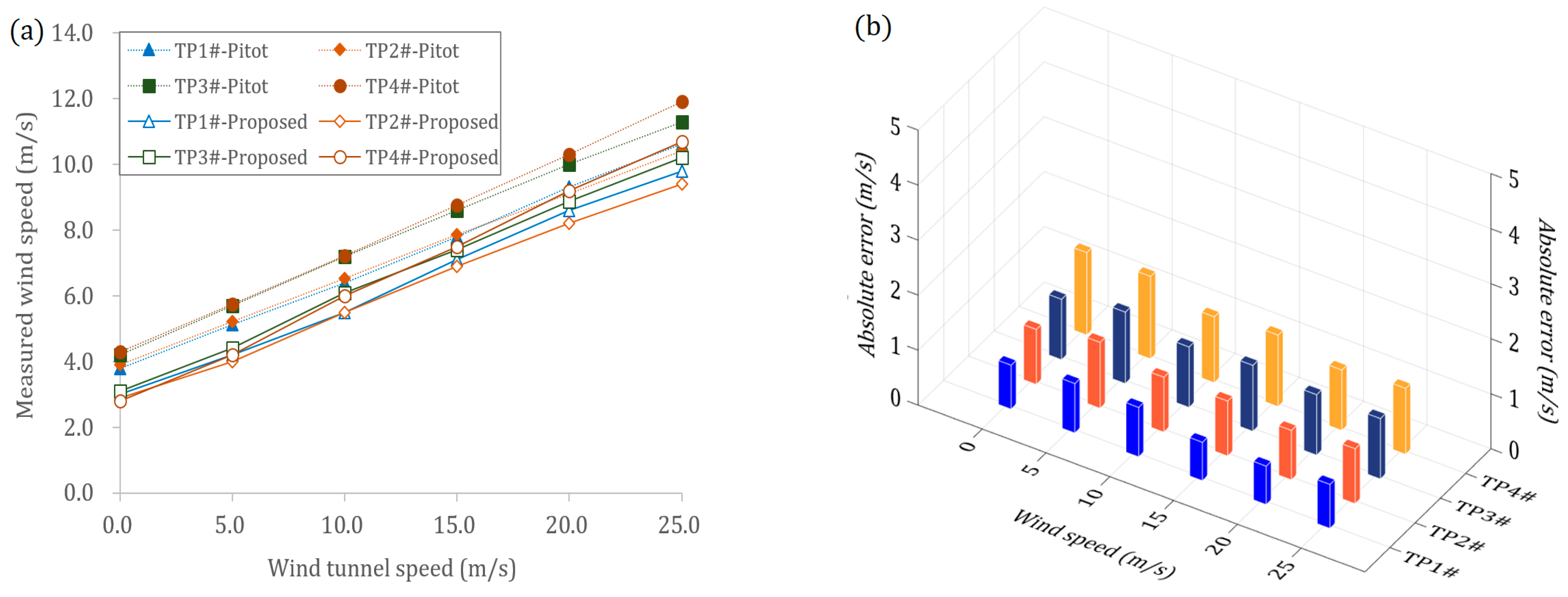
The detected yaw angles of the light sticks, the corresponding calculated wind speeds, and the measured wind speed based on the T-tube pitot method at the four test points TP1#, TP2#, TP3#, and TP4# are given in terms of time-history curves (Figure 25). Encouraging agreement is observed in the variation trend between the proposed method and the T-tube pitot method.

As seen above, during the first 8 s when no wind is blowing in the tunnel, the sticks stay in a constant yaw angle due to the steady flow driven by the inner blower from the outside environment. When the tunnel wind increases to 5 m/s, 10 m/s, 15 m/s, 20 m/s, and 25 m/s, the sticks displace to-and-fro, accordingly, with good response to prevailing wind fluctuation detected by the T-tube pitot. However, wind speed detection via the proposed method is smaller than that detected by the T-tube pitot method and there is also a slight time delay in the peak response of the proposed method. Because the motion of the stick is mainly influenced by the interplay between its deadweight, gravity, and wind pressure, as the wind speed increases, the response time also generally climbs because it takes longer for the stick to find a new equilibrium state from a higher starting speed, as gravity forces it to return. Furthermore, in general, the stick rises almost steadily from the first instance of a speed increase, fluctuates around the peak speed for the same equilibrium-finding reason, before it falls at the end of the test case. At every increase in wind speed, the stick rises almost steadily, which can also be observed in the pitot measurement. The T-tube method also appears to be more sensitive to sharp variations in the wind speed. While the proposed method follows the trend closely, it does not capture the peaks as sharply because, for some split-second, it needs to rise or fall, while continually pushing towards an equilibrium state that continues to change. In contrast, the T-tube pitot method has no moving parts and so directly senses the pressure as it varies over time.

In addition, and as is evident from the yaw angle trend, increasing and decreasing according to the prevailing wind speed, measurement beyond critical angle limits did not arise since the model adopted was front-view dominated where limits are $\pm 90°$ (Equation (25)), which is the maximum.

By calculating the absolute error between values detected by the proposed method and those expected by the T-tube pitot at each test point, the Root Mean Square Errors (RMSEs) are ±0.8 m/s, ±1.01 m/s, ±1.2 m/s, and ±1.4 m/s, respectively, for TP1#, TP2#, TP3#, and TP4# (Figure 26) when the maximum yaw angles are detected at 52.1°, 50.7°, 53.5°, and 55.1°. The two methods agree well, although the proposed method is offset lower by about 0.73 m/s on average from the T-tube pitot method. This offset may be due to the inaccurate estimation of the T-tube pitot orientation [25,26].

The results comparison between the two methods at the four test points shows a mean absolute error of 1.1 m/s. The imperfectly uniform distribution of wind pressure, inaccurate estimation of the T-tube pitot orientation, and image-processing-related errors are suspected to account for the relative differences in the measurement results seen at the different test points. The low RMSE values demonstrate the robustness of the proposed method to measure wind speed with good response time.

6. Conclusions and Outlook

In this work, a novel wind speed measurement methodology is proposed by visually identifying the wind-induced motion of lightweight sticks. The presented model is validated by a designed simulation set-up for a theoretical model and applied in wind tunnel tests in a stationary inner equipment cabin of a high-speed train. The conclusions derived are as follows:

(1) Imaging models are given between the yaw angle, wind direction, and imaging length, as well as the orientation of the light stick target, when the camera is respectively placed at its bottom, side, and front, in pure and coupled imaging views. The models were validated by using a simulation set-up with multiple revolute joints to acquire different yaw angle and wind direction cases, in which the maximum error is no more than 3.4°.

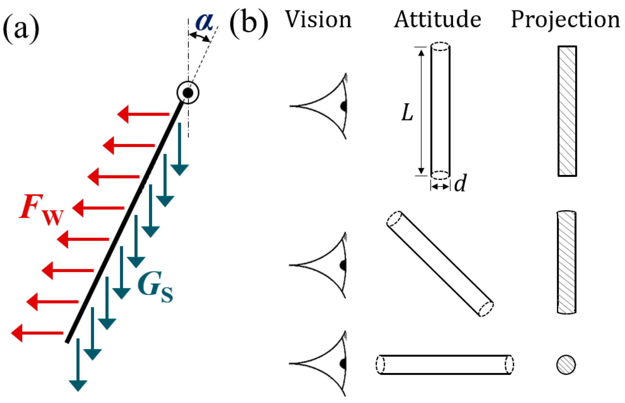
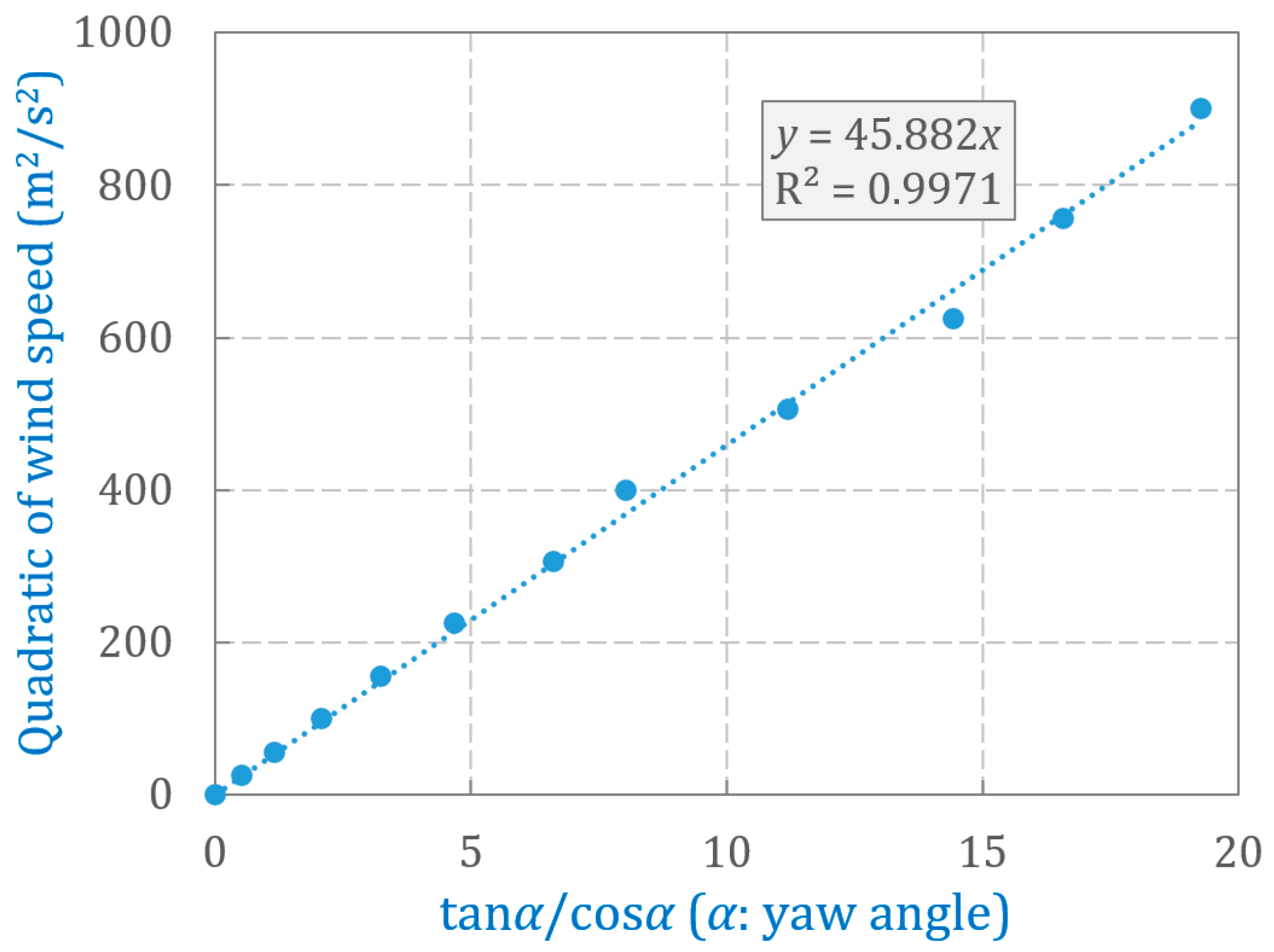
(2) The mathematical relationship between the stick yaw angle and the wind speed was calibrated through wind tunnel tests, where a linear relationship was observed between the quadratic power of the wind speed and the compound trigonometric function of the yaw angle. The derived relationship is also explained by a mechanical formulation based on the force equilibrium of a hanging stick subjected to wind pressure and its gravity force.

(3) In the application of wind speed measurement in the limited space of an inner equipment cabin of a high-speed train, the proposed method shows good agreement with T-tube pitot detections. The error is no bigger than ±1.1 m/s in average RMSE at all test points in wind tunnel tests compared to the standard T-tube pitot readings, which indicates that the developed method provides an accurate and economic option for monitoring 2-D wind speed in a confined space.

(4) Future work will focus on addressing the vertical wind speed component that will affect the stick yaw angle detection, by adding more information besides the yaw angle and projection length of the stick. We will also work on grouping different light sticks by relating their geometry and mechanical parameters with the wind speed measurement range to accommodate more complex application circumstances.

References

1. Patel, R.; Patel, S. A comprehensive study of applying convolutional neural network for computer vision. Int. J. Adv. Sci. Technol. 2020, 6, 2161–2174. [Google Scholar]
2. Kitahara, T.; Satou, K.; Onodera, J. Marking robot in cooperation with three-dimensional measuring instruments. In Proceedings of the ISARC, International Symposium on Automation and Robotics in Construction, Berlin, Germany, 20–25 July 2018; Volume 35, pp. 1–8. [Google Scholar]
3. Janai, J.; Güney, F.; Behl, A.; Geiger, A. Computer vision for autonomous vehicles: Problems, datasets and state of the art. Found. Trends® Comput. Graph. Vis. 2020, 12, 1–308. [Google Scholar] [CrossRef]
4. Hanlon, T.; Risk, D. Using computational fluid dynamics and field experiments to improve vehicle-based wind measurements for environmental monitoring. Atmos. Meas. Tech. 2020, 13, 191–203. [Google Scholar] [CrossRef] [Green Version]
5. Tran, M.Q.; Li, Y.C.; Lan, C.Y.; Liu, M.K. Wind Farm Fault Detection by Monitoring Wind Speed in the Wake Region. Energies 2020, 13, 6559. [Google Scholar] [CrossRef]
6. Ritvanen, J.; O’Connor, E.; Moisseev, D.; Lehtinen, R.; Tyynelä, J.; Thobois, L. Complementarity of wind measurements from co-located X-band weather radar and Doppler lidar. Atmos. Meas. Tech. 2022, 15, 6507–6519. [Google Scholar] [CrossRef]
7. Clifton, A.; Barber, S.; Stökl, A.; Frank, H.; Karlsson, T. Research challenges and needs for the deployment of wind energy in hilly and mountainous regions. Wind Energy Sci. 2022, 7, 2231–2254. [Google Scholar] [CrossRef]
8. Kogaki, T.; Sakurai, K.; Shimada, S.; Kawabata, H.; Otake, Y.; Kondo, K.; Fujita, E. Field measurements of wind characteristics using LiDAR on a wind farm with downwind turbines installed in a complex terrain region. Energies 2020, 13, 5135. [Google Scholar] [CrossRef]
9. Kim, D.Y.; Kim, Y.H.; Kim, B.S. Changes in wind turbine power characteristics and annual energy production due to atmospheric stability, turbulence intensity, and wind shear. Energy 2021, 214, 119051. [Google Scholar] [CrossRef]
10. Kumar, S.; Huang, R.F.; Hsu, C.M. Effects of pulsation intensity on the flow and dispersion of pulsed dual plane jets. Int. J. Mech. Sci. 2021, 193, 106182. [Google Scholar] [CrossRef]
11. Ariante, G.; Ponte, S.; Papa, U.; Del Core, G. Estimation of airspeed, angle of attack, and sideslip for small unmanned aerial vehicles (UAVs) using a micro-pitot tube. Electronics 2021, 10, 2325. [Google Scholar] [CrossRef]
12. Zhao, Y. Application of Computer-based Machine Vision Measurement System in Industrial On-line Detection. J. Phys. Conf. Ser. 2021, 1992, 022062. [Google Scholar] [CrossRef]
13. Yao, S.; Li, H.; Pang, S.; Zhu, B.; Zhang, X.; Fatikow, S. A Review of Computer Microvision-Based Precision Motion Measurement: Principles, Characteristics, and Applications. IEEE Trans. Instrum. Meas. 2021, 71, 5007928. [Google Scholar] [CrossRef]
14. Foken, T.; Bange, J. Wind Sensors BT—Springer Handbook of Atmospheric Measurements; Foken, T., Ed.; Springer International Publishing: Cham, Switzerland, 2021; pp. 243–272. [Google Scholar]
15. Alfonso-Corcuera, D.; Ogueta-Gutiérrez, M.; Fernández-Soler, A.; González-Bárcena, D.; Pindado, S. Measuring Relative Wind Speeds in Stratospheric Balloons with Cup Anemometers: The TASEC-Lab Mission. Sensors 2022, 22, 5575. [Google Scholar] [CrossRef] [PubMed]
16. Guerrero-Villar, F.; Dorado-Vicente, R.; Medina-Sánchez, G.; Torres-Jiménez, E. Alternative Calibration of Cup Anemometers: A Way to Reduce the Uncertainty of Wind Power Density Estimation. Sensors 2019, 19, 2029. [Google Scholar] [CrossRef] [Green Version]
17. Cui, C.; Cai, W.; Chen, H. Airflow measurements using averaging Pitot tube under restricted conditions. Build. Environ. 2018, 139, 17–26. [Google Scholar] [CrossRef]
18. Wei, M.; Zeng, Y.; Wen, C.; Liu, X.; Li, C.; Xu, S. Comparison of MCM and GUM method for evaluating measurement uncertainty of wind speed by pitot tube. MAPAN 2019, 34, 345–355. [Google Scholar] [CrossRef]
19. Cardona, J.; Howland, M.; Dabiri, J. Seeing the wind: Visual wind speed prediction with a coupled convolutional and recurrent neural network. In Advances in Neural Information Processing Systems 32 (NeurIPS 2019); Curran Associates, Inc.: New York, NY, USA, 2021. [Google Scholar] [CrossRef]
20. Yang, D.; Pan, Z.; Cao, Y.; Wang, Y.; Lai, X.; Yang, J.; Liu, Y. Wind measurement by computer vision on unmanned sailboat. Int. J. Intell. Robot. Appl. 2021, 5, 252–263. [Google Scholar] [CrossRef]
21. Ehsan, M.A.; Shahirinia, A.; Zhang, N.; Oladunni, T. Wind speed prediction and visualization using long short-term memory networks (LSTM). In Proceedings of the 2020 10th International Conference on Information Science and Technology (ICIST), Bath, London, and Plymouth, UK, 9–15 September 2020; pp. 234–240. [Google Scholar]
22. Gunnlaugsson, H.P.; Holstein-Rathlou, C.; Merrison, J.P.; Knak, J.S.; Lange, C.F.; Larsen, S.E.; Madsen, M.B.; Nørnberg, P.; Bechtold, H.; Hald, E.; et al. Telltale wind indicator for the Mars Phoenix lander. J. Geophys. Res. Planets 2008, 113, 2–7. [Google Scholar] [CrossRef] [Green Version]
23. Huo, J.; Zhang, H.; Meng, Z.; Yang, F.; Yang, G. A flexible calibration method based on small planar target for defocused cameras. Opt. Lasers Eng. 2022, 157, 107125. [Google Scholar] [CrossRef]
24. Pare, S.; Kumar, A.; Singh, G.K.; Bajaj, V. Image segmentation using multilevel thresholding: A research review. Iran. J. Sci. Technol. Trans. Electr. Eng. 2020, 44, 1–29. [Google Scholar] [CrossRef]
25. Petersen, M.; Larsen, T.; Madsen, H.; Larsen, G.; Toldborg, N. Turbulent wind field characterization and re-generation based on Pitot tube measurements mounted on a wind turbine. In Proceedings of the 33rd Wind Energy Symposium, Kissimmee, FL, USA, 5–9 January 2015. [Google Scholar]
26. Petersen, M.; Larsen, T.; Madsen, H.; Larsen, G. Using wind speed from a blade-mounted flow sensor for power and load assessment on modern wind turbines. Wind Energy Sci. 2017, 2, 547–567. [Google Scholar] [CrossRef] [Green Version]
Figure 1. Technical route of the proposed method.
Applsci 13 05375 g001
Figure 2. Schematic of the bottom view model in centered imaging. (a) Schematic model; (b) geometry model.
Applsci 13 05375 g002
Figure 3. Schematic of the bottom view model in deviated imaging. (a) Schematic model; (b) geometry model.
Applsci 13 05375 g003
Figure 4. Imaging model in coupled view.
Applsci 13 05375 g004
Figure 5. Schematic of the side view model in centered imaging. (a) Schematic model; (b) geometry model.
Applsci 13 05375 g005
Figure 6. Schematic of the side view model in deviated imaging. (a) Schematic model; (b) geometry model.
Applsci 13 05375 g006
Figure 7. Schematic of the front view model in centered imaging. (a) Schematic model; (b) geometry model.
Applsci 13 05375 g007
Figure 8. Schematic of the front view model in deviated imaging. (a) Schematic model; (b) geometry model.
Applsci 13 05375 g008
Figure 9. Imaging model in coupled view. (a) Cone motion decomposition; (b) hexahedron motion decomposition.
Applsci 13 05375 g009
Figure 10. Relationship between the stick and the thin wire reinforcement. (a) Real stick; (b) Stick schematic.
Applsci 13 05375 g010
Figure 11. Schematic of the experimental wind tunnel set-up for stick waving calibration.
Applsci 13 05375 g011
Figure 12. Scattering diagram of wind speed vs. yaw angle.
Applsci 13 05375 g012
Figure 13. Mechanical diagram of light stick under wind loads. (a) FBD diagram of light stick; (b) projection area in different attitudes.
Applsci 13 05375 g013
Figure 14. The improved fitting formulation between wind speed and yaw angle.
Applsci 13 05375 g014
Figure 15. A sequence of calibration images in different orientations.
Applsci 13 05375 g015
Figure 16. Stick target segmentation. (a) Original image; (b) segmented target with coordinates at the two ends.
Applsci 13 05375 g016
Figure 17. Validation experiment set-up.
Applsci 13 05375 g017
Figure 18. Yaw angle and wind direction calculation based on front and side plates. (a) Front plate and side plate rotation; (b) geometry analytical model.
Applsci 13 05375 g018
Figure 19. Validation yaw angle results in pure deviated bottom view.
Applsci 13 05375 g019
Figure 20. Validation yaw angle results in pure deviated side view.
Applsci 13 05375 g020
Figure 21. Comparison between detected and given yaw angles.
Applsci 13 05375 g021
Figure 22. Comparison of curved face plot between detected and expected results. (a) Yaw angle in bottom-front coupled view; (b) yaw angle in side-front coupled view; (c) wind direction in bottom-front coupled view; (d) wind direction in side-front coupled view.
Applsci 13 05375 g022
Figure 23. Three-dimensional bar plot of absolute error between detected and expected results. (a) Yaw angle in bottom-front coupled view; (b) yaw angle in side-front coupled view; (c) wind direction in bottom-front coupled view; (d) wind direction in side-front coupled view.
Applsci 13 05375 g023
Figure 24. Set-up for wind speed measurement in train cabin.
Applsci 13 05375 g024
Figure 25. Wind speed time history of pitot T-tube method and the proposed method. (a) Test point TP1#; (b) Test point TP2#; (c) Test point TP3#; (d) Test point TP4#.
Applsci 13 05375 g025
Figure 26. Results comparison between detected and expected wind speeds. (a) Measured wind speed at different test points; (b) absolute error between detected and expected.
Applsci 13 05375 g026