
Integrated Optimization of Process Planning and Scheduling for Aerospace Complex Component Based on Honey-Bee Mating Algorithm
Abstract
:1. Introduction
2. Problem Description
- (1)
- The assumption that all parts are produced in the same workshop, and that there is no crossworkshop production;
- (2)
- The assumption that the transfer time, clamping time and preparation time of each working procedure are all included in the processing time of each working procedure;
- (3)
- The assumption that all machine tools are trouble-free and all machine tools are available at zero time;
- (4)
- The assumption that once each working procedure of parts starts machining, it cannot be interrupted.
3. Modeling Process
3.1. Objective Function
3.1.1. Minimizing the Makespan
3.1.2. Minimize the Machining Time
3.1.3. Minimize the Machining Cost
3.2. Constraints
- (1)
- Only one machining method can be selected for each feature of each part.
- (2)
- Only one machine tool can be selected for each process.
- (3)
- Only one tool can be selected for each working procedure.
- (4)
- Different processes of the same part cannot be processed at the same time.
- (5)
- The same machine tool can only process one part at a time.
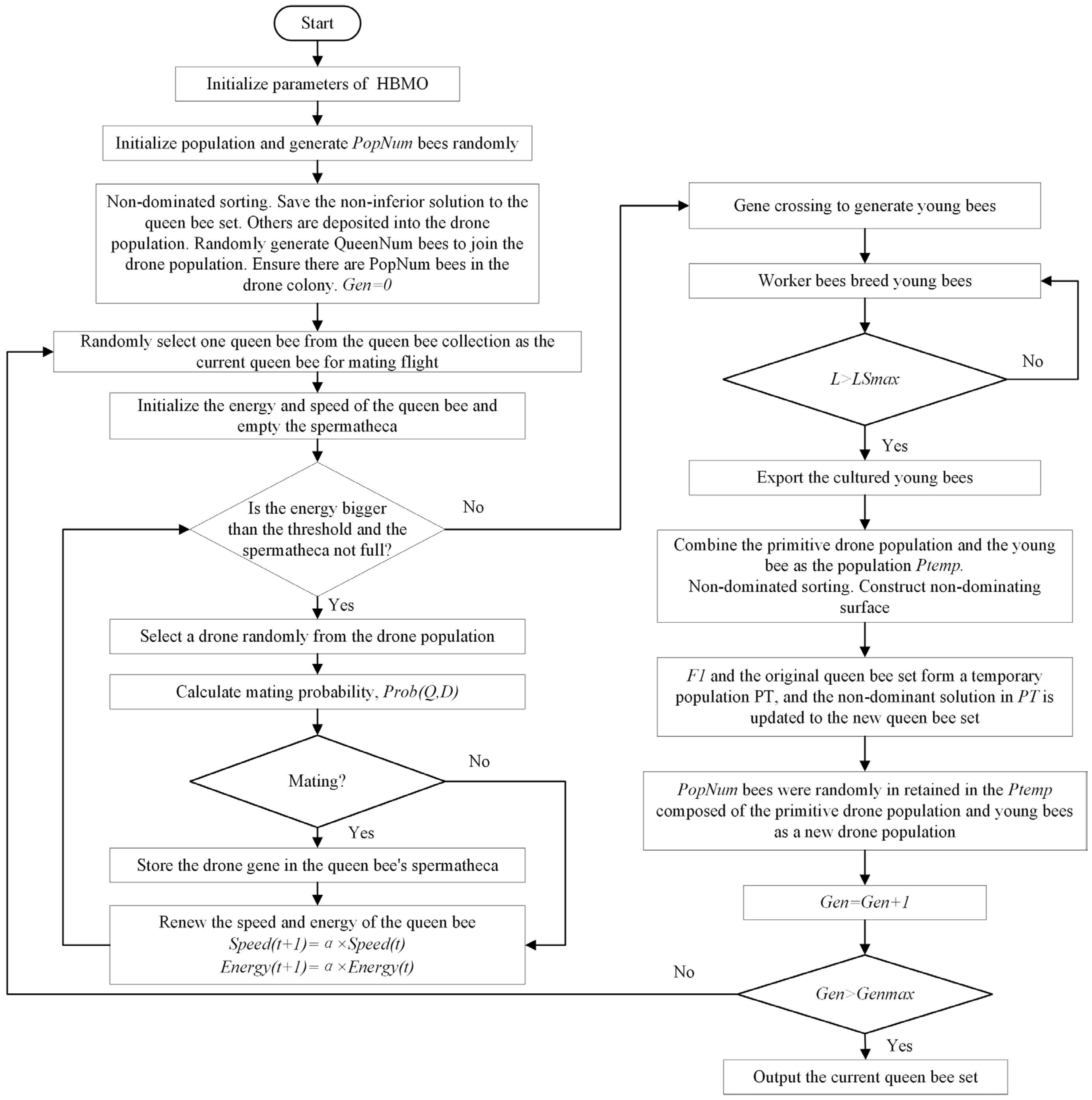
4. Proposed Improved HBMO Algorithm
4.1. Algorithm Design
4.2. Encoding and Decoding Design

| Parts | Machining Characteristics | Optional Machining Method | Operation Corresponding to Optional Method | Optional Machine Tool | Corresponding Processing Time of Machine Tool | Optional Cutter | Constraint Relation |
|---|---|---|---|---|---|---|---|
| Part 1 | F1; | Meth1 | 1op1 | M1, m2 | 13, 4 | T1, t2, t3 | Before F3 |
| Meth2 | 1op2 | M2, m3 | 4, 3 | T1, t2 | |||
| 1op3 | M1, m2 | 5, 4 | T3 | ||||
| F2; | Meth1 | 1op4 | M4, m7, m8 | 7, 6, 4 | T7, t8, t9 | ||
| Meth2 | 1op5 | M4, m5 | 3, 2 | T7 | |||
| 1op6 | M7, m8 | 3, 4 | T3, t4 | ||||
| About F3 | Meth1 | 1op7 | M7, m8 | 6, 4 | T4, t5, t6 | ||
| Part 2 | No. F4 | Meth1 | 2op1 | M2, m10 | 10, 5 | T3, t15, t16 | |
| Meth2 | 2op2 | M8, m9 | 4, 6 | T19, t20 | |||
| No. F5 | Meth1 | 2op3 | M3, m5 | 3, 7 | T2, t7, t13 | Before F6 | |
| Federal 6 | Meth1 | 2op4 | M1, m7 | 3, 9 | T5, t7 | ||
| 2op5 | M5, m10 | 6, 8 | T3, t8 | ||||
| Federal 7 | Meth1 | 2op6 | M3, m6 | 4, 8 | T2, t5 | Before F5 | |
| Part 3 | No. F8 | Meth1 | 3op1 | M6, m10 | 4, 5 | T11, t15, t16 | Before F9 |
| Meth2 | 3op2 | M8, m9 | 4, 6 | T19, t20 | |||
| No. F9 | Meth1 | 3op3 | M4, m9 | 3, 4 | T6, t7, t12 | ||
| No. F10 | Meth1 | 3op4 | M1, m3 | 3, 4 | T5, t6 | ||
| 3op5 | M2, m6 | 6, 4 | T4, t6 | ||||
| No. F11 | Meth1 | 3op6 | M2, m3 | 2, 4 | T6, t7, t12 |

4.3. Encoding Design
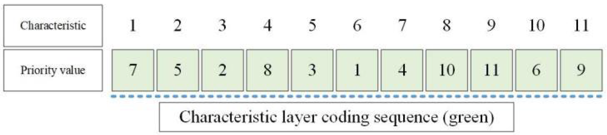
4.3.1. Encoding of Feature Layer
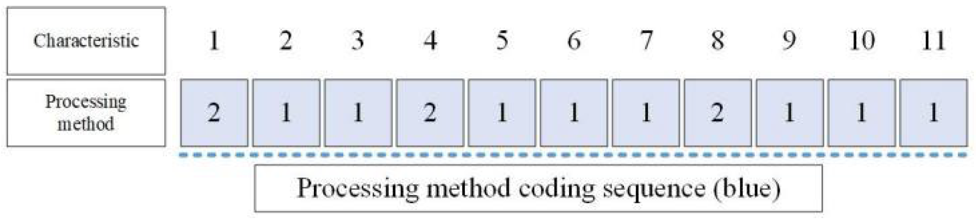
4.3.2. Encoding of Machining Method Layer
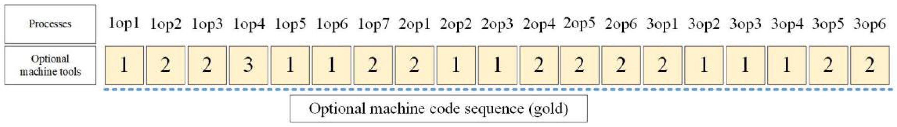
4.3.3. Machine Tool Layer Encoding
4.3.4. Encoding of Tool Layer
4.4. Decoding Operation
4.4.1. Decoding of Feature Layer
- Step 1:
- Find out the priority value of feature in the encoding sequence corresponding to column with all elements of the matrix being 0.
- Step 2:
- Compare the priority values of in the sequence, output the feature corresponding to the maximum value, and then set the priority value of the feature to zero in the encoding sequence.
- Step 3:
- Set row in matrix to zero.
- Step 4:
- Repeat the above steps until all features are output.
4.4.2. Decoding of Machining Method Layer
4.4.3. Decoding of Machine Tool Layer
4.4.4. Decoding of Tool Layer
4.4.5. Final Decoding
4.4.6. Chromosome Decoding Based on Greedy Algorithm
- Step 1:
- According to the above decoded process sequence and the corresponding machine tool and processing time, determine the processing machine tool set for each part and the processing process set for each machine tool.
- Step 2:
- Calculate the theoretical start time () of each process and the completion time of the process in the part before , .
- Step 3:
- Check the idle time of the process on the processing machine and obtain a series of idle time regions, . If , then make ; otherwise, check the next area. If all areas are not satisfied, then , in which is the completion time of the previous process on the same machine as .
- Step 4:
- From this, the start time () and completion time () of each operation can be obtained.
4.5. Young Bee Formation Stage
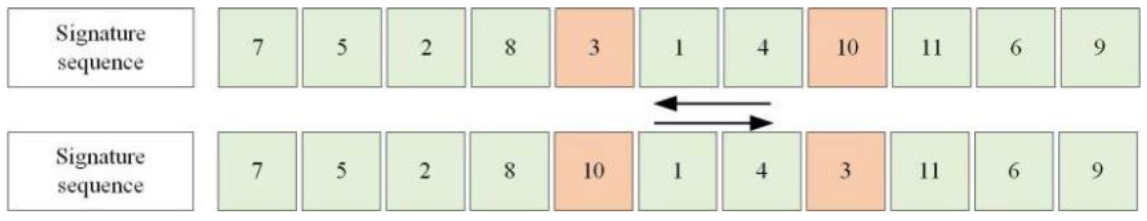
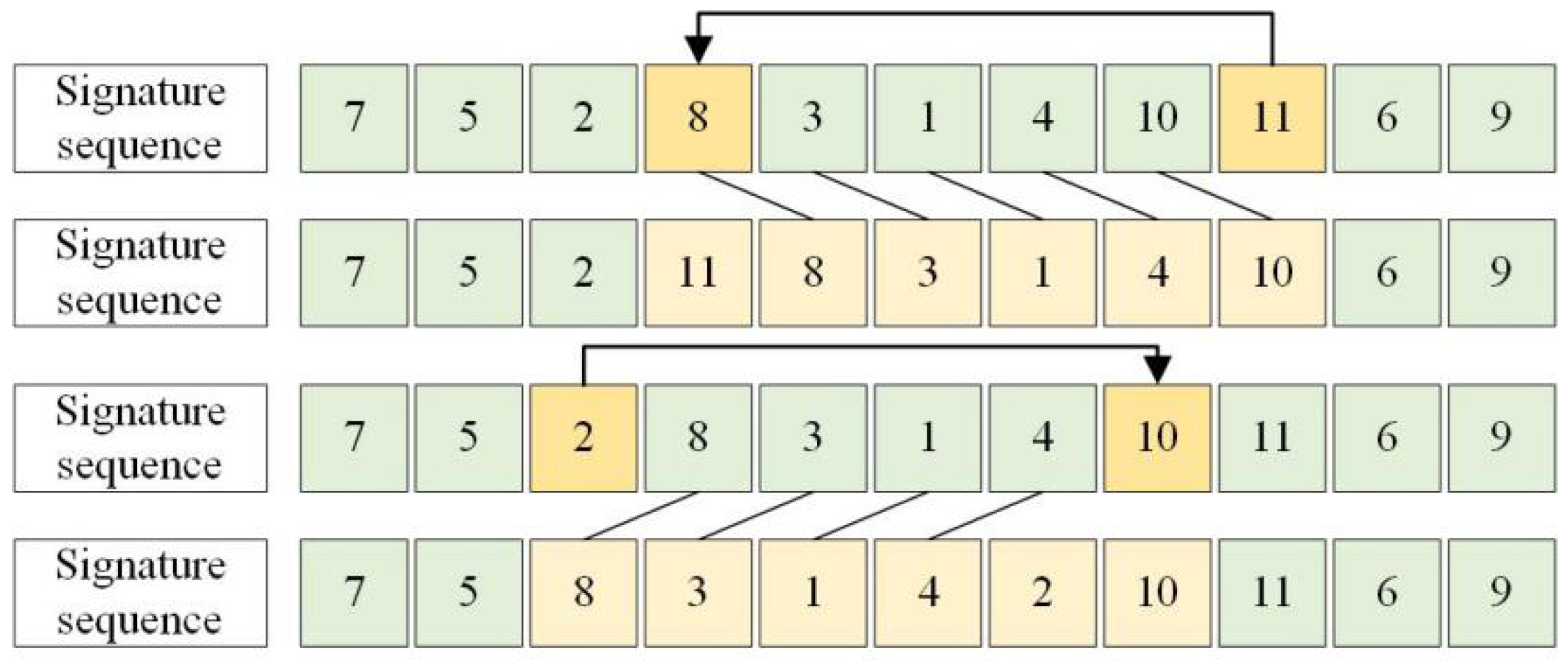
4.6. Crossover Operation of Feature Layer
4.7. Crossing of Process Layers
4.8. Cultivation Stage of Worker Bees
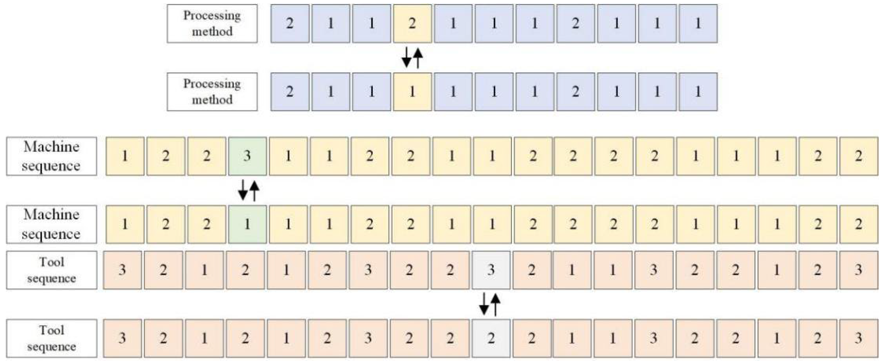
- (1)
- Exchange operation, : randomly select two different positions on the feature encoding sequence in young bees, and exchange the values at these two positions, as shown in Figure 9.
- (2)
- Insertion operation, : Randomly select a position on the feature encoding sequence in young bees, and insert the value at this position into any position on the sequence, and postpone the value of the gene site after insertion. The operation process is listed in Figure 10.
- (3)
- Mutation operation, : A gene locus in the processing method layer is randomly selected, and another processing method is selected according to its optional processing method. In the same way, one gene locus in the machine tool layer and tool layer is randomly selected, and another processing resource is selected according to its optional processing resources. The mutation operation process is given in Figure 11.
- Step 1:
- Set the maximum number of iterations for worker bees to breed young bees, so that , .
- Step 2:
- Randomly select a worker bee from an optional worker bee set, in which the young bee is cultivated to obtain a new young bee ; .
- Step 3:
- If the new young bee can dominate the young bee , use the young bee instead of the young bee , otherwise keep the young bee .
- Step 4:
- If not, jump to Step 2. Otherwise, the breeding process is terminated and the current young bees are exported; .
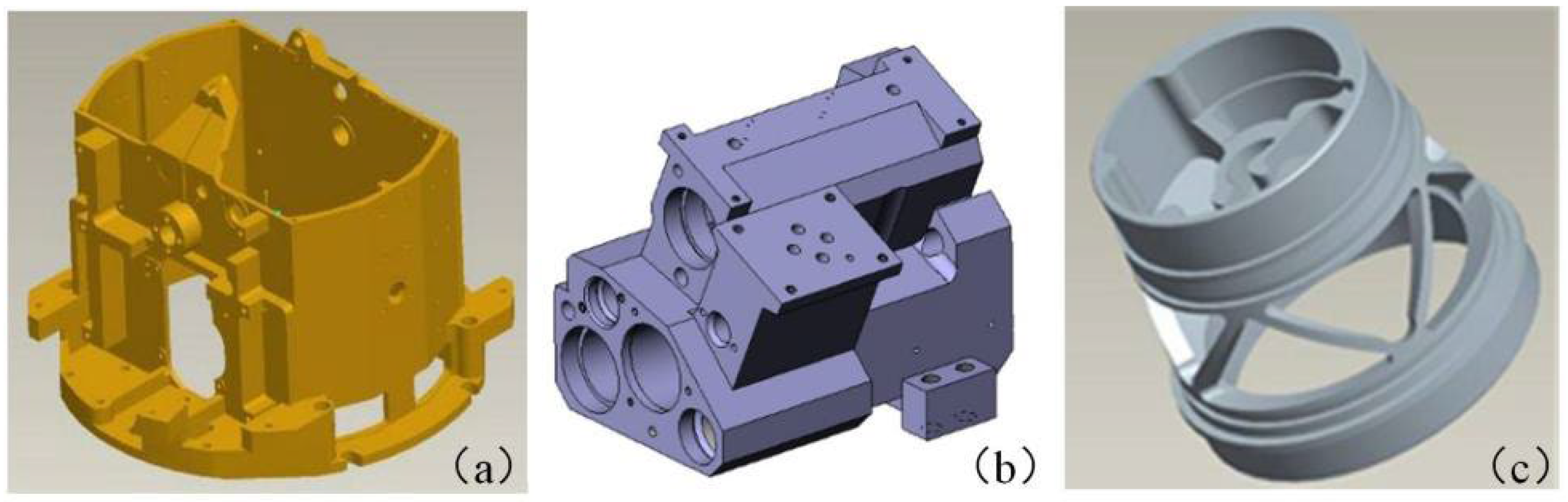
5. Case Analysis
5.1. Process Parameters
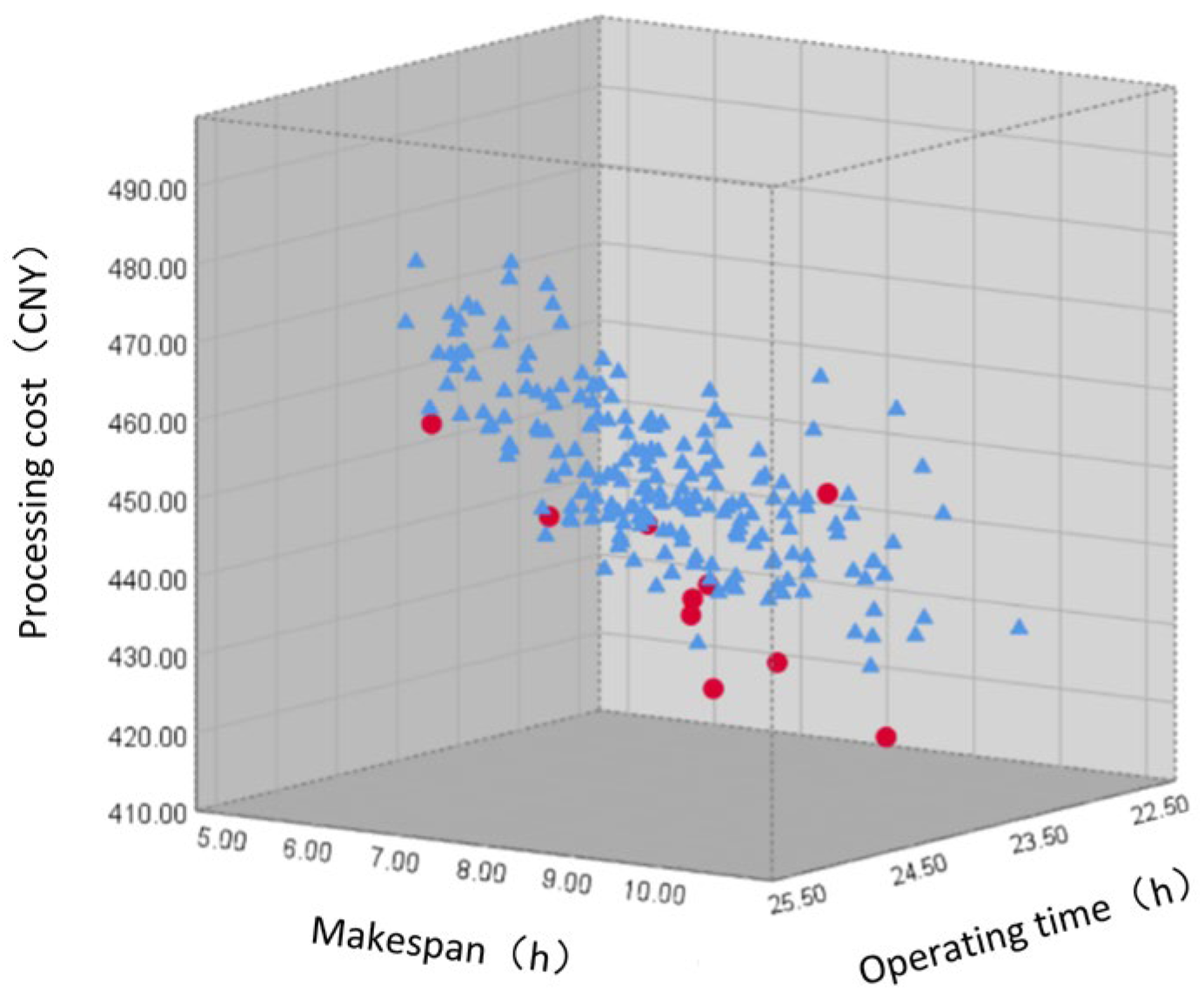
5.2. Efficiency Analysis of Improved HBMO Algorithm
- (1)
- The improved HBMO algorithm has set up a queen bee collection preservation mechanism based on the crowding degree in each generation of the iterative process, which can save the current non-inferior solution of the bee colony and participate in the generation of the next generation, ensure the transmission of excellent genes and promote the optimization of the algorithm.
- (2)
- Compared with the single mutation mechanism of the NSGA-II algorithm, the improved HBMO algorithm designs five kinds of breeding mechanisms for young bees in a local search, and breeds each young bee many times, adding better young bees to the population to replace the poor drones, ensuring that the population develops in a better direction after each iteration, which makes the algorithm have a better convergence effect.
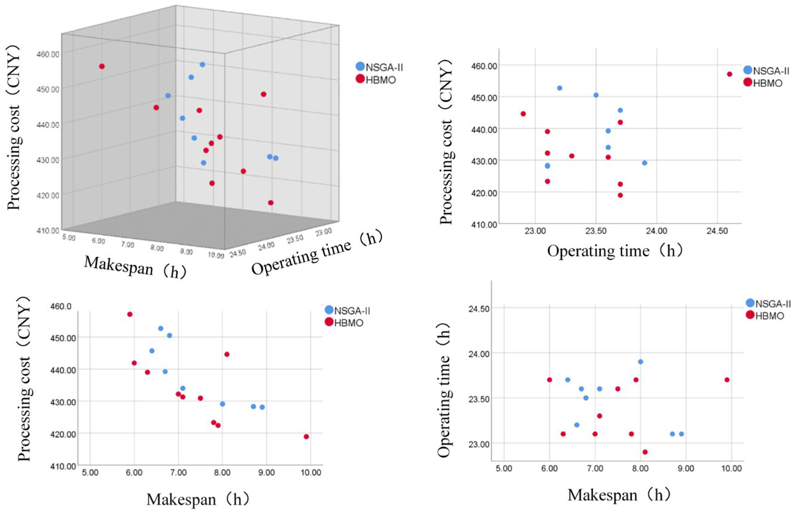
5.3. Analysis of Optimization Results
6. Conclusions
Author Contributions
Funding
Institutional Review Board Statement
Informed Consent Statement
Conflicts of Interest
References
- Tian, G.; Lu, W.; Zhang, X.; Zhan, M.; Dulebenets, M.A.; Aleksandrov, A.; Fathollahi-Fard, A.M.; Ivanov, M. A survey of multi-criteria decision-making techniques for green logistics and low-carbon transportation systems. Environ. Sci. Pollut. Res. 2023, 30, 1–23. [Google Scholar] [CrossRef] [PubMed]
- Zhang, F.; Mei, Y.; Nguyen, S.; Zhang, M. Evolving Scheduling Heuristics via Genetic Programming With Feature Selection in Dynamic Flexible Job-Shop Scheduling. IEEE Trans. Cybern. 2020, 51, 1797–1811. [Google Scholar] [CrossRef] [PubMed]
- Şahman, M.A. A discrete spotted hyena optimizer for solving distributed job shop scheduling problems. Appl. Soft Comput. 2021, 106, 107349. [Google Scholar] [CrossRef]
- Zhang, F.; Mei, Y.; Nguyen, S.; Zhang, M.; Tan, K.C. Surrogate-Assisted Evolutionary Multitask Genetic Programming for Dynamic Flexible Job Shop Scheduling. IEEE Trans. Evol. Comput. 2021, 25, 651–665. [Google Scholar] [CrossRef]
- Liu, Z.; Guo, S.; Wang, L. Integrated green scheduling optimization of flexible job shop and crane transportation considering comprehensive energy consumption. J. Clean. Prod. 2018, 211, 765–786. [Google Scholar] [CrossRef]
- Li, X.; Gao, L.; Shao, X.; Zhang, C.; Wang, C. Mathematical modeling and evolutionary algorithm-based approach for integrated process planning and scheduling. Comput. Oper. Res. 2010, 37, 656–667. [Google Scholar] [CrossRef]
- Lee, H.; Kim, S.-S. Integration of Process Planning and Scheduling Using Simulation Based Genetic Algorithms. Int. J. Adv. Manuf. Technol. 2001, 18, 586–590. [Google Scholar] [CrossRef]
- Li, X.; Gao, L.; Pan, Q.; Wan, L.; Chao, K.-M. An Effective Hybrid Genetic Algorithm and Variable Neighborhood Search for Integrated Process Planning and Scheduling in a Packaging Machine Workshop. IEEE Trans. Syst. Man Cybern. Syst. 2018, 49, 1933–1945. [Google Scholar] [CrossRef]
- Wen, X.; Lian, X.; Qian, Y.; Zhang, Y.; Wang, H.; Li, H. Dynamic scheduling method for integrated process planning and scheduling problem with machine fault. Robot. Comput. Manuf. 2022, 77, 102334. [Google Scholar] [CrossRef]
- Mohapatra, P.; Nayak, A.; Kumar, S.; Tiwari, M. Multi-objective process planning and scheduling using controlled elitist non-dominated sorting genetic algorithm. Int. J. Prod. Res. 2014, 53, 1712–1735. [Google Scholar] [CrossRef]
- Zhang, L.; Wong, T. An object-coding genetic algorithm for integrated process planning and scheduling. Eur. J. Oper. Res. 2015, 244, 434–444. [Google Scholar] [CrossRef]
- Xia, H.; Li, X.; Gao, L. A hybrid genetic algorithm with variable neighborhood search for dynamic integrated process planning and scheduling. Comput. Ind. Eng. 2016, 102, 99–112. [Google Scholar] [CrossRef]
- May, G.; Stahl, B.; Taisch, M.; Prabhu, V. Multi-objective genetic algorithm for energy-efficient job shop scheduling. Int. J. Prod. Res. 2015, 53, 7071–7089. [Google Scholar] [CrossRef]
- Salido, M.A.; Escamilla, J.; Barber, F.; Giret, A.; Tang, D.; Dai, M. Energy efficiency, robustness, and makespan optimality in job-shop scheduling problems. Artif. Intell. Eng. Des. Anal. Manuf. 2015, 30, 300–312. [Google Scholar] [CrossRef]
- Zhao, B.; Gao, J.; Chen, K.; Guo, K. Two-generation Pareto ant colony algorithm for multi-objective job shop scheduling problem with alternative process plans and unrelated parallel machines. J. Intell. Manuf. 2015, 29, 93–108. [Google Scholar] [CrossRef]
- Rohaninejad, M.; Kheirkhah, A.; Fattahi, P.; Vahedi-Nouri, B. A hybrid multi-objective genetic algorithm based on the ELECTRE method for a capacitated flexible job shop scheduling problem. Int. J. Adv. Manuf. Technol. 2014, 77, 51–66. [Google Scholar] [CrossRef]
- Chaudhry, I.A.; Usman, M. Integrated process planning and scheduling using genetic algorithms. Teh. Vjesn. Tech. Gaz. 2017, 24, 1401–1409. [Google Scholar] [CrossRef]
- Jin, L.; Tang, Q.; Zhang, C.; Shao, X.; Tian, G. More MILP models for integrated process planning and scheduling. Int. J. Prod. Res. 2016, 54, 4387–4402. [Google Scholar] [CrossRef]
- Zhang, S.; Yu, Z.; Zhang, W.; Yu, D.; Xu, Y. An Extended Genetic Algorithm for Distributed Integration of Fuzzy Process Planning and Scheduling. Math. Probl. Eng. 2016, 2016, 1–13. [Google Scholar] [CrossRef]
- Zheng, X.-L.; Wang, L. A knowledge-guided fruit fly optimization algorithm for dual resource constrained flexible job-shop scheduling problem. Int. J. Prod. Res. 2015, 54, 5554–5566. [Google Scholar] [CrossRef]
- Jiang, X.; Tian, Z.; Liu, W.; Suo, Y.; Chen, K.; Xu, X.; Li, Z. Energy-efficient scheduling of flexible job shops with complex processes: A case study for the aerospace industry complex components in China. J. Ind. Inf. Integr. 2021, 27, 100293. [Google Scholar] [CrossRef]
- Wang, W.; Tian, G.; Zhang, H.; Xu, K.; Miao, Z. Modeling and scheduling for remanufacturing systems with disassembly, reprocessing, and reassembly considering total energy consumption. Environ. Sci. Pollut. Res. 2021, 28, 1–17. [Google Scholar] [CrossRef] [PubMed]
- Yu, D.; Zhang, X.; Tian, G.; Jiang, Z.; Liu, Z.; Qiang, T.; Zhan, C. Disassembly Sequence Planning for Green Remanufacturing Using an Improved Whale Optimisation Algorithm. Processes 2022, 10, 1998. [Google Scholar] [CrossRef]
- Tian, G.; Fathollahi-Fard, A.M.; Ren, Y.; Li, Z.; Jiang, X. Multi-objective scheduling of priority-based rescue vehicles to extinguish forest fires using a multi-objective discrete gravitational search algorithm. Inf. Sci. 2022, 608, 578–596. [Google Scholar] [CrossRef]
- Wang, W.; Tian, G.; Yuan, G.; Pham, D.T. Energy-time tradeoffs for remanufacturing system scheduling using an invasive weed optimization algorithm. J. Intell. Manuf. 2021, 34, 1065–1083. [Google Scholar] [CrossRef]
- Tian, Z.; Jiang, X.; Liu, W.; Li, Z. Dynamic energy-efficient scheduling of multi-variety and small batch flexible job-shop: A case study for the aerospace industry. Comput. Ind. Eng. 2023, 178, 109111. [Google Scholar] [CrossRef]
- Yuan, G.; Yang, Y.; Tian, G.; Fathollahi-Fard, A.M. Capacitated multi-objective disassembly scheduling with fuzzy processing time via a fruit fly optimization algorithm. Environ. Sci. Pollut. Res. 2022, 28, 1–18. [Google Scholar] [CrossRef]
- Tian, G.; Zhang, C.; Fathollahi-Fard, A.M.; Li, Z.; Zhang, C.; Jiang, Z. An Enhanced Social Engineering Optimizer for Solving an Energy-Efficient Disassembly Line Balancing Problem Based on Bucket Brigades and Cloud Theory. IEEE Trans. Ind. Inform. 2022, 1–11. [Google Scholar] [CrossRef]
- Wang, W.; Tian, G.; Zhang, H.; Li, Z.; Zhang, L. A hybrid genetic algorithm with multiple decoding methods for energy-aware remanufacturing system scheduling problem. Robot. Comput. Manuf. 2023, 81, 102509. [Google Scholar] [CrossRef]
- Yang, Y.; Yuan, G.; Zhuang, Q.; Tian, G. Multi-objective low-carbon disassembly line balancing for agricultural machinery using MDFOA and fuzzy AHP. J. Clean. Prod. 2019, 233, 1465–1474. [Google Scholar] [CrossRef]
- Tian, G.; Liu, Y.; Tian, Q.; Chu, J. Evaluation model and algorithm of product disassembly process with stochastic feature. Clean Technol. Environ. Policy 2011, 14, 345–356. [Google Scholar] [CrossRef]
- Jiang, X.; Tian, Z.; Liu, W.; Tian, G.; Gao, Y.; Xing, F.; Suo, Y.; Song, B. An energy-efficient method of laser remanufacturing process. Sustain. Energy Technol. Assess. 2022, 52, 102201. [Google Scholar] [CrossRef]
- Feng, Y.; Zhang, Z.; Tian, G.; Fathollahi-Fard, A.M.; Hao, N.; Li, Z.; Wang, W.; Tan, J. A Novel Hybrid Fuzzy Grey TOPSIS Method: Supplier Evaluation of a Collaborative Manufacturing Enterprise. Appl. Sci. 2019, 9, 3770. [Google Scholar] [CrossRef]
- Fathian, M.; Amiri, B.; Maroosi, A. Application of honey-bee mating optimization algorithm on clustering. Appl. Math. Comput. 2007, 190, 1502–1513. [Google Scholar] [CrossRef]
- Niknam, T. An efficient multi-objective HBMO algorithm for distribution feeder reconfiguration. Expert Syst. Appl. 2011, 38, 2878–2887. [Google Scholar] [CrossRef]
- Marinakis, Y.; Marinaki, M. A hybrid Honey Bees Mating Optimization algorithm for the Probabilistic Traveling Salesman Problem. In Proceedings of the 2009 IEEE Congress on Evolutionary Computation, Trondheim, Norway, 18–21 May 2009; pp. 1762–1769. [Google Scholar] [CrossRef]


| References | Objective Functions | Scheduling Problems | Methodologies |
|---|---|---|---|
| Mohapatra et al. [9] | Makespan, idle time of machines, machining cost | IPPS | NSGA |
| Zhang et al. [10] | Makespan | IPPS | OCGA |
| Xia et al. [11] | Makespan | IPPS | GAVNS |
| Zhao et al. [14] | Makespan, machining cost | IPPS | ACO |
| Mohamad et al. [15] | Makespan, machining cost | IPPS | NSGA (ELECTRE) |
| Chaudhry [16] | / | IPPS | GA |
| This work | Makespan, machining time, machining cost | IPPS | HBMO |
| Symbol | Meaning | Symbol | Meaning |
|---|---|---|---|
| Number of parts to be processed | The first working procedure of the first machining method of the first characteristic unit of the part, | ||
| The first part in the parts to be processed, ; | The machining time on the machine tool of the first working procedure of the first machining method of the first feature unit of the part, | ||
| Number of machine tools available for machining | Cost per unit time of machine tool () | ||
| Number of tools available for machining | Cost per unit time of tool use () | ||
| The first machine tool, ; | The earliest completion time of the process on the machine tool ( ) | ||
| The first cutter, ; | Start time of working procedure on machine tool ( ) | ||
| The total number of feature units contained in the part ; | Decision variable; if selected as the machining method, take 1, otherwise take 0 ( ) | ||
| The first feature unit of a part, ; , | Decision variable; if selected as a machine tool, take 1, otherwise take 0 ( ) | ||
| Number of machining methods for the first feature unit of parts, | Decision variable; if the tool is selected, take 1, otherwise take 0 ( ) | ||
| Number of processes included in the first machining method of the first feature unit of the part, | The first processing method of the first characteristic unit of the part |
| Parts | Feature Number | Optional Machining Method | Process Corresponding to Machining Method | Optional Machine Tool | Machining Time Corresponding to Machine Tool (h) | Optional Cutter | Order Constraints between Features |
|---|---|---|---|---|---|---|---|
| Part 1 | F1 | Meth1 | 1op1 | 1/2/3 | 0.6/0.8/0.8 | T1/T2/T3 | Before all the features |
| 1op2 | 11/12 | 0.7/0.7 | T24/T25 | ||||
| Meth2 | 1op3 | 2/3 | 1.1/1.3 | T3/T4 | |||
| F2 | Meth1 | 1op4 | 11/12 | 0.8/0.8 | T24/T26 | Before F3/F4/F6 | |
| F3 | Meth1 | 1op5 | 1/2/3 | 0.5/0.6/0.6 | T2/T4 | ||
| F4 | Meth1 | 1op6 | 1/2/3 | 0.6/0.6/0.6 | T2/T4/T5 | ||
| Meth2 | 1op7 | 9/10 | 0.6/0.6 | T15/T16 /T17 | |||
| 1op8 | 9/10 | 0.7/0.7 | T18/T19 | ||||
| F5 | Meth1 | 1op9 | 1/2/3 | 0.9/8/0.9 | T1/T3/T4 | ||
| Meth2 | 1op10 | 4/5 | 0.4/0.6 | T9/T11/T12 /T13 | |||
| F6 | Meth1 | 1op11 | 1/2/3 | 0.7/0.5/0.9 | T1/T5 | ||
| Meth2 | 1op12 | 6/7/8 | 0.4/0.5/0.5 | No. 6/T7 /T12/T14 | |||
| Part 2 | F7 | Meth1 | 2op1 | 1/2/3 | 0.5/0.3/0.6 | T2/T3 /T4/T5 | Before all the features |
| 2op2 | 11/12 | 0.6/0.6 | T25/T26 | ||||
| F8 | Meth1 | 2op3 | 4/5/6 | 0.8/0.5/0.9 | No. 7/T8 /T10/T11/T12 | Before F9 | |
| 2op4 | 6/7/8 | 0.7/0.6/0.6 | No. 6/T8 /T10/T12 | ||||
| F9 | Meth1 | 2op5 | 4/5 | 0.9/8.8 | T9/T10/T14 | Before F10/F11/F12 | |
| 2op6 | 4/5/6 | 0.8/0.6/0.7 | T7/T11 /T12/T13 | ||||
| Meth2 | 2op7 | 5/6 | 0.7/0.7 | T9/T12 /T13/T14 | |||
| 2op8 | 5/6 | 0.7/0.7 | T9/T12 /T13/T14 | ||||
| F10 | Meth1 | 2op9 | 1/2 | 0.6/0.6 | No. T9/T10 /T11 | ||
| Meth2 | 2op10 | 1/2/3 | 0.6/0.6/0.5 | T4/T5 | |||
| 2op11 | 11/12 | 0.9/9 | T2/T3 /T4/T5 | ||||
| F11 | Meth1 | 2op12 | 9/10 | 0.6/0.6 | T24/T25 /T26 | ||
| Meth2 | 2op13 | 9/10 | 0.8/0.8 | T20/T21 | |||
| 2op14 | 9/10 | 0.6/0.6 | T18/T20 /T21 | ||||
| F12 | Meth1 | 2op15 | 1/2/3 | 0.8/0.6/0.7 | T1/T4/T5 | ||
| Part 3 | F13 | Meth1 | 3op1 | 4/5 | 0.8/0.6 | No. 7/T8 /T11/T14 | |
| Meth2 | 3op2 | 9/10 | 0.7/0.7 | T15/T16 /T17 | |||
| 3op3 | 9/10 | 0.9/9 | T22/T23 | ||||
| F14 | Meth1 | 3op4 | 6/7/8 | 0.6/0.7/0.7 | No. 7/T8 /T9/T10 | Before all the features | |
| 3op5 | 11/12 | 0.3/0.3 | T24/T25 | ||||
| Meth2 | 3op6 | 1/2/3 | 0.6/0.8/0.8 | T1/T2 /T4/T5 | |||
| F15 | Meth1 | 3op7 | 4/5 | 0.5/0.5 | T10/T11 /T12 | Before F17 | |
| Meth2 | 3op8 | 9/10 | 0.3/0.3 | T18/T19 /T20/T21 | |||
| F16 | Meth1 | 3op9 | 1/2/3 | 0.7/0.8/0.6 | T1/T2/T3 | ||
| F17 | Meth1 | 3op10 | 1/2/3 | 0.8/0.6/0.6 | T2/T3/T4 | ||
| Part 4 | F18 | Meth1 | 4op1 | 6/7/8 | 0.4/0.4/0.5 | T6/T7/T8 | Before all the features |
| 4op2 | 11/12 | 0.6/0.6 | T25/T26 | ||||
| F19 | Meth1 | 4op3 | 4/5/7/8 | 0.5/0.5/0.6/0.6 | No. 7/T8 /T9/T10/T13 | ||
| F20 | Meth1 | 4op4 | 4/5 | 0.6/0.5 | T10/T11/T14 | ||
| Meth2 | 4op5 | 9/10 | 0.3/0.3 | T15/T16 /T18/T19 | |||
| F21 | Meth1 | 4op6 | 9/10 | 0.6/0.7/0.7 | 6/T7/T9 /T11/T12 | ||
| Meth2 | 4op7 | 1/2/3 | 0.6/0.5 | T15/T16/T17 | |||
| 4op8 | 4/5/6 | 0.6/0.8 | T18/T20/T21 | ||||
| F22 | Meth1 | 4op9 | 1/2/3 | 0.4/0.4/0.4 | T2/T3/T4 | ||
| Meth2 | 4op10 | 4/5/6 | 0.5/0.5/0.6 | T7/T8/T11 /T12/T14 | |||
| 4op11 | 5/6/7 | 0.6/0.4/0.4 | No. 7/T8 /T12/T13 | ||||
| Part 5 | F23 | Meth1 | 5op1 | 1/2/3 | 0.5/0.6/0.6 | T1/T2 /T4/T5 | Before all the features |
| 5op2 | 1/2/3 | 0.5/0.5/0.5 | T2/T3/T5 | ||||
| Meth2 | 5op3 | 4/5 | 0.4/0.4 | T9/T10 /T11/T12 | |||
| F24 | Meth1 | 5op4 | 6/7/8 | 0.6/0.7/0.6 | T6/T7/T8 | ||
| F25 | Meth1 | 5op5 | 1/2/3 | 0.6/0.6/0.6 | T2/T3 | ||
| 5op6 | 4/5 | 0.3/0.4 | T10/T12 /T13/T14 | ||||
| F26 | Meth1 | 5op7 | 6/7/8 | 0.4/0.6/0.7 | No. 6/T8 /T9/T11 | ||
| F27 | Meth1 | 5op8 | 2/3 | 0.5/0.5 | T3/T4/T5 | Before F24 | |
| 5op9 | 6/7/8 | 0.6/0.4/0.5 | No. 7/T8 /T11/T14 | ||||
| Meth2 | 5op10 | 11/12 | 0.5/0.5 | T24/T25/T26 | |||
| F28 | Meth1 | 5op11 | 1/2/3 | 0.6/0.5/0.5 | T2/T4/T5 | ||
| Part 6 | F29 | Meth1 | 6op1 | 5/8 | 1.0/0.8 | T4/T5 /T7/T8 | Before F33 |
| F30 | Meth1 | 6op2 | 9/10 | 0.6/0.4 | T15/T16/T17 | Before F33 | |
| 6op3 | 4/6 | 0.3/0.5 | T7/T8 | ||||
| Meth2 | 6op4 | 9/10 | 0.6/0.4 | T15/T16/T17 | |||
| 6op5 | 6/7/8 | 0.5/0.5/0.4 | T6/T7/T8 | ||||
| F31 | Meth1 | 6op6 | 4/7/9/10 | 0.6/0.7/0.8/0.8 | T12/T13/T14 | Before all the features | |
| Meth2 | 6op7 | 4/5/7 | 0.6/0.5/0.7 | T12/T13/T14 | |||
| Meth3 | 6op8 | 1/2/3 | 0.6/0.6/0.8 | T12/T13/T14 | |||
| F32 | Meth1 | 6op9 | 4/5/6 | 0.8/0.9/0.7 | No. T9/T12 /T14 | Before F29 | |
| Meth2 | 6op10 | 9/10 | 0.4/0.4 | T18/T19 | |||
| 6op11 | 7/8 | 0.6/0.4 | T6/T7/T8 | ||||
| F33 | Meth1 | 6op12 | 1/2/3 | 0.8/0.6/0.6 | T1/T2/T3 /T4/T5 |
| Machine Tool Number | Name of Machine Tool | Type of Machine Tool | Machine Tool Cost per Unit Time (h/CNY) |
|---|---|---|---|
| China Net | Numerical control lathe | CK6163 | 12 |
| China Net | Numerical control lathe | CAK4085DI | 16 |
| China Net | Horizontal CNC lathe | CTX310V1 | 16 |
| China Net | Ordinary milling machine | 3 | 14 |
| Grand game | Three-axis NC vertical milling | KVC1050MA | 10 |
| China Net | Vertical CNC milling machine | DMU 35M | 16 |
| China Net | Drilling and milling machining center | TLV-500 | 12 |
| China Net | Numerical control vertical milling machine | VMP-32A | 12 |
| China Net | Boring and milling machining center | 1150 | 12 |
| China Net | Five-axis boring and milling machining center | UCP800 | 12 |
| Grand game | Vertical machining center | DMC63V | 16 |
| China Net | NC machining center | GX1000 Plus | 16 |
| Tool Number | Tool Cost per Unit Time (h/CNY) | Tool Number | Tool Cost per Unit Time (h/CNY) |
|---|---|---|---|
| T1 | 5 | T14 | 6 |
| T2 | 4 | T15 | 5 |
| T3 | 5 | T16 | 4 |
| T4 | 4 | T17 | 5 |
| T5 | 9 | T18 | 7 |
| T6 | 8 | T19 | 9 |
| T7 | 9 | T20 | 8 |
| T8 | 4 | T21 | 6 |
| T9 | 5 | T22 | 6 |
| T10 | 4 | T23 | 4 |
| T11 | 4 | T24 | 5 |
| T12 | 5 | T25 | 7 |
| T13 | 6 | T26 | 4 |
| Algorithm | F1 (h) | F2 (h) | F3 (CNY) | Algorithm | F1 (h) | F2 (h) | F3 (CNY) |
|---|---|---|---|---|---|---|---|
| HBMO | 7.9 | 23.7 | 422.4 | NSGA II | 8.7 | 23.1 | 428.3 |
| 6.0 | 23.7 | 441.9 | 8.0 | 23.9 | 429.1 | ||
| 8.1 | 22.9 | 444.6 | 6.7 | 23.6 | 439.2 | ||
| 7.1 | 23.3 | 431.3 | 7.1 | 23.6 | 434.0 | ||
| 6.3 | 23.1 | 439.0 | 6.4 | 23.7 | 445.7 | ||
| 7.5 | 23.6 | 430.9 | 8.9 | 23.1 | 428.1 | ||
| 9.9 | 23.7 | 418.9 | 6.6 | 23.2 | 452.7 | ||
| 7.0 | 23.1 | 432.2 | 6.8 | 23.5 | 450.5 | ||
| 5.9 | 24.6 | 457.1 | |||||
| 7.8 | 23.1 | 423.3 | |||||
| Optimum value | 5.9 | 22.9 | 418.9 | Optimum value | 6.4 | 23.1 | 428.1 |
| Average | 7.35 | 23.48 | 434.16 | Average | 7.4 | 23.46 | 438.45 |
| Serial Number | Maximum Completion Time (h) | Total Running Time of Machine Tool (h) | Cost of Machine Tools and Cutting Tools (CNY) | |||
|---|---|---|---|---|---|---|
| 1 | 7.9 | 23.7 | 422.4 | 0.004696 | 0.001815 | 0.278815 |
| 2 | 6.0 | 23.7 | 441.9 | 0.000114 | 0.010967 | 0.989697 |
| 3 | 8.1 | 22.9 | 444.6 | 0.005433 | 0.001439 | 0.209443 |
| 4 | 7.1 | 23.3 | 431.3 | 0.002103 | 0.004164 | 0.664419 |
| 5 | 6.3 | 23.1 | 439.0 | 0.000340 | 0.008575 | 0.961828 |
| 6 | 7.5 | 23.6 | 430.9 | 0.003352 | 0.002759 | 0.451465 |
| 7 | 9.9 | 23.7 | 418.9 | 0.011901 | 0.000189 | 0.015643 |
| 8 | 7.0 | 23.1 | 432.2 | 0.001817 | 0.004605 | 0.717034 |
| 9 | 5.9 | 24.6 | 457.1 | 0.000300 | 0.011865 | 0.975324 |
| 10 | 7.8 | 23.1 | 423.3 | 0.004317 | 0.002101 | 0.327352 |
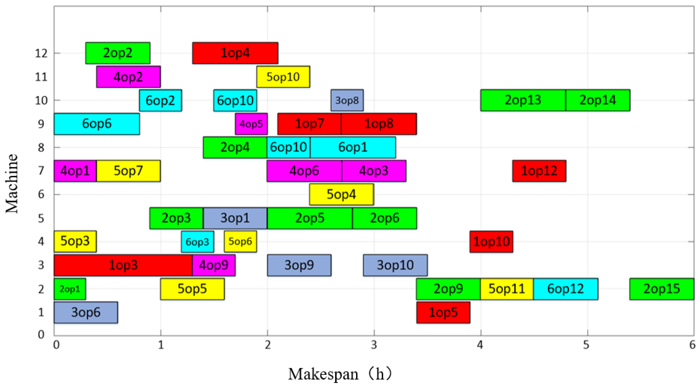
| Machine Tool | Processing Sequence |
|---|---|
| China Net | |
| China Net | |
| China Net | |
| China Net | |
| Grand game | |
| China Net | |
| China Net | |
| China Net | |
| China Net | |
| China Net | |
| Grand game | |
| China Net |
Disclaimer/Publisher’s Note: The statements, opinions and data contained in all publications are solely those of the individual author(s) and contributor(s) and not of MDPI and/or the editor(s). MDPI and/or the editor(s) disclaim responsibility for any injury to people or property resulting from any ideas, methods, instructions or products referred to in the content. |
© 2023 by the authors. Licensee MDPI, Basel, Switzerland. This article is an open access article distributed under the terms and conditions of the Creative Commons Attribution (CC BY) license (https://creativecommons.org/licenses/by/4.0/).
Share and Cite
Yang, G.; Tan, Q.; Tian, Z.; Jiang, X.; Chen, K.; Lu, Y.; Liu, W.; Yuan, P. Integrated Optimization of Process Planning and Scheduling for Aerospace Complex Component Based on Honey-Bee Mating Algorithm. Appl. Sci. 2023, 13, 5190. https://doi.org/10.3390/app13085190
Yang G, Tan Q, Tian Z, Jiang X, Chen K, Lu Y, Liu W, Yuan P. Integrated Optimization of Process Planning and Scheduling for Aerospace Complex Component Based on Honey-Bee Mating Algorithm. Applied Sciences. 2023; 13(8):5190. https://doi.org/10.3390/app13085190
Chicago/Turabian StyleYang, Guozhe, Qingze Tan, Zhiqiang Tian, Xingyu Jiang, Keqiang Chen, Yitao Lu, Weijun Liu, and Peisheng Yuan. 2023. "Integrated Optimization of Process Planning and Scheduling for Aerospace Complex Component Based on Honey-Bee Mating Algorithm" Applied Sciences 13, no. 8: 5190. https://doi.org/10.3390/app13085190