Numerical Performance of a Buoy-Type Wave Energy Converter with Regular Short Waves

Abstract

The numerical performance of a buoy-type wave energy converter (WEC) under regular wave conditions is described in this paper. The open-source computational fluid dynamics software OpenFOAM^® was used to couple a grid for the solid body motion of the WEC, with the grid designed for wave propagation, in order to calculate buoy movement parameters. The buoy has a horizontal, cylindrical structure, with a pivot point for semi-axis rotation. Five buoy-radiuses were analyzed, as this parameter considerably increases the efficiency of the WEC point absorber. To better understand the interaction of the WEC with the waves, the transmission and reflection coefficients were calculated, along with two non-linear parameters: skewness and asymmetry. The results indicate that, with this system, more power can be extracted from shorter waves, T = 4 s, compared to T = 8 s of the same wave height. This implies that a small buoy could be employed at sites with this prevailing wave regime, without a decrease in efficiency and with considerable cost reductions. Finally, this WEC increases the values of wave skewness, which is linked to onshore sediment transport; therefore, if appropriately designed, WEC arrays installed near the coast could also promote onshore sediment transport.

1. Introduction

Ocean waves constitute an important source of renewable energy, and its high energy potential along the coastlines of the world has been calculated to be 2.11 TW (to 95% confidence) [1]. Nevertheless, efficient energy extraction from ocean waves remains a considerable challenge. Many technologies have been developed and several are still under investigation. However, apart from the usual problems common to all renewables (e.g., fluctuation of the output power or non-competitive prices in energy production [2,3]), wave energy still faces several issues related to design optimization, the shapes and sizes of devices that attempt to harvest energy from an ever-changing and dynamic resource (intrinsic dynamics of the directional wave spectrum) [4,5]. This means that specific wave energy converter (WEC) technologies are best suited to a given set of wave conditions. Therefore, the estimation of wave energy availability must take this intrinsic condition into account, unless a very flexible technology adapted to all possible wave types is developed. Some of the more well-known devices are point absorbers, oscillating water columns (OWCs), attenuators (e.g., Pelamis), and overtopping/terminators (e.g., Wave Dragon); however, only a few of them have actually been used to generate energy from waves in practice.

An example of a device that was tested for a commercial phase is Pelamis Wave Power in Aguçadoura, Portugal. This was the first commercial wave energy farm in the world commissioned in 2008 with 2.25 MW of power generation supplied by three Pelamis devices; however, it only operated for a brief period due to technical difficulties with some bearings [6,7]. A second version of this device appeared in the UK in 2009, with 750 kW of power generation: the Pelamis P2 (from the Pelamis Wave company [7]) whose testing site was at the EMEC (European Marine Energy Centre) in the Orkney Islands, Scotland. Unfortunately, the company had financial difficulties in 2014 [8].

Another concept was Oyster 2, developed for Aquamarine Power, with a generation capacity of 800 kW; it was also installed and connected to the grid at the EMEC in June 2012. The test program ended in 2015 and the device is no longer in the water since the company ceased operations [9]. One other example is CETO devices, a submerged point absorber installed in 2010 in Fremantle, Australia, connected to the grid in 2015, with some of the excess energy production going into desalinating seawater. The commercial-scale CETO 6 unit commenced in 2017 with a 20 MW system, which could be expanded to 100 MW [10]. At present, these systems are being tested in Europe [11].

These cumulative experiences have been used to improve WEC technology and optimize the system’s performance. Notwithstanding, this kind of energy system is generally complex and expensive, with a relatively high cost of operation and maintenance [12]. Within the aspects that need to be considered in the performance of a WEC are the local environment and device characteristics, as well as the effect of other devices if we consider a wave energy farm [13]. It is also important to take into account the full cycle of the devices, from construction to the decommissioning and recycling of the parts, including its environmental impacts [14,15]. The complexity of wave energy technologies often goes hand in hand with their manufacturing and maintenance costs; therefore, a simple, tested, and optimized design could minimize costs and become commercially feasible [16].

One of the most important components that determine the energy harvesting efficiency of a point absorption device is the design of a buoy [17]. The buoy captures wave energy from the ocean and transfers this energy (by means of a power take-off mechanism) to a generator to be converted into electrical energy. The movement of the buoy is induced by the free surface waves and the maximum power absorption is attained when the point absorber is in resonance with the waves [18]. To find the optimal configuration, the shape and size of the buoy must be tested, as well as the degrees of freedom of the whole system and the flow field around it. In the absence of expensive wave basin facilities, and at the initial stages of development, the abovementioned goals can be partially attained with numerical simulations. In this regard, computational fluid dynamics (CFD) plays an important role in saving time and costs, as it is an excellent tool for the optimization and improvement of the design, which is created based on a performance analysis. The C++ libraries of the open source field operation and manipulation model, better known as OpenFOAM, are designed to solve several fluid mechanics problems [19]. Therefore, OpenFOAM is a CFD software suitable for analyzing a WEC design.

In recent years, OpenFOAM has been widely used to set up numerical wave tanks (NWTs) for the research and development of WECs as compared to other similar tools of its kind [20]. OpenFOAM can be used to model a particular device’s geometry with a good degree of accuracy; although, the runtime and high demand for computational resources are disadvantages [21]. During the simulation of WECs in an NWT, the mesh quality can decrease during the time of the simulation, since large distortions can appear due to the mesh design and vertical motion of the body (beyond the limits of the model stability [22]), or due to the presence of multiple floating objects [23]. There are many dynamic mesh motion methodologies to avoid mesh distortion; although, some can lead to numerical instability and, finally, to simulation crashes [20]. Examples are the ‘overset grid method’ (released in OpenFOAM since version v1706 and already validated [22]) and ‘mesh morphing method’. These two methods were recently assessed in WEC simulations [24], and although the overset grid method can accommodate large body displacements without mesh topological changes, it was found that it posed very high computational costs compared to the mesh morphing method [25]. The implementation of a CFD model could be a very complex process; hence, experience is required to create a correct numerical simulation. In addition, this may require a demanding mesh adjustment process when the motion of the device is coupled to the interaction with the fluid included in the simulation.

In this paper, OpenFOAM simulations are used to analyze the instantaneous power absorption of a cylindrical buoy that has a pivot point as the semi-axis of rotation, i.e., a point-pivoted absorber (PPA). The system is forced with regular waves and tested with a set of different buoy radiuses, where certain coefficients had to be modified to accommodate the correct mesh deformation. The subsequent sections are structured as follows. Section 2 addresses the governing equations applied to the fluid flow in the OpenFOAM model, their tools for the discretization of the domain, and the coefficients that describe the free surface deformation due to rigid body motion; a short description of the InterFoam solver, used for multiphase incompressible, isothermal, and immiscible fluids (water and air, in this study) is also included. Section 3 provides a brief explanation of the wave theory used in the simulations and the approaches for power calculations, along with an overview of the way in which the buoys, associated with WECs, absorb energy. Section 4 presents the numerical results of the model sensitivity analysis, the energy absorption by the different buoy diameters, and the effects that the WEC has on the modification of non-linear wave properties. In this section, discussions on mesh deformation, power absorption, and the potential effects on sediment transport due to the motion of the floating object are also included. Section 5 highlights the conclusions and recommendations.

2. Simulation Framework

2.1. Numerical Model

The CFD open source software OpenFOAM^® (v1912 version) was used to assess the efficiency of the device and perform the simulations. In the discretization of time and space domains for the Navier–Stokes equation, the solver applied the finite volume method using a grid over the fluid domain. For the NWT, the domain geometry was created with the blockMesh utility, which decomposes the domain in hexahedral blocks. For spatial discretization, the standard Gaussian integration by finite volume method was employed, which is based on the sum of the values of cell faces and interpolated from cell centers [26]. For the description of the fluid dynamics, the momentum equation in the volume of fluid (VOF) was defined for both air and water phases, assuming incompressible fluids and laminar flow existed. The Navier–Stokes equation for the conservation of momentum is given by:

$$\rho \frac{\partial \mathit{u}}{\partial t}+\rho \nabla \left(\mathit{u}\mathit{u}\right)+\nabla p=\nabla ·\left(\mu \left(\nabla \mathit{u}+{\left(\nabla \mathit{u}\right)}^T\right)\right)+\rho g$$

(1)

where, according to the Cartesian coordinates ($x,y,z$), $\mathit{u}$ describes the velocity vector field in the fluid, $\rho$ the density of the fluid, $p$ is the pressure, and $\mu$ the dynamic viscosity. Considering the conservation of the mass, the continuity equation for incompressible fluids is described by:

$$\nabla ·\mathit{u}=0$$

(2)

and the scalar equation for the water–air phase fraction can be written as:

$$\frac{\partial \alpha }{\partial t}+\nabla ·\mathit{u}\alpha +\nabla {\mathit{u}}_c\alpha \left(1-\alpha \right)=0$$

(3)

where ${\mathit{u}}_c$ is the compressive velocity. To delimit the free surface in the multiphase flow solver, the VOF method applies parameter $\alpha$, based on the volume fraction of each phase to differentiate the water and air interface, where $\alpha =1$ for water and $\alpha =0 \mathrm{for} \mathrm{the} \mathrm{air}$, and the phase volume fraction $0<\alpha <1$ represents the cell accommodating the water–air interface.

In the InterFoam solver, both the fluid and WEC motion are integrated. In each time step, the algorithm of the implicit motion solver updates the position, calculates the forces, and updates the acceleration, and then, moves the object at its new position. In the final step, the solver moves the mesh to accommodate the new changes, relative to the previous time step [27]. After the motion solver is evaluated, the fluid solver begins with the correction of the flow field by means of the VOF method using the multidimensional universal limiter for explicit solution (MULES), which considers a delimiter factor of the flow in the temporal solution. The following step in the procedure is to solve the momentum and pressure equation with the implementation of the pressure implicit method for pressure-linked equation (PIMPLE) algorithm. PISO (pressure implicit with splitting of operators) and SIMPLE (semi-implicit method for pressure-linked equation) algorithms were combined to achieve the PIMPLE algorithm. Within this PIMPLE algorithm, the following time step was begun until the maximum number of iterations was achieved, and this procedure was repeated until the end of the simulation. The complete method is detailed elsewhere [28].

2.2. Simulation Setup

The simulation set up focused on the buoy, which is the most important component of the point absorber that we tested. InterFoam was used as a dynamic mesh solver for isothermal immiscible fluids by means of the VOF phase fraction coupled to a 6 degrees of freedom (6-DoF) rigid-body motion solver (libraries sixDoFRigidBodyMotion [29]). The laminar flow version of the model was selected to avoid the use of a turbulence model in the flow simulation, since wave breaking is not necessary in the simulations. The properties of the two involved fluids are presented in

Table 1. Properties by phase.

	Units	Water	Air
Kinematic viscosity	${\mathrm{m}}^2·{\mathrm{s}}^{-1}$	$1.0\times {10}^{-6}$	$1.48\times {10}^{-5}$
Density	$\mathrm{kg}·{\mathrm{m}}^{-3}$	$1024$.0	1.0
Surface tension between the two phases	$\mathrm{N}·{\mathrm{m}}^{-1}$	$0.07$

.

The NWT was designed with the blockMesh utility, using the numerical domain geometry of 20 m in the $x$ direction, 5 m in the $y$ direction, and 6 m in the $z$ direction with a resolution of $\Delta x=\Delta y=\Delta z=1 \mathrm{m}$. Although the number of mesh elements was reduced at the ends of the NWT to reduce the computational time, a finer mesh was used for the area of interest surrounding the buoy to achieve more accurate results. The bounding box contained the pivot point of the buoy at coordinates (0, 0, 0). The NWT domain is schematized in Figure 1.

The buoy was a rigid, cylindrical body with a width $B=1 \mathrm{m}$, and a radius that was changed for the different tests (R = 0.1, 0.25, 0.5, 1.0, and 1.5 m). The buoy was connected to two arms of a constant diameter (0.03 m) and length $L_b$ that changed depending on the buoy’s radius (see

Table 2. Tested values for the buoy’s radius ^® and its arm length ($L_b$).

Buoy	$\mathit{R}\left(m\right)$	${\mathit{L}}_{\mathit{b}}\left(m\right)$	$\mathit{R}/{\mathit{L}}_{\mathit{b}}$
R1	0.10	1.5	0.067
R2	0.25	2.0	0.125
R3	0.50	3.0	0.167
R4	1.00	4.0	0.250
R5	1.50	6.0	0.250

). From R₁ to R₄, the ratio R/L_b increased proportionally to R, while the arms for R₄ and R₅ satisfied the same ratio R/L_b. The buoy’s density was ${\rho }_b=181.44 \mathrm{kg}· {\mathrm{m}}^{-3}$. The buoy was considered as a floating body with two constraints: the first one was a pivot point fixed at (0, 0, 0) to avoid back and forth movements, and, secondly, to only allow rotational movement only in the $x-z$ plane, i.e., the buoy had one degree of freedom in the rotation mode perpendicular to the direction of the incident wave. Other restraints were not considered, e.g., external forces, linear spring, linear damping, etc. The buoy was previously built in Stereolithography format (.STL file) in the open source software SALOME [30], and it was incorporated into the spatial domain using the snappyHexMesh tool. A detailed view of the buoy is presented in Figure 2 and the summary of the buoy’s properties is presented in Table 2.

For the spatial discretization of the boundary geometry, the inlet, outlet, sides, and top of the NWT were set as the patch type, where there was no geometric or topological information of the mesh; whilst the bottom (seabed) and the buoy were set as the wall type, geometries that interacted as solid objects. Through the inlet domain (at $x=-10$), the boundary condition imposed was Stokes’s wave theory, where the surface elevation $\eta$ occurs in the $z$ coordinate and the wave propagation occurs in the $x$ direction. Stokes waves propagate over a constant depth (h = 3 m). The activeAbsorption was set on the inlet and the shallowWaterAbsorption module was imposed on the outlet to absorb the incoming free surface water waves and prevent wave reflection. Another way to generate free surface waves in OpenFOAM is by means of the waves2foam toolbox; this library includes the relaxation zone technique to prevent the reflection of transmitted waves [31]. In this study, waves2foam toolbox was not used, and only those libraries included in OpenFOAM v1912 were employed. The tested wave properties included one amplitude only of $a=0.5 \mathrm{m}$ ($H=2a$) and wave periods for short and long waves (T = 4 s and T = 8 s, with wave steepness values of $H/\lambda =0.0527$ and $H/\lambda =0.0238,$ respectively). In this way, waves with lower and higher theoretical powers were tested (see subsequent section). During the initial conditions, when time step t = 0, the still water level (SWL) coincided with $z=0$ and the seabed had a constant water depth of h = 3.0 m along the XY plane. The time step was initially set as 0.01 s and, to conserve the numerical stability, an automatic adjustment of the time step was allowed based on the Courant number, rather than adopting a fixed time step.

In the alpha.water file, in the initial field for boundary conditions, zeroGradient was applied at the outlet, sides, buoy, and bottom, to avoid surface tension effects between the walls and water–air interface. Meanwhile, at the inlet and top, it was defined by waveAlpha and inletOutlet, respectively, with a value of 0. In the velocity file (U), the inlet and outlet boundaries were set up as waveVelocity type and the buoy patch was set as movingWallVelocity, whereas the top boundary was set as pressureInletOutletVelocity and the rest of the patches were set to fixedValue uniform at (0, 0, 0). In the case of pressure, all patches were set to fixedFluxPressure with a value of 0, except at the top, which was set as totalPressure (p0), which was evaluated by the model at every time step. Finally, only the buoy path was set as ‘calculated’, whereas the other patches were set as fixedValue uniform at (0, 0, 0) in the pointDisplacement file. This process is summarized in Figure 3.

Regarding the computational demand, all simulations were run on a 64-bit system with a memory of 31.3 GiB (processor intel^®Core™i7-6950X CPU @ 3.00 GHz × 20). To ensure consistency in the results of the numerical simulations, 100 wave periods were run for each individual test. The longest simulation lasted 3488 h using the computer resources available.

3. Calculations of Wave Power

3.1. Wave Power and Its Absorption by the Buoy

For the calculation of wave profiles and velocities, the 1st-order Stokes wave theory was employed. In unidirectional waves, the wave power per unit width of the wave front, or wave energy flux, can be estimated as [32]:

$$P_{wf}=C_g{E}_d$$

(4)

This equation is also known as the power density, since $E_d$ is the wave energy density ($\mathrm{J}/{\mathrm{m}}^2$) and $C_g$ is the group velocity ($\mathrm{m}/\mathrm{s}$).

According to the dispersion relationship, water waves can be classified by their relative depth as shallow water waves ($h/\lambda <1/20$), intermediate depth waves ($1/20<h/\lambda <1/2$), and deep-water waves ($h/\lambda >1/2$), where $\lambda$ is the wavelength and $h$ is the water depth. In the case of the numerical tests described in this manuscript, where $h=3$ m and wave periods are of 4 and 8 s, we considered intermediate depth waves, for which the power per wave front unit is defined as:

$$P_{wf}=\frac{\rho g^2}{16\omega }{H}^{2}D\left(\mathrm{kh}\right)$$

(5)

where H is the local wave height, $\omega$ is the angular frequency ($2\pi /T)$, $k$ is the wavenumber ($2\pi /\lambda$), $h$ is the water depth, and:

$$D\left(kh\right)=\left(1+\frac{2kh}{\sinh \left(2kh\right)}\right)\tanh \left(\mathrm{kh}\right)$$

(6)

The available power density can be related to the power absorbed by the WEC device through a parameter called the capture or absorption width [33], defined as the ratio of the power absorbed by the buoy ($P_{ab}$) to the available wave energy flux per unit crest length, and it is given by:

$$C_w=\frac{P_{ab}}{P_{wf}}$$

(7)

where $P_{ab}=\tau ·{\omega }_r$, where the torque $\tau$ and angular velocity ${\omega }_r$ are obtained by the analysis of the buoy’s movement. Since $P_{ab}$ is in W and $P_{wf}$ in W/m, $C_w$ has units in meters. Evans [34] established that, for axisymmetric bodies that are subjected to regular waves, the maximum theoretical capture width ratio is defined as:

$$C_{wMax}={ϵ}_{df}\frac{\lambda }{2\pi }$$

(8)

where $\lambda$ is the wavelength and the dimensionless value ${ϵ}_{df}$ is linked to the degrees of freedom. In WECs with a vertical axis of symmetry oscillating in heave mode $C_{wMax}=k^{-1}$ and for surge or pitch modes, as in our case, ${ϵ}_{df}=2$ [35]. In this sense, the ratio of the maximum extracted wave power to the available wave power flux from Equation (8) is equal to Equation (7), i.e., $C_{wMax}=P_{abMax}/P_{wf}$. This result implies that the buoy’s geometry is not related to the maximum $C_w$; rather, it is linked to the degrees of freedom. In conclusion, the shape of the floating object is independent of its maximum-capture width, which refers to the well-known antenna effect, where a small float can absorb waves over a width greater than its own dimension [36].

Regarding the energy conversion from the wave power available to the buoy, or the design of the device, different types of efficiency can be highlighted. One simple means to assess the capture efficiency, or hydrodynamic efficiency, is to divide the capture width (Equation (7)) by a characteristic length.

$$e_{cw}=\frac{P_{ab}}{P_{wf}B}=\frac{C_w}{B}$$

(9)

In this case, $B$ is such a length that represents the physical WEC length, or in our case, this would be the buoy width (see Figure 2). A more detailed description of the annual average capture width ratio of different WEC technologies can be consulted in [37].

On the other hand, the WEC efficiency is the ratio between the output power from the generator ($P_{out}$), and the power capture capability:

$$e_{WEC}=\frac{P_{out}}{P_{ab}}$$

(10)

Finally, the overall WEC efficiency, $e$, considering all the machinery of the device and its energy conversion, can be described as:

$$e=\frac{P_{out}}{P_{wf}B}=e_{cw}{e}_{WEC}$$

(11)

Note that the term $P_{ab}$ has disappeared from the right-hand side of the complete efficiency factor equation. This study focused on the effects of different buoy diameters on the performance of the power capture capability for a given set of wave characteristics, independent of the width of the buoy. Thus, Equations (7) and (8) are suitable for this purpose, whereas Equations (9) to (11) can be used when the results of this investigation are applied to physical experiments where $P_{out}$ can be calculated.

3.2. Bulk Parameters and Nonlinear Wave Properties

The extraction of renewable energy from ocean waves, via WEC devices, can alter coastal hydro- and morpho-dynamics. This may be due to the actual extraction process or to the WECs altering wave propagation (reflection, diffraction, and dissipation), which is especially important if the devices are placed close to the shore. It could be argued that the placing of WECs closer to the shore would be beneficial if the design of the WEC farm fulfils a double purpose: carbon-free energy generation and coastal protection [38].

A WEC device mounted on a buoy could act as a floating breakwater, dissipating wave energy and mitigating erosional effects on the coast. Two parameters are important in this case: the immersion ratio (the water depth above the device, divided by the water depth) and the relative length (the length of the buoy, divided by the water depth, $w/h$, where $w=L_b+R)$: in a brakewave, the reflection coefficients increase with the relative length [39]. A knowledge of the reflection, dissipation, and transmission coefficients produced by a WEC can be key to the installation of single or multiple devices. These types of wave bulk parameters are useful not only for assessing the effects on the coast, but also on other WECs, as in the case of a WEC farm or array, or on other marine structures. The reflection coefficient ($K_r$) is calculated as the ratio of the reflected and incident wave heights ($H_r/H_i$). This is usually evaluated where the incoming waves are approaching the WEC at the seaward end. The transmission coefficient ($K_t$) is defined as the ratio between the transmitted and incident wave heights ($H_t/H_i$). This is usually evaluated on the protected side of the WEC: the shoreward side. Finally, a coefficient must be added to compensate for the energy being dissipated or absorbed by the wave–structure interaction ($K_d$). This is calculated using the ratio between the assumed loss in wave height, denoted by $H_d$, to the incident wave height, $H_d/H_i$. This energy loss is related to the aforementioned coefficients to achieve wave energy conservation [40]:

$$K_t^2+K_r^2+K_d^2=1$$

(12)

According to Equation (12), the balance between reflected, transmitted, and dissipated wave heights must fulfil the following equation:

$$H_t^2+H_r^2+H_d^2=H_i^2$$

(13)

Equation (13) quantifies the wave energy loss as the wave field interacts with the WEC. In these experiments, $H_i$ and $H_r$ were evaluated with the gauges at points $P_1\left(-9.95,0,0\right)$, $P_2\left(-8,0,0\right)$, and $P_3\left(-7,0,0\right)$, with probe spacing values of $x_{12}=1.95$ and $x_{13}=2.95$.

Finally, for $H_t$, the point evaluated was $P_4\left(+10,0,0\right)$. Incident and reflected wave heights were measured by the methodology proposed by Mansard and Funke [41]. This method is based on applying a least squares method to separate the incident and reflected spectra assuming Fourier components on the decomposition of the free surface. They suggest the use of three gauges placed in the flume at suitable positions relative to the wavelength. We used 21 gauges, placed one meter apart in the $x$ direction. To quantify the wave energy absorption from a single WEC with the applied methodology [42], part of the wave height can be related to energy dissipation. This, in turn, is related to the energy absorbed by the buoy. Therefore, the wave energy absorption/dissipation ($H_d^2$) can be calculated from Equation (13) as $H_d^2=H_i^2-\left(H_t^2+H_r^2\right)$.

In this paper, a CFD model was used to assess the effects of the WEC buoy in modifying the non-linear wave properties known to contribute to onshore sediment transport, such as velocity skewness and vertical asymmetry [11,43]. The velocity skewness is defined as [44]:

$$s_k=\frac{\langle {\tilde{u}}^3\rangle }{\langle {\tilde{u}}^2\rangle {}^{3/2}}=\frac{\langle {\tilde{u}}^3\rangle }{{\tilde{u}}_{rms}^3}$$

(14)

where $\tilde{u}$ is the near-bottom oscillatory velocity and ${\tilde{u}}_{rms}$ is the free stream root-mean-square (RMS) velocity. Acceleration skewness or vertical wave asymmetry ($A_s$) can be calculated as [44]:

$$A_s=\frac{\langle \mathcal{H}{\left(\tilde{u}\right)}^3\rangle }{\langle {\tilde{u}}^2\rangle {}^{3/2}}$$

(15)

where $\mathcal{H}\left(\tilde{u}\right)$ is the Hilbert transform of the oscillatory velocity. For the simulation, the wave gauges used to record the wave velocity were placed every meter from $x=-10$ to $x=10$, and with $y=0$ and $z=-2.75$.

4. Results and Discussion

4.1. Execution Time and Model Stability

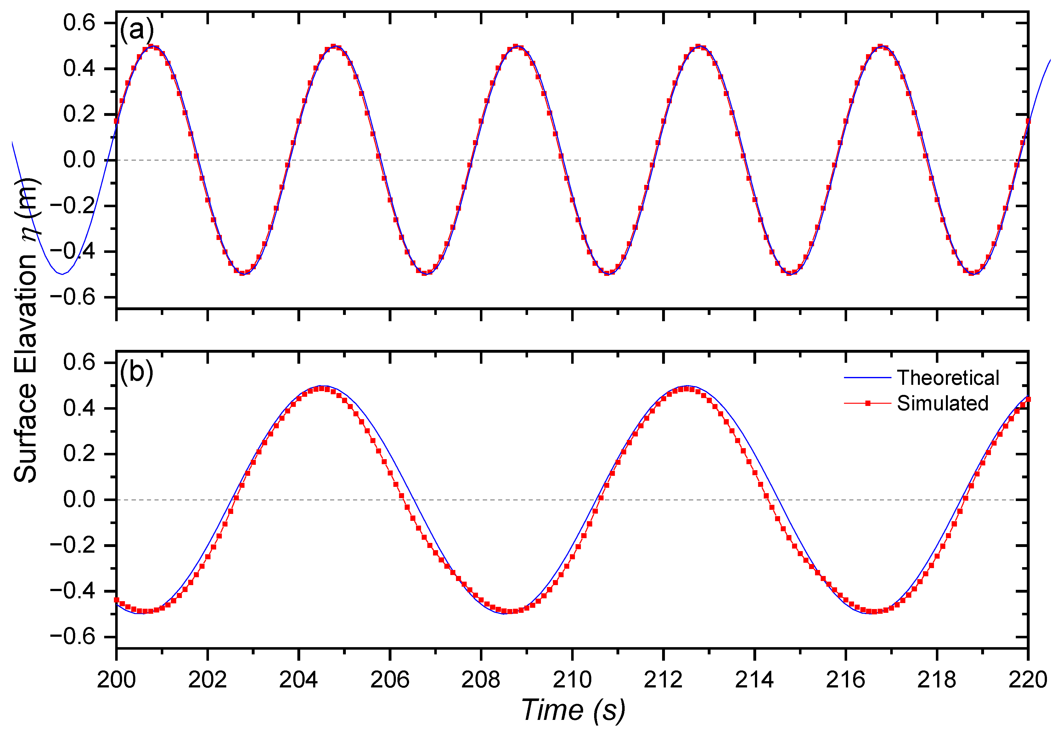
Figure 4 shows a comparison of the free surface data from the simulations and the theoretical results, calculated at the inlet boundary of the NWT. The free surface was accurately reproduced by OpenFOAM and the motion of the floating bodies under wave action was validated and corresponded well with the reported experimental data [45,46]. A similar case to the present simulation was recently presented by Qu et al. [47], who studied the hydrodynamic forces of semi-submerged horizontal, rectangular, and circular prisms. In their validation process, the free surface of theoretical and simulated waves was compared, with a relative variation of 1.08%.

It can be seen from Figure 4 that there is no significant difference between the theoretical and simulated free surfaces. Hence, the result from this simulation setup is considered to be in agreement with the quality of the mesh. The extra setup of the NWT to assess the set of subsequent cases was not necessary. As previously mentioned, the limitations of a simulated approach obliged us to treat the results of the current study with caution.

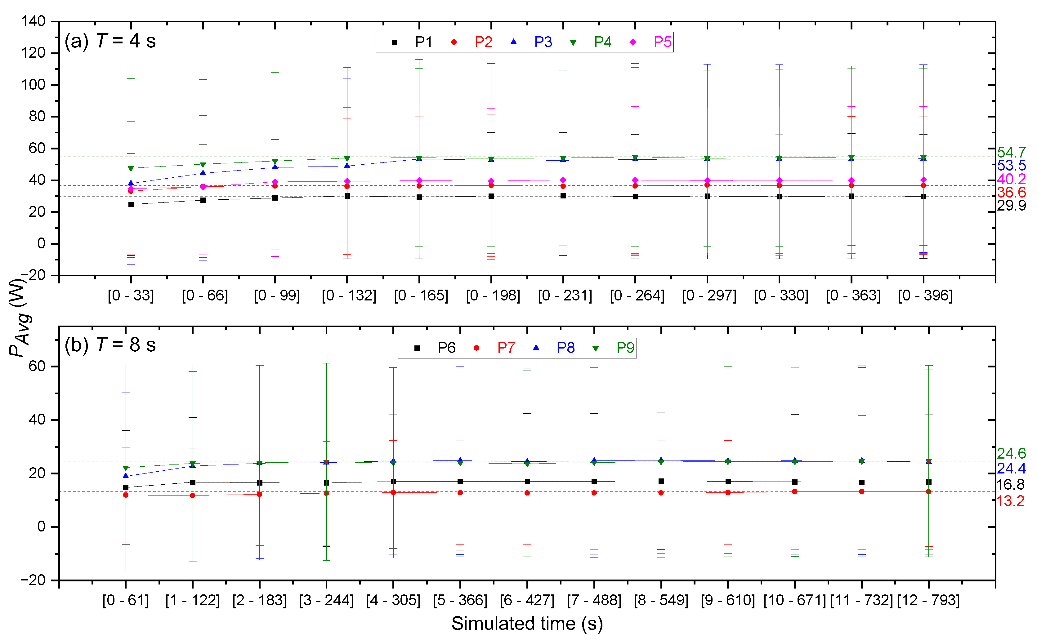
The results, in relation to the average power delivered, show that after a few wave periods, the averages and standard deviations of the model simulations do not change significantly, as shown in Figure 5 (the parameters for each simulation from P1 to P9 are described later in Section 4.2).

The execution time for the simulation of one hundred waves is presented in Figure 5 and the computation time is resumed in

Table 3. Computation time using the mesh morphing method.

$\mathrm{Buoy}$	T = 4 s	T = 8 s
	Computation Time (Hours)
$R_1$	127.23	260.23
$R_2$	226.01	491.94
$R_3$	615.93	1246.81
$R_4$	1196.84	2390.67
$R_5$	2027.45	3488.00

. It can be seen that the computation time increases as the buoy’s size increases. It is worth mentioning that the computation time using the overset grid method is double the runtime of that using the mesh morphing method, making the former considerably more demanding, computationally [24].

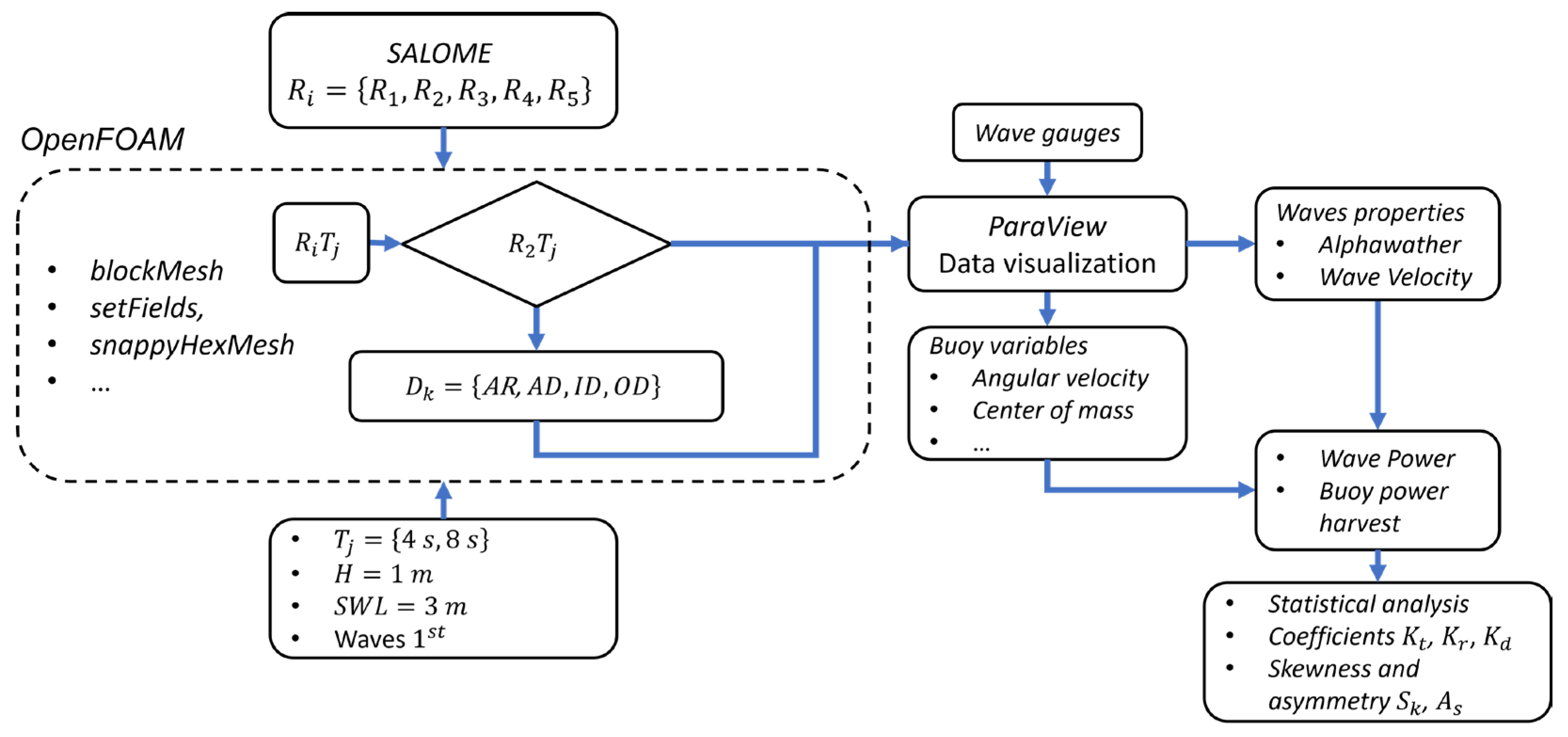
4.2. Sensitivity Tests

This section describes the sensitivity analysis performed to identify the body motion parameters where the results were more sensitive and prone to changes. These parameters were Acceleration Relaxation (AR), which acts to reduce the acceleration directly; Acceleration Damping (AD), used to eliminate the divergence generated from sudden acceleration events and proportional to the magnitude of the acceleration; Inner Distance (ID), the extension of the region of motion of the fluid around the solid body; and, finally, Outer Distance (OD), which refers to the extent of the mesh transformation region around the body. The inner and outer distances are equivalent to diffusivity; however, as a function of distance. In reviewing the literature, not much information was found on these body motion parameters and few authors mention the topic, e.g., Windt et al. [22,25] investigated mesh morphing and overset grid methods, comparing their results with the data from an experimental tank of the WaveStar device, inferring that the use of the overset grid method is computationally more expensive and a thorough model setup is required; hence, inner and outer distances could be parameterized by the buoy’s radii or length. The adopted values here are within the ranges previously considered. The grid points in the range ID < D < OD were deformed while the object was moving and, often, the ID values were in the order of the boundary layer thickness, and OD was limited by the nearest domain boundary [48,49].

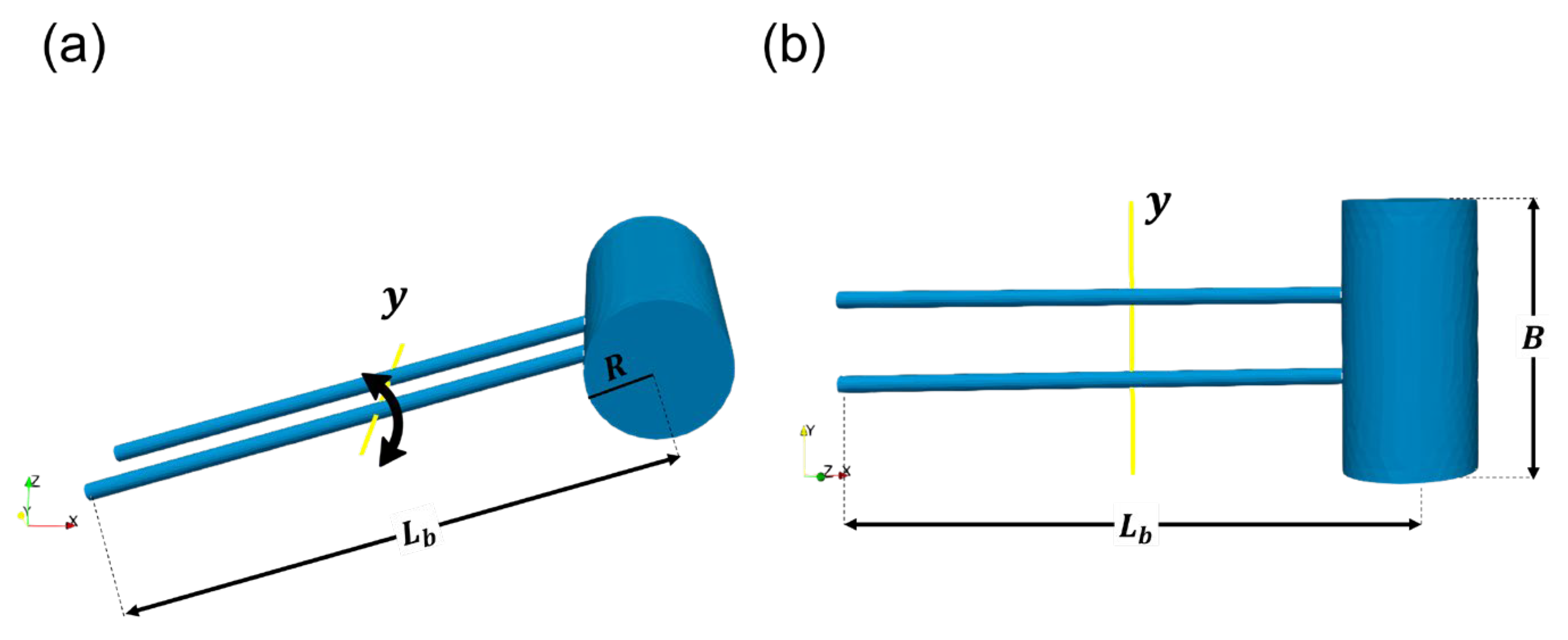
The analysis was performed considering the variation in the coefficients at a constant radius R = 0.25 m, and the values are shown in

Table 4. Coefficients of the simulation cases for the sensitivity tests for H = 1.0 m, T = 4 s, and 8 s, conducted for a buoy with R = 0.25 m.

Case	T (s)	AR	AD	ID	OD
P1	4	0.7	1.0	0.001	1.5
P2		0.7	1.0	0.001	2.0
P3		0.5	0.5	0.001	1.5
P4		0.5	0.5	0.00001	1.5
P5		0.7	0.75	0.001	1.5
P6	8	0.7	0.75	0.001	1.5
P7		0.7	1.0	0.001	1.5
P8		0.5	0.5	0.001	1.5
P9		0.5	0.5	0.00001	1.5

. The simulations were labeled as P1 to P9, performed for periods of 4 and 8 s. For each test, a total of 100 wave periods was simulated without crashing. The nine cases presented in Table 4 were divided into five groups, testing a combination of different parameters.

Table 5. Sensitivity tests to evaluate the effects of the parameters AD, ID, and OD in the simulations.

Test Number	Sensitivity Test	Cases Compared
1	OD-4T	P1, P2
2	ID-4T	P3, P4
3	AD-4T	P1, P5
4	AD-8T	P6, P7
5	ID-8T	P8, P9

shows the P1–P9 tests that were labeled after the parameter examined in addition to the wave period. For example, in test OD-4T, cases P1 and P2 were compared, where only the Outer Distance parameter was modified and the rest remained unchanged; test ID-4T analyzed the differences between P3 and P4, where only the Inner Distance parameter was modified, and so forth. The analysis of the AR parameter was omitted because no considerable effect was noted for the adopted values, which represent the rate of the decrease in acceleration.

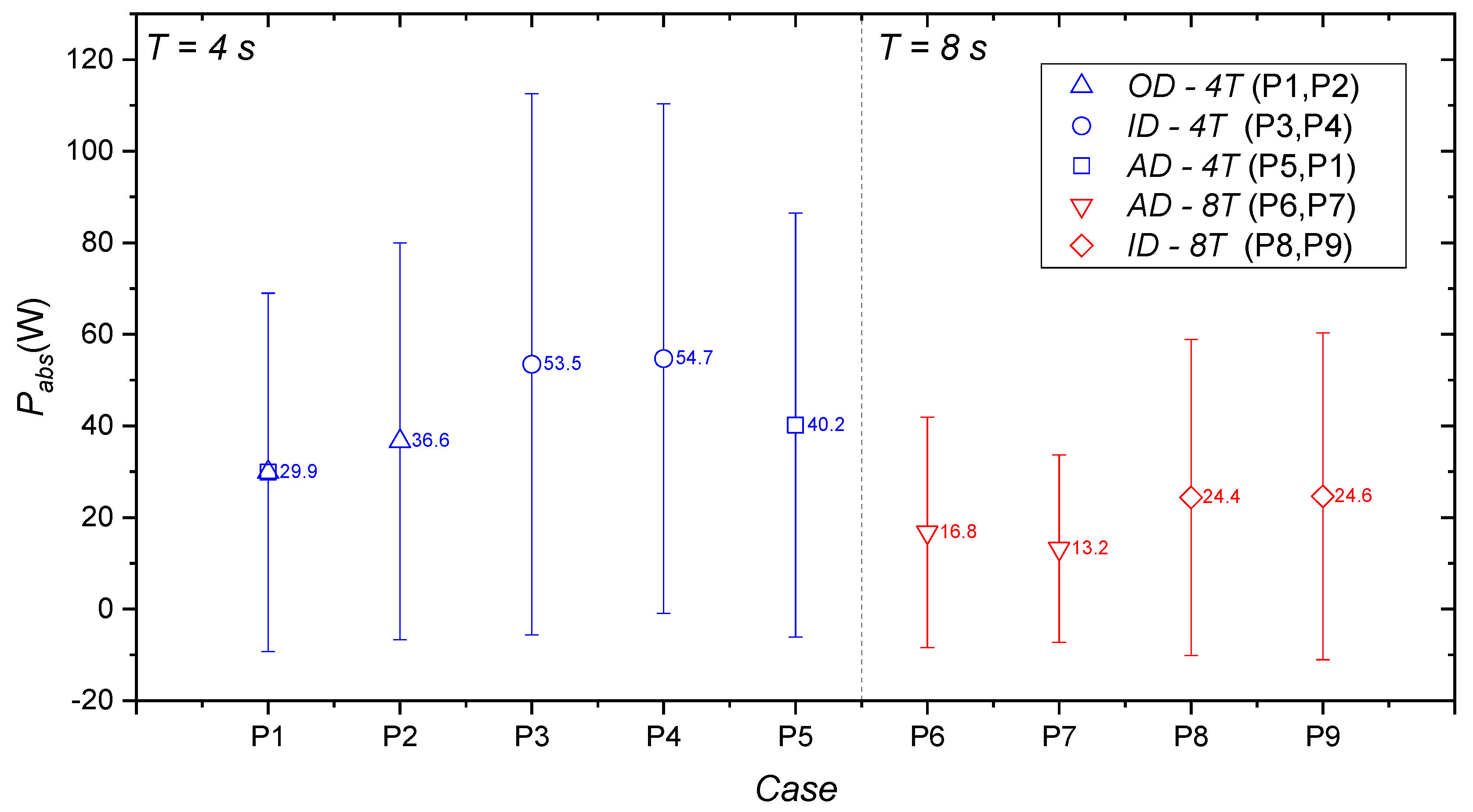
These tests were initially assessed by calculating the instantaneous power by multiplying the instantaneous values of the torque ($\tau$) and angular velocity (${\omega }_r$): the output power was calculated as the average of the instantaneous power over the time of the simulation. The results for the nine cases are presented in Figure 6; there were no significant differences in the execution times since all were performed with a 0.25 m buoy. As shown in Figure 6, an increase in the OD coefficient induces an increase in the average power and its standard deviation. Changes in the ID did not show significant changes in the mean power (at least in the evaluated values). On the other hand, changes in the AD had considerable effects on the mean power and its standard deviation, at least for the shorter-period waves (4T) where the mean values were 34% higher. If a default value of AD = 1 was set, it produced the minimum value of the output power. In order to avoid a power overestimation, this would be the preferred setting.

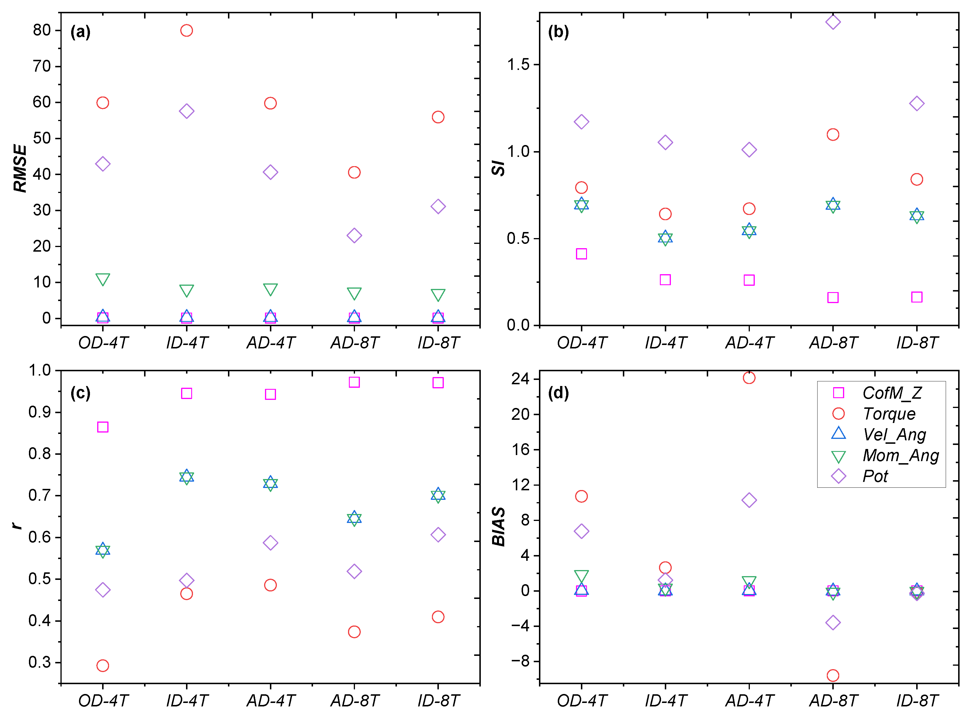
To complement the results presented in Figure 6, a further analysis was conducted by using the time series of other available variables, such as the center of mass of the buoy (CofM_Z), its angular momentum (Mom_Ang), its angular velocity (Vel_Ang), and the torque. Since the output power depends on both the angular velocity and torque, values of power (Pot) were also included in the analysis. The statistical parameters, calculated for each of the time-series pairs (test numbers in Table 5), included (i) the root mean square error (RMSE), to denote the magnitude of the error in the same units of the variable (small values of this parameter indicate a greater similarity between the cases in Table 5); (ii) the scatter index (SI), which indicates the error percentage, calculated by dividing the RMSE by the average of the model; (iii) the Pearson’s correlation coefficient, denoted as r and ranging from −1 to +1, which defines the linear relationship as negative or positive, or the absence of a correlation (r ~ 0); and, finally, (iv) BIAS, a measure of the tendency for underestimation (overestimation) when negative (positive) values are found.

Figure 7 shows the results obtained from the statistical analysis. The center of mass (CofM_Z) seems to be the best-performing variable, with low RMSE and SI values and a fairly high linear correlation, and showing very little effect of changing OD, ID, or AD. On the other hand, the torque seemed to be the variable with the highest RMSE values of all the tests performed, with the changes in ID being those that affected the RMSE the most. Torque was also the variable that showed the lowest linear correlation r, especially for changes in ID and AD. Changes in the latter coefficient also had the highest values of positive bias (see Figure 7d). The statistics for the angular velocity had fairly low RMSE and SI values, respectively, and its BIAS was fairly close to zero. This is a great advantage since the calculations of power rely on both torque and angular velocity.

As no physical experiments were available for validation, the criteria for choosing the combination of parameters to use were those providing lower values of power BIAS and of power RMSE, and those avoiding high overestimations for the torque. Those characteristics were found in the tests where the AD was fixed to the default value of 1 (P1 and P7). It was noted on several tests, performed but not reported here, that drastic changes in these parameters could induce the instability of the model through excessive mesh distortion. The results using the OpenFOAM model prove to be in agreement with the experimental data when the correct parameters are applied, with its respective assumptions and limitations [50].

4.3. WEC Power Absorption

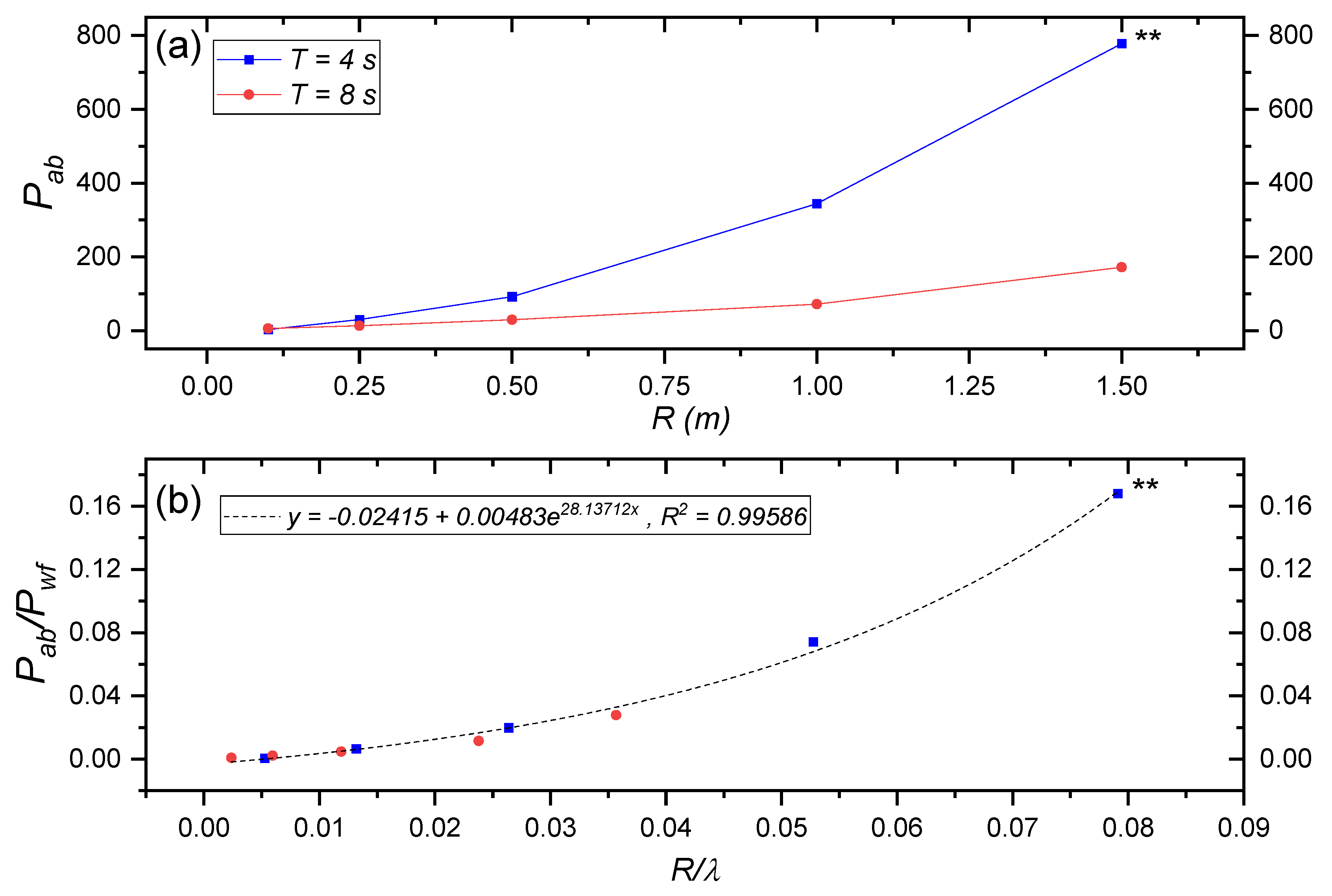
The values of the parameters from the sensitivity tests were then fixed in order to evaluate the changes in the buoy’s radius, systematically. These values were presented in the P1 and P7 cases in Table 1 (AR = 0.7, AD = 1, ID = 0.001, and OD = 1.5). As we expected, the average power output increased with the buoy’s radius, as can be seen in Figure 8a; perhaps, surprisingly, shorter-period waves (T = 4 s) delivered considerably more average power with this buoy system than waves of longer periods (T = 8 s). It is also apparent from Figure 8a that 4 s waves induce an exponential power increase with an increasing buoy radius, while the power values for the buoy with longer-period waves (T = 8 s) suggested a much slower increase rate. On the other hand, Figure 8b seems to suggest that the capture efficiency ($y$-axis) of a buoy whose size is a given fraction of the wavelength ($x$-axis) would be very similar for both T = 4 s and T = 8 s waves. Here, is important to note that the 1.5 m case for T = 4 s could not be run with a value of OD = 1.5 due to instabilities caused by the buoy’s movement and increased size of the buoy on the mesh. Therefore, a value of OD = 2 had to be adopted, which could imply a 1.2% error for the mean values of the average power absorbed (see values of SI presented in Figure 7b).

The results presented in Figure 8 have significant implications for the assessment of wave energy availability, and also for the manufacturing of WECs of the type presented in this paper. For example, if we only rely on the results of the wave energy flux (Equation (4)) of a given site, to assess the wave energy availability, we would expect that a site with longer-period waves (i.e., T = 8 s) would generate more energy than a site with shorter-period waves (i.e., T = 4 s) per unit wave height. Nevertheless, in these experiments, using a R = 1 m buoy, T = 4 s waves captured considerably more energy, a factor of 4.82, than T = 8 s waves (Figure 8a). This factor seems to increase in an exponential fashion with an increased radius. This implies that, in order to achieve the same capture efficiency, T = 4 s waves need much smaller buoy diameters than T = 8 s waves, making the devices cheaper to manufacture. For example, to achieve a capture efficiency of 0.16 at a 3 m depth, a T = 8 s wave would need a buoy with a radius of 3.36 m ($R/\lambda$ = 0.08), whereas of T = 4 s wave needs a buoy half the size (1.5 m). Therefore, with the technology we tested in this paper, regions where shorter-period waves dominated (enclosed seas) generated more energy and with a cheaper device than regions dominated by longer-period waves. These results are in agreement with the results observed elsewhere [51]. Consequently, with the results presented in this work, the availability of ocean wave energy has a high dependence on the technology used to harvest it, and should be considered in techno-economic assessments.

To assess the amount of energy absorbed by the system, the results obtained from the calculation of the bulk energy balance (Equation (12)) were analyzed, where the values of $K_d^2$ could be interpreted as the amount of energy that was absorbed by the WEC or dissipated through turbulent processes.

Table 6. Coefficients of energy transmitted ($K_t^2$), reflected ($K_r^2$), and absorbed/dissipated ($K_d^2$) for different buoy sizes and during the two wave periods.

Buoy	T = 4 s			T = 8 s
	${\mathit{K}}_{\mathit{t}}^2$	${\mathit{K}}_{\mathit{r}}^2$	${\mathit{K}}_{\mathit{d}}^2$	${\mathit{K}}_{\mathit{t}}^2$	${\mathit{K}}_{\mathit{r}}^2$	${\mathit{K}}_{\mathit{d}}^2$
$R_1$	0.298	0.005	0.698	0.477	0.006	0.517
$R_2$	0.300	0.004	0.695	0.489	0.006	0.506
$R_3$	0.298	0.005	0.698	0.484	0.005	0.511
$R_4$	0.290	0.006	0.704	0.480	0.005	0.515
$R_5$	0.284	0.013	0.704	0.474	0.007	0.519

presents these results, compared to the energy transmitted through the buoy and reflected from it. The results of this analysis are consistent with the results presented in Figure 6, where the amount of energy absorbed by the system subjected to T = 4 s waves was considerably higher (~35%) than the energy absorbed by the same system, but subjected to T = 8 s waves. It is clear that the amount of reflected energy was considerably minimal, something expected since the structure was floating on the surface.

4.4. Potential Effects of the WEC on Sediment Transport and Coastal Protection

Another implication of the results presented in Table 6 concerns the floating buoy acting similar to breakwater by reducing the height of the waves reaching the shore. This would only result in a significant energy reduction if the distance to the coast and number of WECs were arranged appropriately. The values of $K_t^2$ observed after the waves passed through the WEC were considerably reduced close to the buoy. As would be expected from the arguments presented in the previous section, the protective effect of the WEC would be greater for T = 4 s waves than T = 8 s waves, since the power absorbed from shorter-period waves is greater. That is, longer waves would have less attenuation when interacting with the WEC floating body, as observed with many floating breakwaters [52].

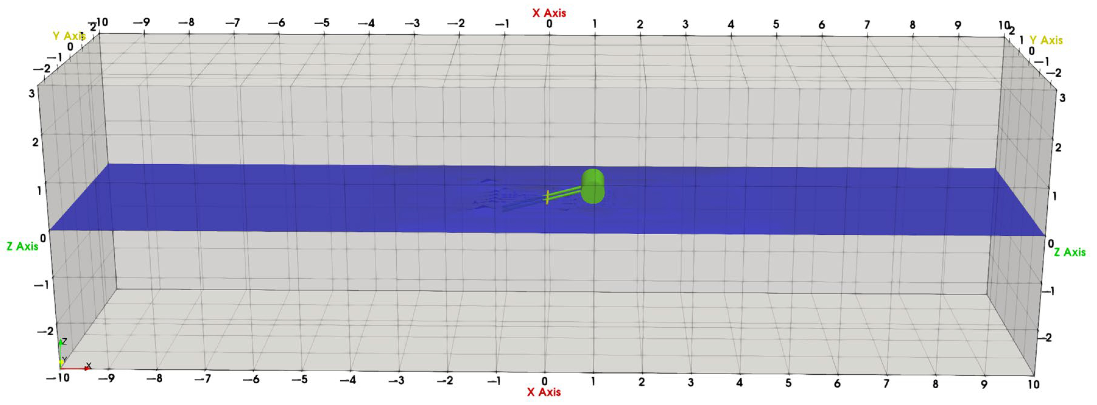
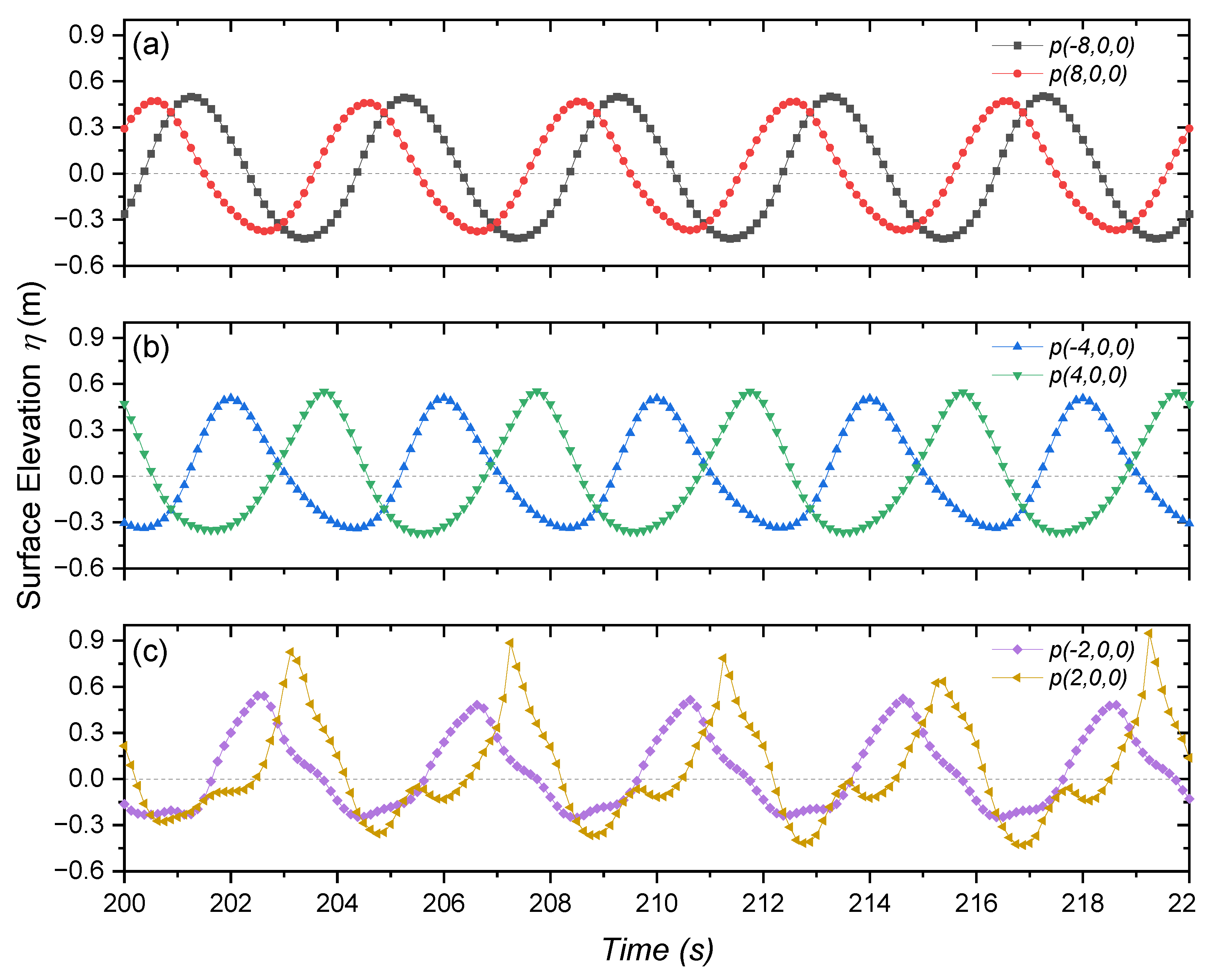
It is also important to analyze the behavior of the surface elevation in different parts of the NWT, since a wave’s shape is a good indicator of non-linear transfers of energy, which could have significant effects on sediment transport close to the shore. Surface elevation time series at different positions of the NWT are presented in Figure 9 and Figure 10. The wave gauge positions, $G_i\left[x\right]$, where $x$ is in the direction of the wave propagation, were established every meter from −10 to 10 m in the $x$ direction, e.g., the third gauge (from left to right); $G_3$ or $G_3\left[-8\right]$ is in position $x=-8$ m. The position of the WEC was at $x=0$, with negative values to the left and positive to the right. All gauges were placed at the still water level. The free surface records for $R=0.25 \mathrm{m}$ and T = 4 s are presented in Figure 9. The gauges in the figure were symetrically selected before ($x=-8,-4,-2$) and after ($x=2, 4, 8$) the buoy’s position. The free surface deformation in gauges $G_9\left[-2\right]$ and $G_{13}\left[2\right]$ was due to the interaction of the waves with the buoy. 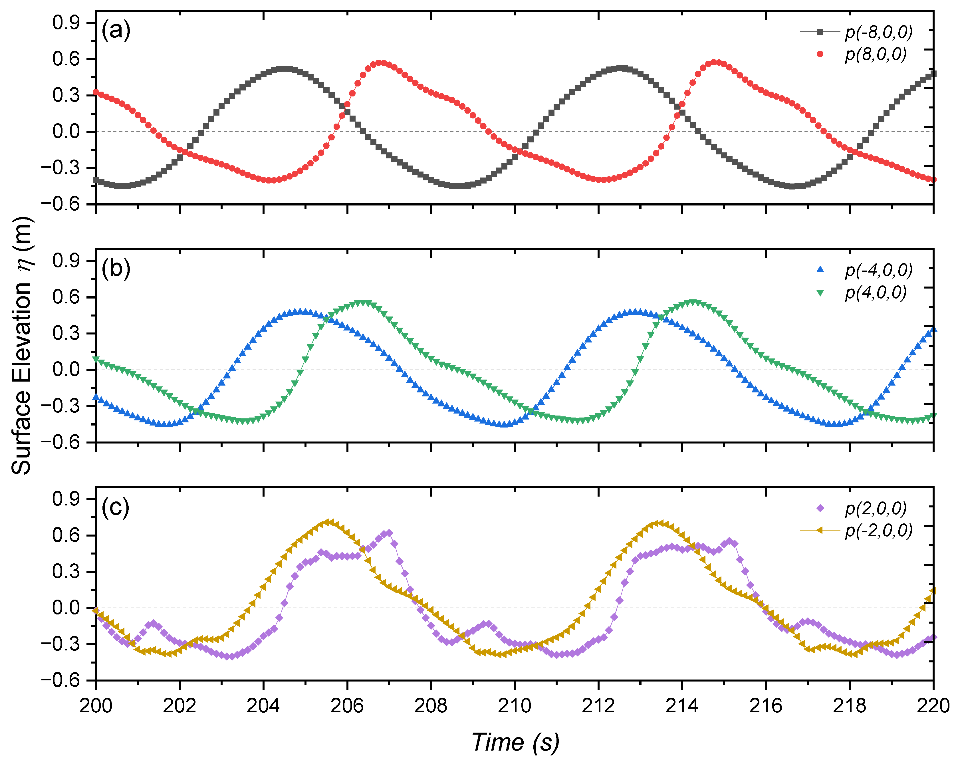Figure 10 shows the same, but for T = 8 s. Several studies have investigated free surface elevation with OpenFOAM, e.g., Zheng et al. compared the maximum crest elevation to both the first- and second-order Stokes theories, showing that the wave elevation predicted by the OpenFOAM simulation and the theory agree well [53].

Figure 9a shows a fairly symmetrical wave record for the waves at the offshore-end of the buoy, which become increasingly skewed (horizontal asymmetry) with the waves at $x=2$ m, the ones having the greatest deformation. The waves on the right-hand side of the NWT gradually recovered their sinusoidal shape, but with less height. For T = 8 s waves (Figure 10), the surface elevation profile starts by presenting less horizontal asymmetry, and the deformations observed closer to the buoy are less pronounced than those observed for T = 4 s. On the right-hand side of the NWT, the waves develop a vertical asymmetry of an inverse saw-tooth shape, which is clearer in the waves farthest from the buoy, at $x=8 \mathrm{m}$.

A more quantitative assessment of the waves’ shape can be performed by calculating the skewness and asymmetry of the waves. As these are associated with processes of sediment transport, the variable used for their evaluation was the near-bottom orbital velocity, rather than surface elevation. Skewness ($S_k$) is related to a horizontal asymmetry in the velocity shape, where the onshore directed orbital velocities are greater and of a shorter duration than the offshore directed orbital velocities, which are milder and of a longer duration (‘Stokes wave’, e.g., Figure 10c for $x=2$). This behaviour of the orbital velocities has been associated with prevailing onshore sediment transport [11,43,54]. Onshore transport is also linked to vertical asymmetry ($A_s$), where waves are pitched forward with a saw-tooth shape (e.g., Figure 10a for $x=8$ shows an inverse saw-tooth shape). Positive values of $A_s$, as defined by Equation (15), are associated with an onshore sediment transport contribution.

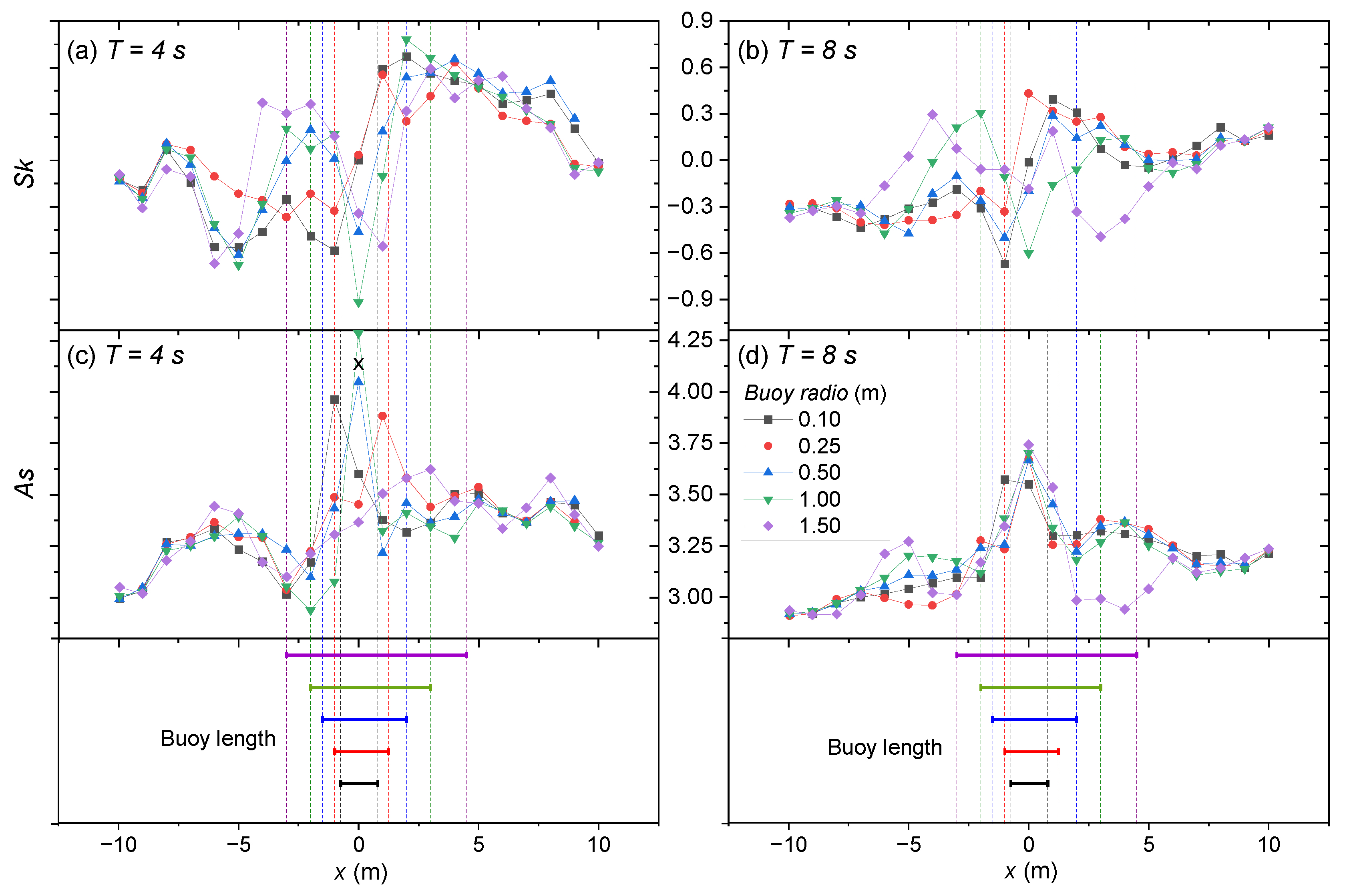
The values of skewness and asymmetry, as calculated using Equations (14) and (15), are shown in Figure 11. For both wave periods, the values of $S_k$ tended to increase considerably towards the buoy’s position, reaching a maximum value just after passing the buoy. From that point, $S_k$ values decreased considerably to values close to 0.1, then increased again towards the end of the NWT. In the case of T = 8 s waves, after passing the buoy, the increase in $S_k$ was less prominent and attained values that were very similar to those reached at the buoy’s position. This tendency can be observed for all the buoys’ radii, implying that the increased onshore sediment transport would alleviate coastal erosion and improve beach accretion. The values of skewness were rather low, since the initial wave conditions only included monochromatic first-order Stokes waves.

The behavior of asymmetry ($A_s$) is presented in Figure 11c,d. For this variable, similar results can be seen, with an increase in $A_s$ close to the buoy. However, there are very important differences between T = 4 s and T = 8 s. With the former, the magnitude of the changes in $A_s$ are very mild (increments of only 0.05) and the evolution of $A_s$ is fairly flat, whereas with T = 8 s, increments in $A_s$ are greater (0.15) and have a fairly linear increment towards the end of the NWT. A comparison between $S_k$ and $A_s$ suggest that the changes in $S_k$ would be more likely to transport sediment onshore than those in $A_s$.

5. Conclusions and Recommendations

5.1. Conclusions

Simulations in a numerical wave tank (NWT), performed with the computational fluid dynamics (CFD) model Open FOAM, were performed to analyze the behavior of a wave energy converter (WEC) that included a cylinder buoy with a pivot point as the axis of rotation. The device was tested with different buoy radii to analyze the effect on power absorption when subjected to regular waves (1st-order Stokes theory) with a uniform wave height ($H=1.0 \mathrm{m}$) and periods of 4 and 8 s.

A considerable amount of literature has been published regarding the use of OpenFOAM to model floating objects interacting with fluids; however, little discussion has been found about the AR, AD, ID, and OD coefficients that are related to body motion parameters. Care must be taken when changing these coefficients, since high values can induce instability due to mesh distortion. The sensibility tests performed with a 0.25 m buoy radius exhibited the greatest variation in the values of torque, which can lead to an overestimation of the output power. Nevertheless, the highest percentage of error (SI value) achieved in this study was relatively low (1.25%) and linked to changes in OD. On the other hand, the values of the angular velocity presented very low errors, compensating for the overestimation tendency of the torque when calculating the power. The values adopted for the analysis coincided with those where the power estimates were lower to avoid overestimation (tests P1 and P7).

The most important result, relative to power absorption by the buoy, is that more power is absorbed by buoys with a greater radius, and that, for a given radius, higher-frequency waves (4 s in this case) absorb several times more power than lower frequency waves (8 s). The power absorbed increases exponentially with the buoy’s radius. The type of WEC device analyzed here performed much better for steep high-frequency waves. The results also show that, for a fixed capture efficiency, shorter-frequency waves need much smaller buoy radii than longer-frequency waves, making the manufacturing process more economically competitive at sites where shorter-frequency waves predominate. The technological development of point-absorber wave energy devices is increasingly close to being economically viable [55]. The results obtained by [51] are similar to those reported here.

This type of device could also serve as an aid to coastal protection if the WEC arrays are properly designed. Not only is energy absorption/dissipation achieved by the obstacle, as observed by the low-transmission coefficients, but also due to the transformations that the buoy induces on the nonlinear properties of the wave field, such as wave skewness and asymmetry. Skewness values increased considerably at the position of the buoy and further onshore, suggesting that the devices could induce onshore sediment transport.

As it was not possible to evaluate all cases with complex geometries at a high resolution in this research, the NWT was set up with a coarse mesh. However, instead of changing the mesh density, the most critical scenario was evaluated after numerical sensitive tests, in order not to overestimate the result.

5.2. Recommendations

These results should be treated with caution as there are no full-scale laboratory results that can be used to validate the results of the numerical model. Therefore, it is recommended to verify the consistency of these numerical results using a much finer mesh and, thus, perhaps improve the accuracy and stability of the numerical simulations. When objects in movement are included in the simulation, it is important to consider the parameters of inner and outer distances. Although the torque values were included in the numerical results, the effect of the hydrodynamic forces needs to be considered, as it has a direct relation with the ratio of the arm and radii of the buoy.

When modeling the buoy as a breakwater, an important parameter is the relative length of the buoy, which determines the amount of wave energy reflected. However, since the buoy has a degree of freedom, the change in the relative length could be misleading; a suitable alternative methodology has been described [56], in which the individual parameters are closely related to each other [57].

Finally, related to onshore sediment transport, further analyses are needed to understand these effects under spectral wave fields and with larger buoy configurations, which are beyond the scope of this research.

References

1. Gunn, K.; Stock-Williams, C. Quantifying the global wave power source. Renew. Energy 2012, 44, 296–304. [Google Scholar] [CrossRef]
2. Polinder, H.; Scuotto, M. Wave energy converters and their impact on power systems. In Proceedings of the 2005 International Conference on Future Power Systems, Amsterdam, The Netherlands, 18 November 2005; Available online: https://ieeexplore.ieee.org/document/1600483 (accessed on 27 March 2023).
3. Henriques, J.C.C.; Gato, L.M.C.; Falcao, A.F.O.; Robles, E.; Fay, F.X. Latching control of a floating oscillating-water-column wave energy converter. Renew. Energy 2016, 90, 229–241. [Google Scholar] [CrossRef]
4. Esmaeilzadeh, S.; Alam, M.R. Shape optimization of wave energy converters for broadband directional incident waves. Ocean Eng. 2019, 174, 186–200. [Google Scholar] [CrossRef]
5. Garcia-Teruel, A.; Forehand, D.I.M. A review of geometry optimisation of wave energy converters. Renew. Sustain. Energy Rev. 2021, 139, 110593. [Google Scholar] [CrossRef]
6. Trapani, K.; Millar, D.L.; Smith, H.C.M. Novel offshore application of photovoltaics in comparison to conventional marine renewable energy technologies. Renew. Energy 2013, 50, 879–888. [Google Scholar] [CrossRef]
7. Dalton, G.J.; Alcorn, R.; Lewis, T. Case study feasibility analysis of the Pelamis wave energy convertor in Ireland, Portugal and North America. Renew. Energy 2010, 35, 443–455. [Google Scholar] [CrossRef]
8. The European Marine Energy Centre LTD. Press Release: Council Takes Ownership of Pelamis Device, 6 July 2017. Available online: http://www.emec.org.uk/press-release-council-takes-ownership-of-pelamis-device/ (accessed on 27 March 2023).
9. The European Marine Energy Centre LTD. Aquamarine Power. Available online: http://www.emec.org.uk/about-us/wave-clients/aquamarine-power/ (accessed on 27 March 2023).
10. Carnegie Clean Energy. CETO 5-Perth (WA). Available online: https://www.carnegiece.com/portfolio/ceto-5-perth-wa/ (accessed on 27 March 2023).
11. Hoefel, F.; Elgar, S. Wave-Induced Sediment Transport and Sandbar Migration. Science 2003, 299, 1885–1887. [Google Scholar] [CrossRef]
12. Astariz, S.; Iglesias, G. The economics of wave energy: A review. Renew. Sustain. Energy Rev. 2015, 45, 397–408. [Google Scholar] [CrossRef]
13. Teixeira-Duarte, F.; Clemente, D.; Gianini, G.; Rosa-Santos, P.; Taveira-Pinto, F. Review on layout optimization strategies of offshore parks for wave energy converters. Renew. Sustain. Energy Rev. 2022, 163, 112513. [Google Scholar] [CrossRef]
14. Karan, H.; Thomson, R.C.; Harrison, G.P. Full life cycle assessment of two surge wave energy converters. Proc. IMechE Part A J. Power Energy 2020, 234, 548–561. [Google Scholar] [CrossRef]
15. Nasrollahi, S.; Kazemi, A.; Jahangir, M.-H.; Aryaee, S. Selecting suitable wave energy technology for sustainable development, an MCDM approach. Renew. Energy 2023, 202, 756–772. [Google Scholar] [CrossRef]
16. Foteinis, S. Wave energy converters in low energy seas: Current state and opportunities. Renew. Sustain. Energy Rev. 2022, 162, 112448. [Google Scholar] [CrossRef]
17. Xu, R.; Wang, H.; Xi, Z.; Wang, W.; Xu, M. Recent progress on wave energy marine buoys. J. Mar. Sci. Eng. 2022, 10, 566. [Google Scholar] [CrossRef]
18. Falnes, J.; Kurniawan, A. Ocean Waves and Oscillating Systems: Linear Interactions Including Wave-Energy Extraction; Cambridge University Press: Cambridge, UK, 2020; Volume 8. [Google Scholar]
19. Greenshields, C.J. OpenFOAM User Guide Version 5.0; The OpenFOAM Foundation: London, UK, 2015; p. 47. [Google Scholar]
20. Windt, C.; Davidson, J.; Ringwood, J.V. High-fidelity numerical modelling of ocean wave energy systems: A review of computational fluid dynamics-based numerical wave tanks. Renew. Sustain. Energy Rev. 2018, 93, 610–630. [Google Scholar] [CrossRef]
21. Giorgi, G.; Penalba Retes, M.; Ringwood, J.V. Nonlinear Hydrodynamic Models for Heaving Buoy Wave Energy Converters. In Proceedings of the 3rd Asian Wave and Tidal Energy Conference, Singapore, 2016; Available online: https://tethys-engineering.pnnl.gov/publications/nonlinear-hydrodynamic-models-heaving-buoy-wave-energy-converters (accessed on 27 March 2023).
22. Windt, C.; Davidson, J.; Akram, B.; Ringwood, J.V. Performance assessment of the overset grid method for numerical wave tank experiments in the OpenFOAM environment. In Proceedings of the 37th International Conference on Ocean, Offshore and Arctic Engineering, Madrid, Spain, 17–22 June 2018; American Society of Mechanical Engineers: Madrid, Spain, 2018. [Google Scholar]
23. Davidson, J.; Karimov, M.; Szelechman, A.; Windt, A.; Ringwood, J. Dynamic mesh motion in OpenFOAM for wave energy converter simulation. In Proceedings of the 14th OpenFOAM Workshop, Duisburg, Germany, 23–26 July 2019. [Google Scholar] [CrossRef]
24. Windt, C.; Davidson, J.; Chandar, D.D.J.; Faedo, N.; Ringwood, J.V. Evaluation of the overset grid method for control studies of wave energy converters in OpenFOAM numerical wave tanks. J. Ocean Eng. Mar. Energy 2020, 6, 55–70. [Google Scholar] [CrossRef]
25. Windt, C.; Davidson, J.; Chandar, D.; Ringwood, J.V. On the importance of advanced mesh motion methods for WEC experiments in CFD-based numerical wave tanks. In Proceedings of the VIII International Conference on Computational Methods in Marine Engineering, CIMNE, Gothenburg, Sweden, 13–15 May 2019; pp. 145–156. Available online: https://www.semanticscholar.org/paper/On-the-Importance-of-Advanced-Mesh-Motion-Models-in-Windt-Davidson/4db8059cbaa4e7a2ac56bfaf9df16da4f3e339e6 (accessed on 27 March 2023).
26. OpenFOAM. 6.2 Numerical Schemes. Available online: https://www.openfoam.com/documentation/user-guide/6-solving/6.2-numerical-schemes (accessed on 29 March 2023).
27. Devolder, B.; Schmitt, P.; Rauwoens, P.; Elsaesser, B.; Troch, P. A review of the implicit motion solver algorithm in OpenFOAM® to simulate a heaving buoy. In Proceedings of the 18th Numerical Towing Tank Symposium, Cortona, Italy, 2015; Available online: https://www.semanticscholar.org/paper/A-Review-of-the-Implicit-Motion-Solver-Algorithm-in-Devolder-Schmitt/cf5ec01ae9176fe20a4a732840e320c5a58e08cc (accessed on 27 March 2023).
28. Holzmann, T. Mathematics, numerics, derivations and OpenFOAM®. In The Basics for Numerical Simulations; Holzman CFD: Loeben, Germany, 2016. [Google Scholar]
29. Chow, J.H.; Ng, E.Y.K. Strongly coupled partitioned six degree-of-freedom rigid body motion solver with Aitken’s dynamic under-relaxation. Int. J. Nav. Archit. Ocean. Eng. 2016, 8, 320–329. [Google Scholar] [CrossRef]
30. SALOME, The Open Source Integration Platform for Numerical Simulation. Available online: https://www.salome-platform.org/ (accessed on 29 March 2023).
31. Jacobsen, N.G. waves2Foam Manual; Deltares: Delft, The Netherlands, 2017. [Google Scholar]
32. Dhanak, M.R.; Xiros, N.I. (Eds.) Springer Handbook of Ocean Engineering; Springer: Berlin/Heidelberg, Germany, 2016. [Google Scholar]
33. Budar, K.; Falnes, J. A resonant point absorber of ocean-wave power. Nature 1975, 256, 478–479. [Google Scholar] [CrossRef]
34. Evans, D.V. A theory for wave-power absorption by oscillating bodies. J. Fluid Mech. 1976, 77, 1–25. [Google Scholar] [CrossRef]
35. Falcao, A. Wave energy utilization: A review of the technologies. Renew. Sustain. Energy Rev. 2010, 14, 899–918. [Google Scholar] [CrossRef]
36. Babarit, A. Ocean Wave Energy Conversion: Resource, Technologies and Performance; Elsevier: Amsterdam, The Netherlands, 2017. [Google Scholar]
37. Babarit, A. A database of capture width ratio of wave energy converters. Renew. Energy 2015, 80, 610–628. [Google Scholar] [CrossRef]
38. Abanades, J.; Greaves, D.; Iglesias, G. Wave farm impact on the beach profile: A case study. Coast. Eng. 2014, 86, 36–44. [Google Scholar] [CrossRef]
39. Loukili, M.; Dutykh, D.; Pincemin, S.; Kotrasova, K.; Abcha, N. Theoretical Investigation Applied to Scattering Water Waves by Rectangular Submerged Obstacles/and Submarine Trenches. Geosciences 2022, 12, 379. [Google Scholar] [CrossRef]
40. Seelig, W.N.; Ahrens, J.P. Estimation of Wave Reflection and Energy Dissipation Coefficients for Beaches, Revetments, and Breakwaters; Coastal Engineering Research Center: Fort Belvoir, Virginia, 1981. [Google Scholar]
41. Mansard, E.P.D.; Funke, E.R. The measurement of incident and reflected spectra using a least squares method. In Proceedings of the 17th International Conference on Coastal Engineering, Sydney, Australia, 23–28 March 1980; pp. 154–172. Available online: https://repository.tudelft.nl/islandora/object/uuid%3A840a64af-b113-4372-8f91-47b4d7a3cc78 (accessed on 27 March 2023).
42. Atan, R.; Finnegan, W.; Nash, S.; Goggins, J. The effect of arrays of wave energy converters on the nearshore wave climate. Ocean Eng. 2019, 172, 373–384. [Google Scholar] [CrossRef]
43. Fernández-Mora, A.; Calvete, D.; Falqués, A.; de Swart, H.E. Onshore sandbar migration in the surf zone: New insights into the wave-induced sediment transport mechanisms. Geophys. Res. Lett. 2015, 42, 2869–2877. [Google Scholar] [CrossRef]
44. Berni, C.; Barthélemy, E.; Michallet, H. Surf zone cross-shore boundary layer velocity asymmetry and skewness: An experimental study on a mobile bed. J. Geophys. Res. Oceans 2013, 118, 2188–2200. [Google Scholar] [CrossRef]
45. Gao, J.-L.; Lyu, J.; Zhang, J.; Liu, Q.; Zang, J.; Zou, T. Study on Transient Gap Resonance with Consideration of the Motion of Floating Body. China Ocean Eng. 2022, 36, 994–1006. [Google Scholar] [CrossRef]
46. Gao, J.; He, Z.; Huang, X.; Liu, Q.; Zang, J.; Wang, G. Effects of free heave motion on wave resonance inside a narrow gap between two boxes under wave actions. Ocean Eng. 2021, 224, 108753. [Google Scholar] [CrossRef]
47. Qu, S.; Liu, S.; Ong, M.C.; Wang, X.; Sun, S. Numerical simulation of free-surface waves past semi-submerged two-dimensional rectangular prisms with different aspect ratios and rounding chamfer radii. Ocean Eng. 2023, 269, 113604. [Google Scholar] [CrossRef]
48. Wang, K.; Ma, X.; Bai, W.; Lin, Z.; Li, Y. Numerical simulation of water entry of a symmetric/asymmetric wedge into waves using OpenFOAM. Ocean Eng. 2021, 227, 108923. [Google Scholar] [CrossRef]
49. Palm, J.; Eskilsson, C.; Moura Paredes, G.; Bergdahl, L. Coupled mooring analysis for floating wave energy converters using CFD: Formulation and validation. Int. J. Marine Energy 2016, 16, 83–99. [Google Scholar] [CrossRef]
50. Loh, T.T.; Pizer, D.; Simmonds, D.; Kyte, A.; Greaves, D. Simulation and analysis of wave-structure interactions for a semi-immersed horizontal cylinder. Ocean Eng. 2018, 147, 676–689. [Google Scholar]
51. Diaz-Maya, M.; Ulloa, M.; Silva, R. Assessing wave energy converters in the gulf of Mexico using a multi-criteria approach. Front. Energy Res. 2022, 10, 929625. [Google Scholar] [CrossRef]
52. Dai, J.; Wang, C.M.; Utsunomiya, Y.; Duan, W. Review of recent research and developments on floating breakwaters. Ocean Eng. 2018, 158, 132–151. [Google Scholar] [CrossRef]
53. Hu, Z.Z.; Greaves, D.; Raby, A. Numerical wave tank study of extreme waves and wave-structure interaction using OpenFoam®. Ocean Eng. 2016, 126, 329–342. [Google Scholar] [CrossRef]
54. Elgar, S.; Guza, R.T.; Freilich, M.H. Eulerian measurements of horizontal accelerations in shoaling gravity waves. J. Geophys. Res. Oceans 1988, 93, 9261–9269. [Google Scholar] [CrossRef]
55. Al Shami, E.; Zhang, R.; Wang, X. Point absorber wave energy harvesters: A review of recent developments. Energies 2018, 12, 47. [Google Scholar] [CrossRef]
56. Loukili, M.; Dutykh, D.; Hadjib, C.; Ning, D.; Kotrasova, K. Analytical and Numerical Investigations Applied to Study the Reflections and Transmissions of a Rectangular Breakwater Placed at the Bottom of a Wave Tank. Geosciences 2021, 11, 430. [Google Scholar] [CrossRef]
57. Ozkop, E.; Altas, I.H. Control, power and electrical components in wave energy conversion systems: A review of the technologies. Renew. Sustain. Energy Rev. 2017, 67, 106–115. [Google Scholar] [CrossRef]
Figure 1. NWT for the simulation with a buoy with a 0.25 m radius (R). Wave propagation is in the direction of the positive x-axis, the free surface elevation coincides with the z direction, and the length of the buoy is in the y direction. The wave gauges are placed from −10 to 10 in the x direction at y = 0 .
Applsci 13 05182 g001
Figure 2. (a) Buoy with radius R ; B is the characteristic width (1 m) and L b is the arm length, while y is the rotation axis; (b) Top view of the buoy.
Applsci 13 05182 g002
Figure 3. Schematic representation of the cylindrical buoy’s WEC implementation process.
Applsci 13 05182 g003
Figure 4. Comparison of the surface wave elevation ( η ) at the NWT inlet calculated with the theoretical result and simulation: (a) for T = 4   s and (b) for T = 8   s , with H = 1   m in both cases. The NWT considers the R 2 buoy.
Applsci 13 05182 g004
Figure 5. One hundred waves simulated for the buoy with R = 0.25 m: (a) for T = 4 s and (b) for T = 8 s. Details of P1 to P9 are described later in Section 4.2.
Applsci 13 05182 g005
Figure 6. Mean absorbed power and its standard deviation for the sensitivity tests of the cases presented in Table 4 (H = 1.0 m and R = 0.25 m), organized by wave period and the tested parameters.
Applsci 13 05182 g006
Figure 7. Statistical analysis for the center of mass (CofM_Z), angular momentum (Mom_Ang), angular velocity (Vel_Ang), torque, and output power (Pot) for the cases presented in Table 5. (a) Root Mean Square Error (RMSE); (b) Scatter Index (SI); (c) Pearson correlation coefficient (r); (d) underestimation or overestimation tendency (BIAS).
Applsci 13 05182 g007
Figure 8. (a) Average power absorbed by the WEC at different radius sizes for both T = 4 s and T = 8 s wave periods. (b) Capture efficiency per buoy unit length for different values of the normalized buoy diameter (radius/wavelength) for both T = 4 s and T = 8 s wave periods. AR = 0.7, AD = 1, ID = 0.001, and OD = 1.5. ** OD = 2.0.
Applsci 13 05182 g008
Figure 9. Surface elevation records for the test with H = 1.0 m, T = 4 s, and R = 0.25 m for virtual gauges at symmetrical distances from the buoy: (a) 2, (b) 4, and (c) 8 m to each side. Negative values to the left of the buoy and positive to the right.
Applsci 13 05182 g009
Figure 10. Surface elevation records for the test with H = 1.0 m, T = 8 s, and R = 0.25 m for virtual gauges at symmetrical distances from the buoy: (a) 2, (b) 4, and (c) 8 m to each side. Negative values to the left of the buoy and positive to the right.
Applsci 13 05182 g010
Figure 11. Skewness (horizontal asymmetry (a,b) and asymmetry velocity (c,d)) evaluated with five buoys’ radii for T = 4 s and T = 8 s. The different colors represent different buoys’ sizes, as shown in the bottom panels. The vertical, dashed lines show the position of the buoy, with the different colors representing different buoys’ radii.
Applsci 13 05182 g011