

The Contribution of Near-Surface Geophysics for the Site Characterization of Seismological Stations
 , ,
, ,  and
and
Abstract
:1. Introduction
2. Methodology
2.1. Seismic Method
2.1.1. Data
2.1.2. Processing
HVSR Technique
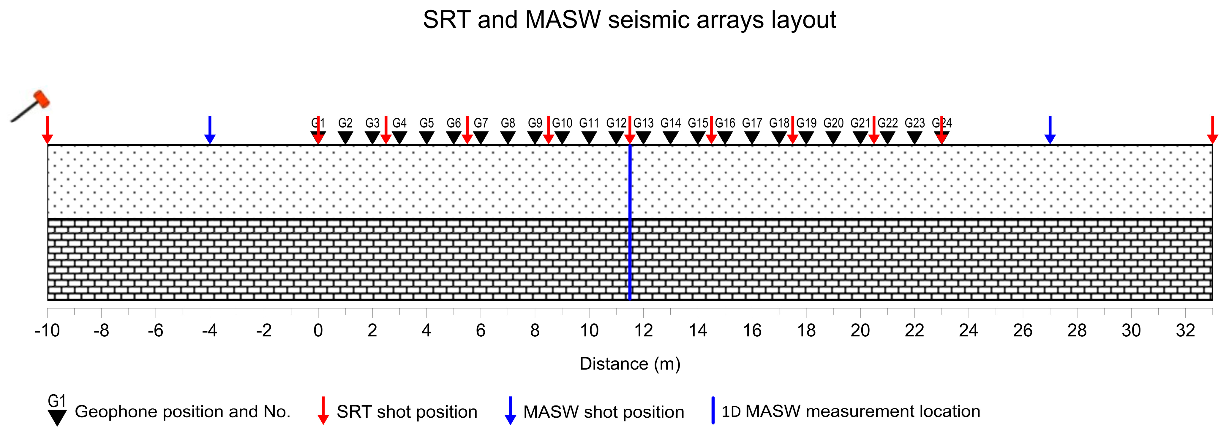
SRT Technique
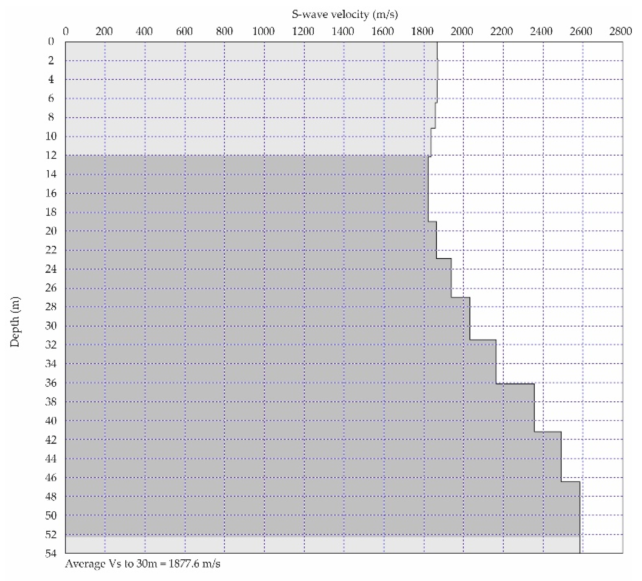
MASW Processing
2.2. Electrical Resistivity Tomography
2.3. Density Determination
3. Application of the Geophysical Surveys and Processing Results
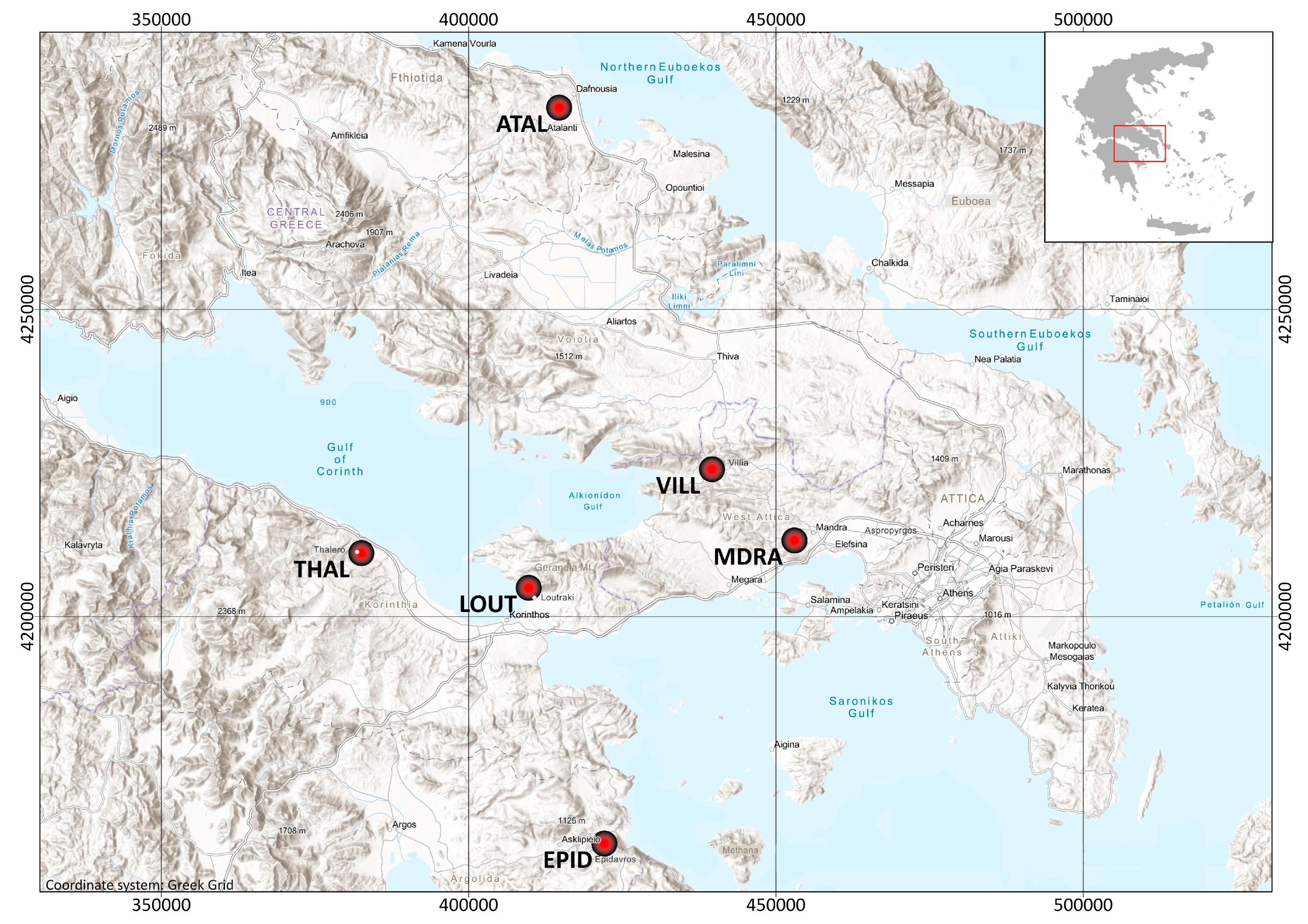
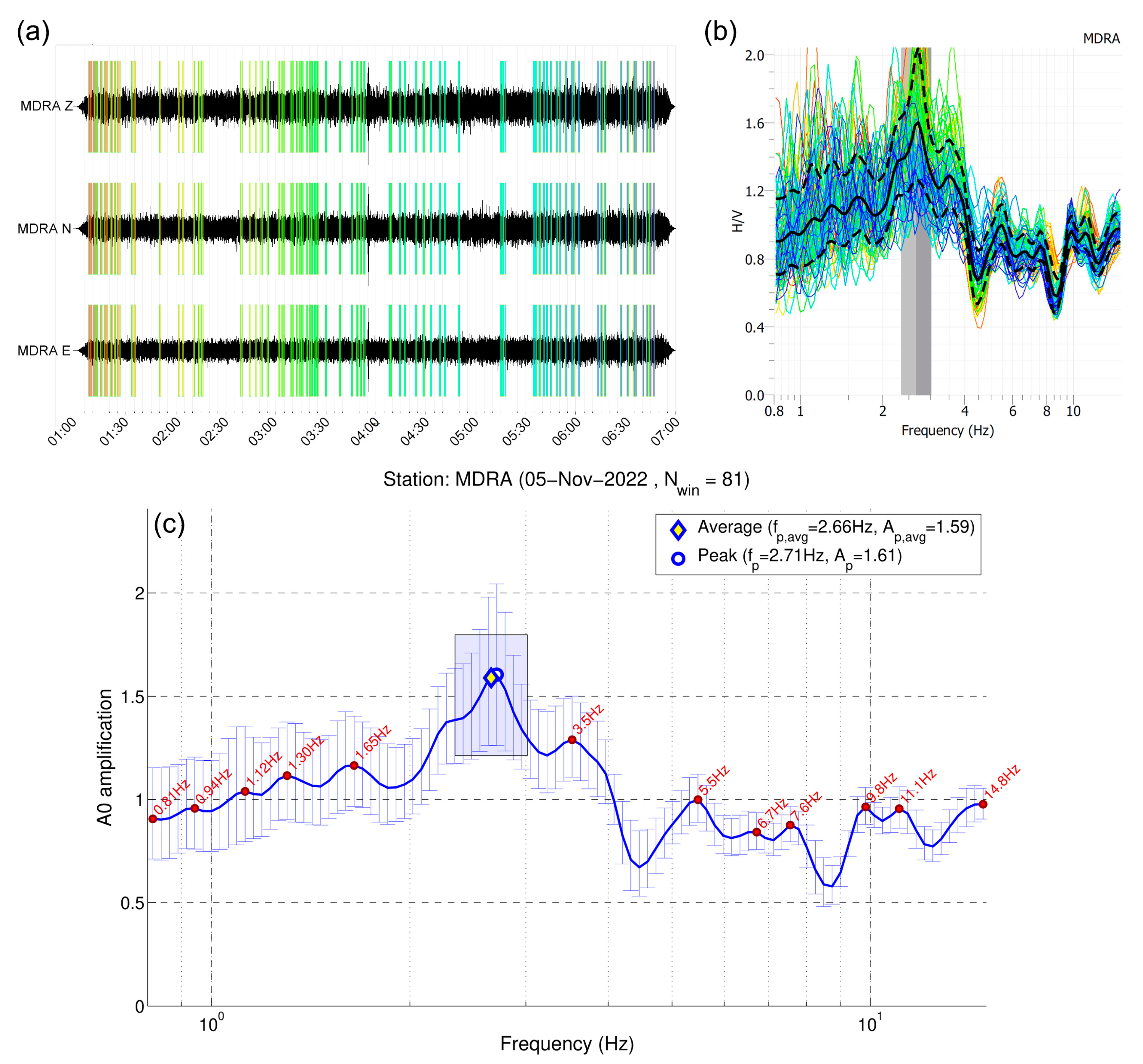
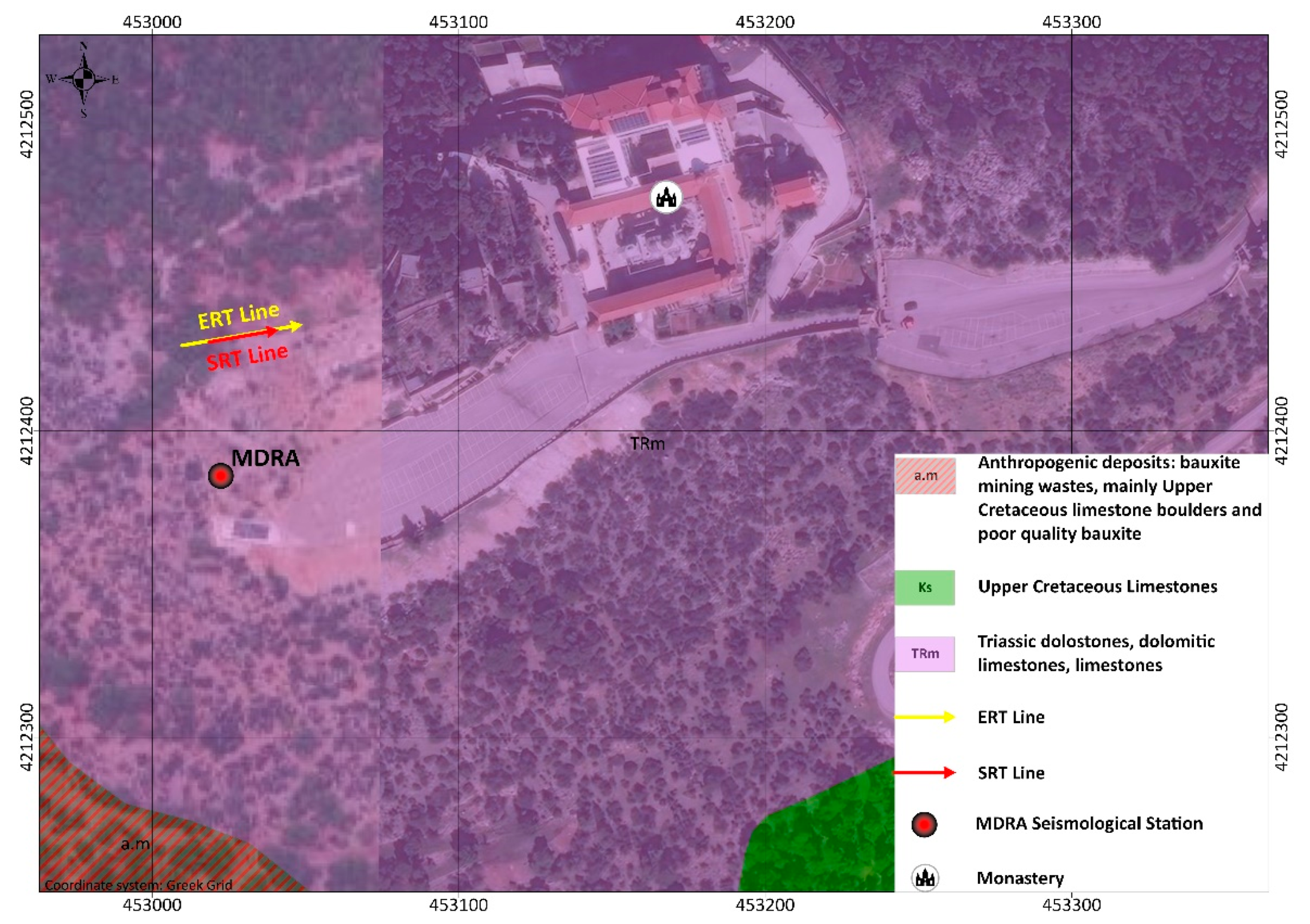
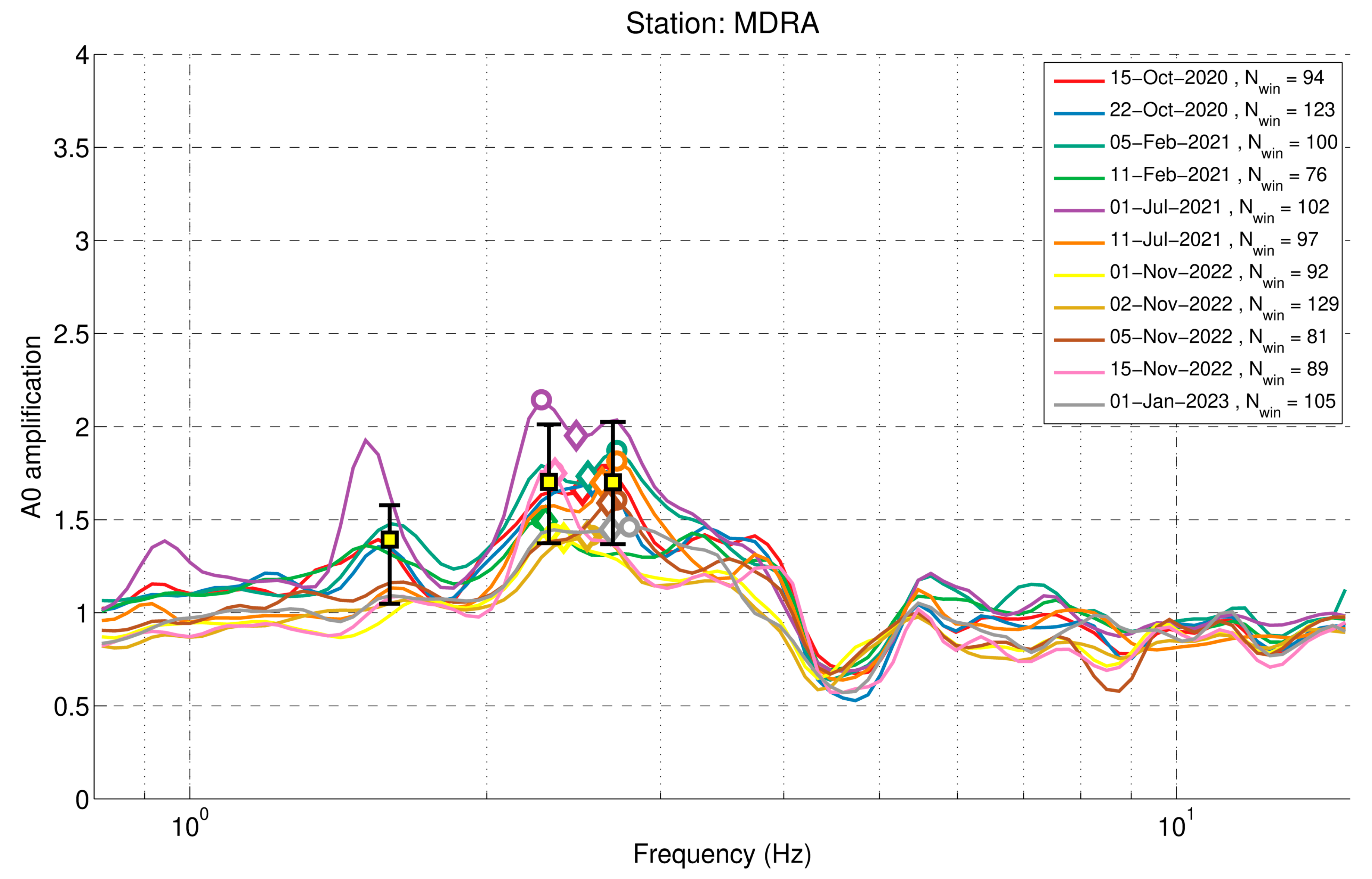
3.1. Seismological Station at Mandra, Attica (MDRA)
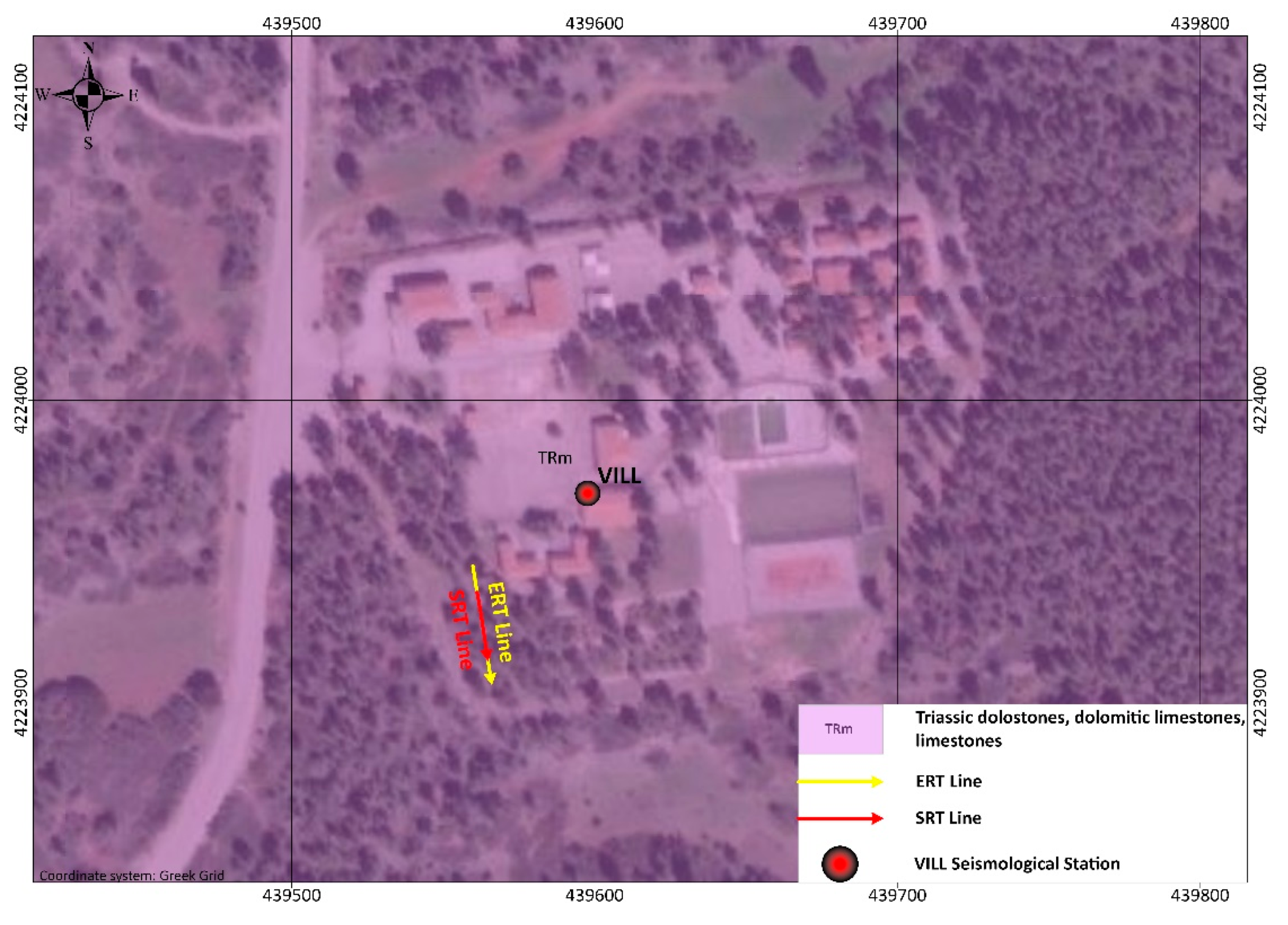
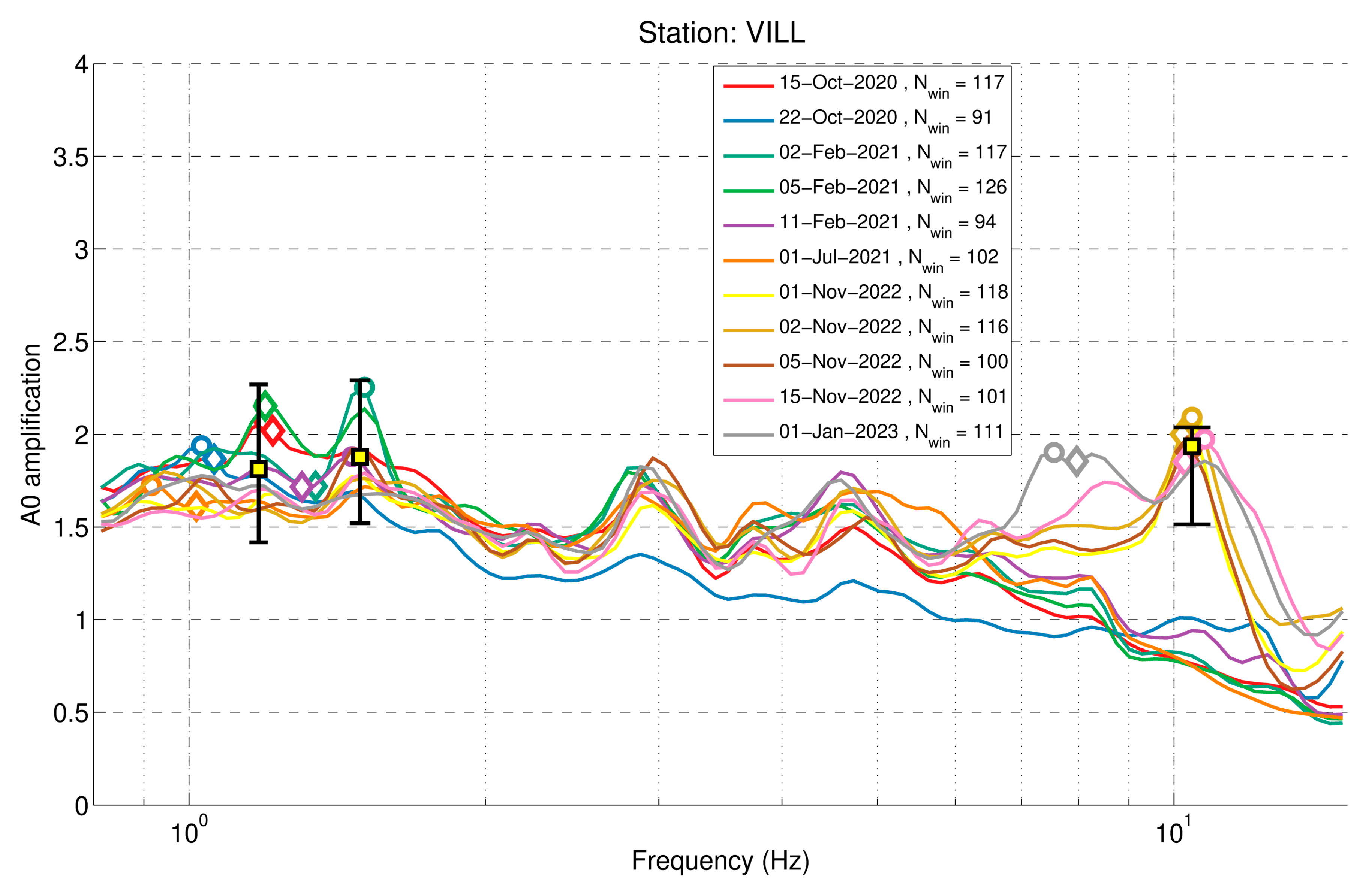
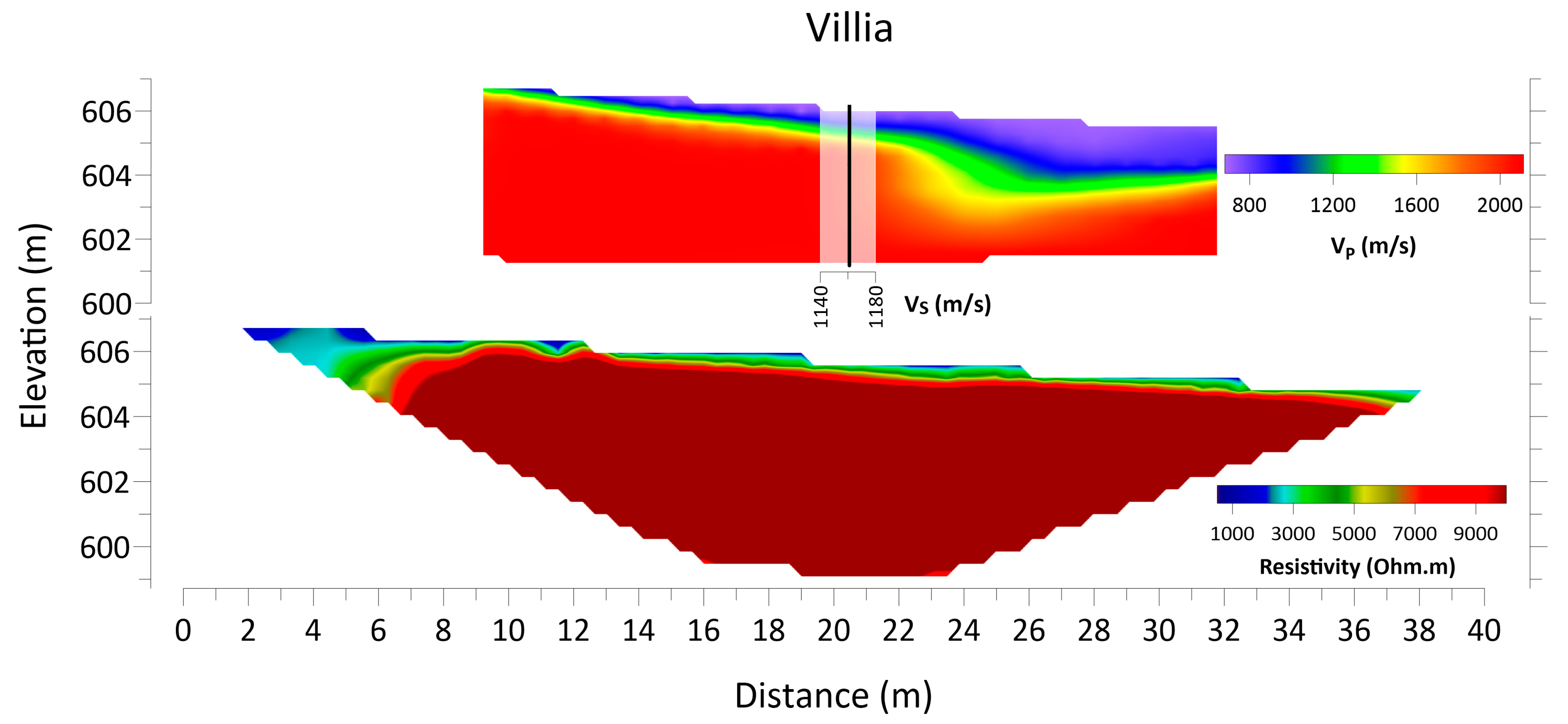
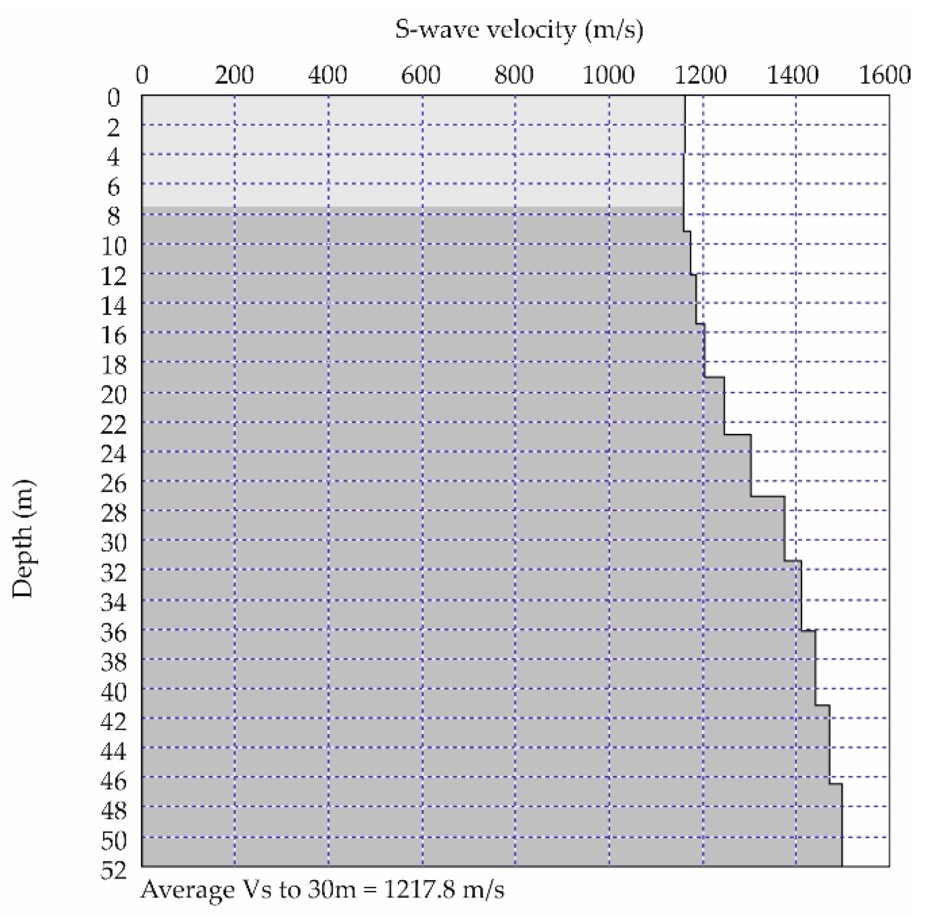
3.2. Seismological Station at Villia, Attica (VILL)
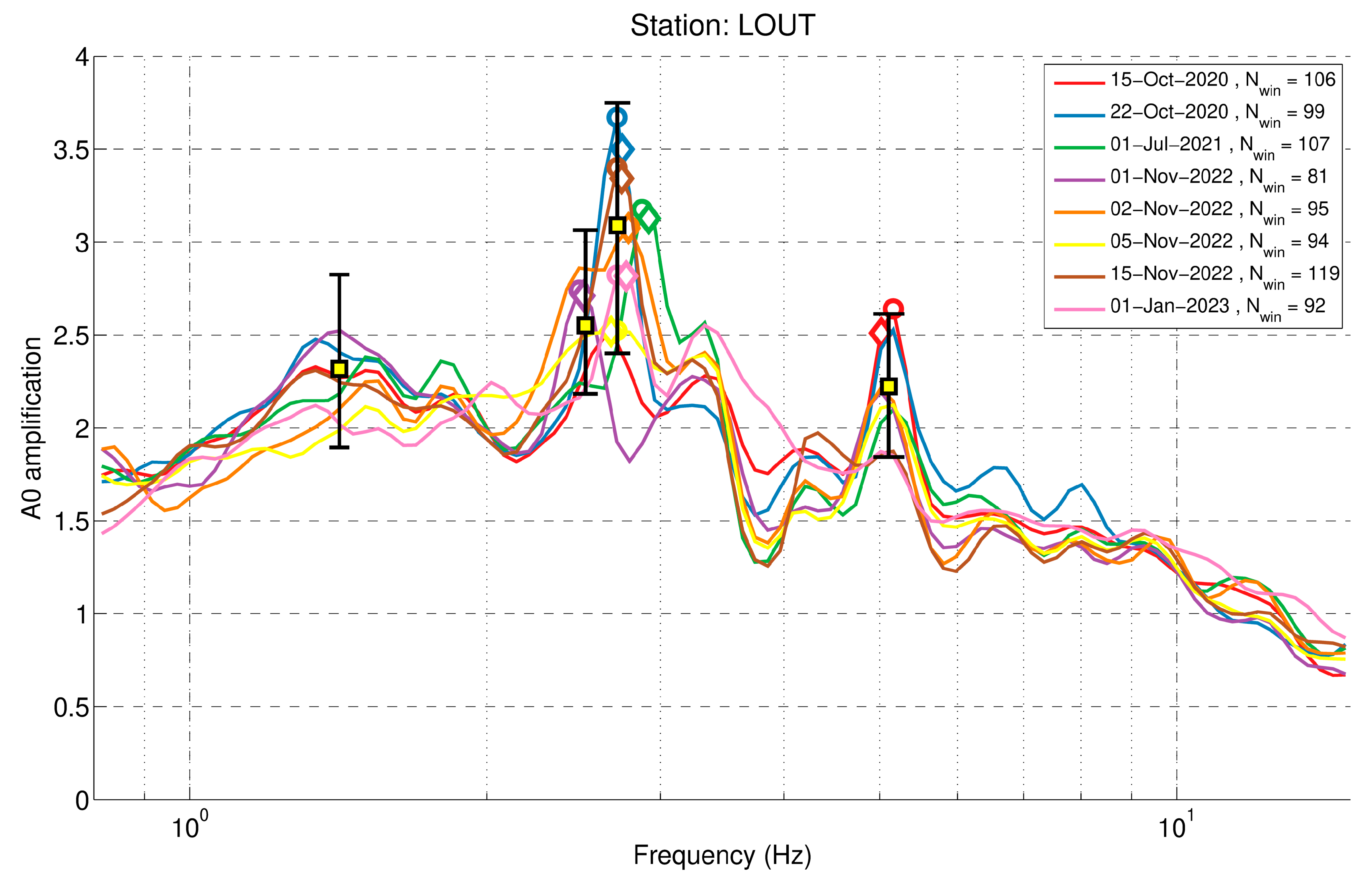
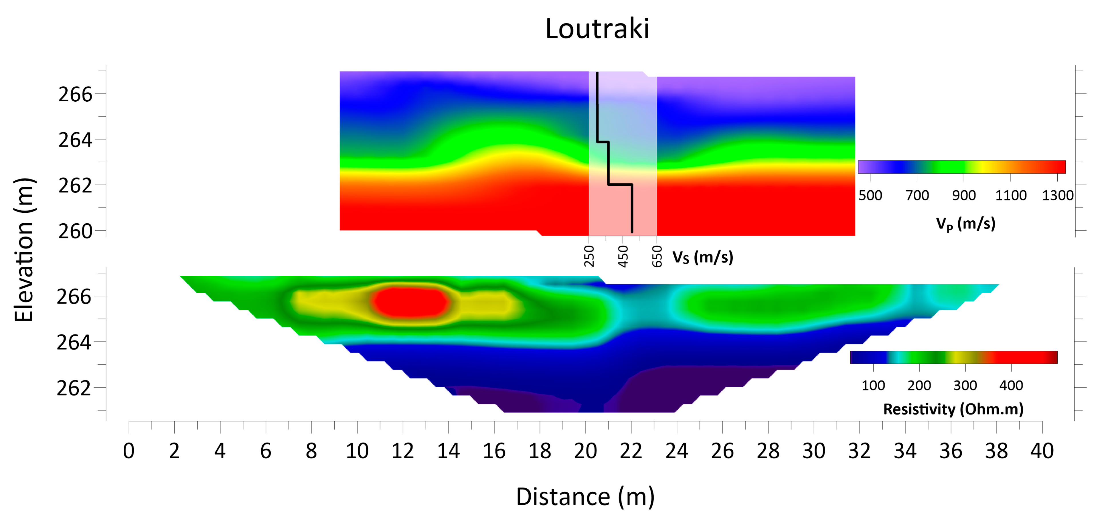
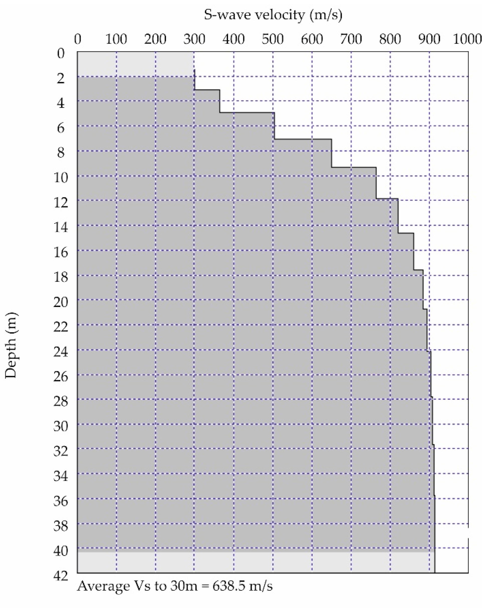
3.3. Seismological Station at Loutraki, Korinthia (LOUT)
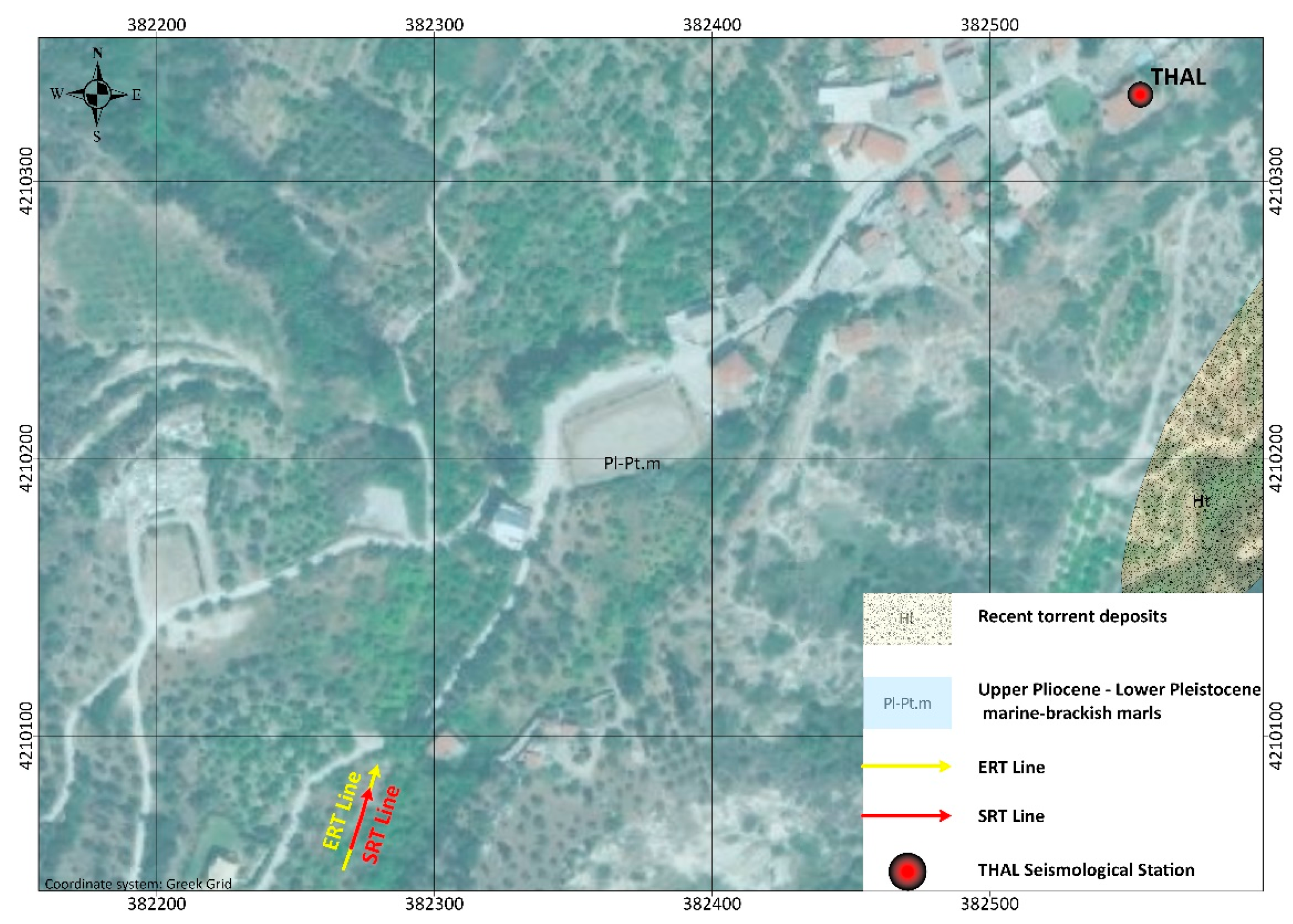
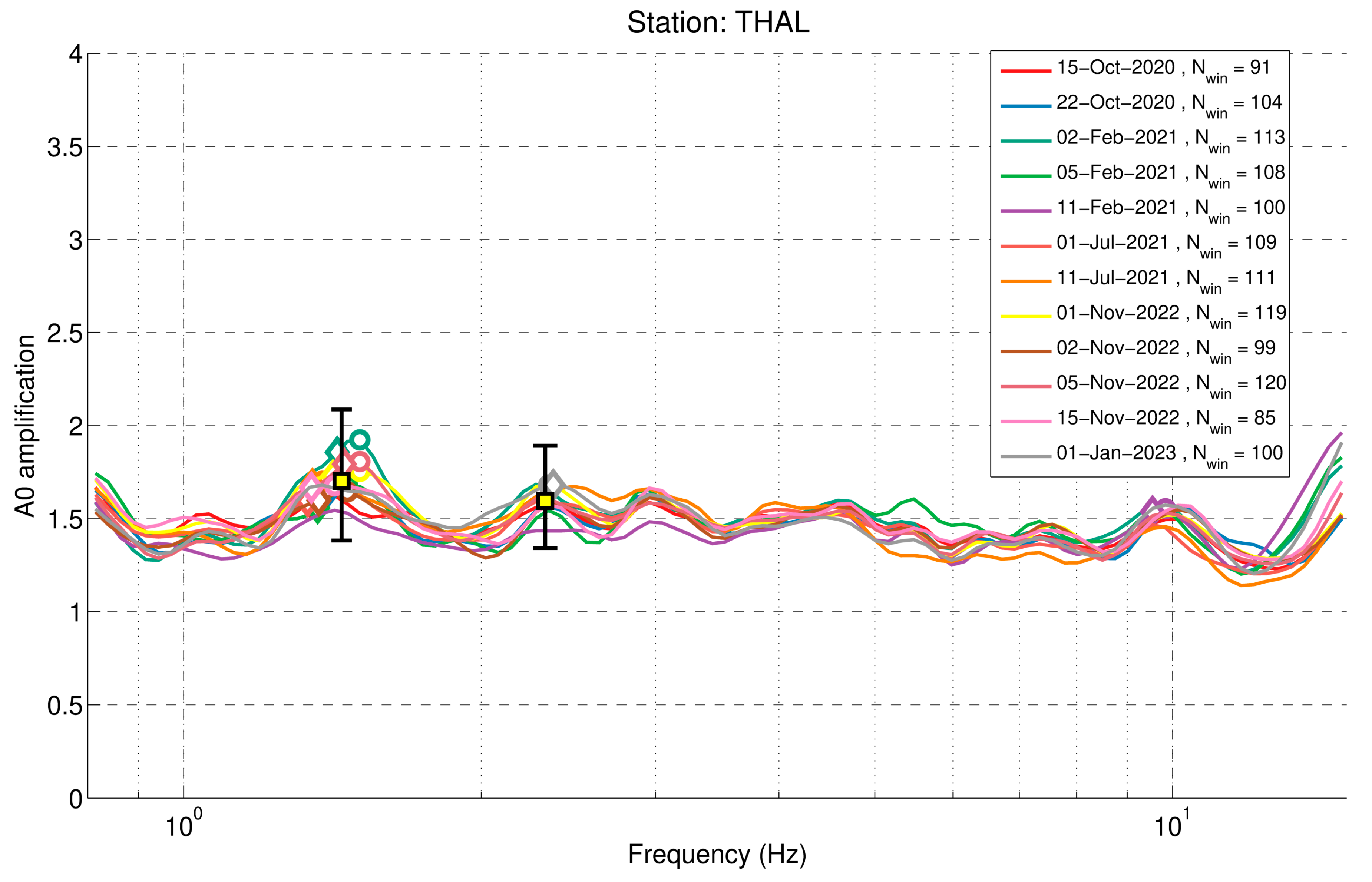
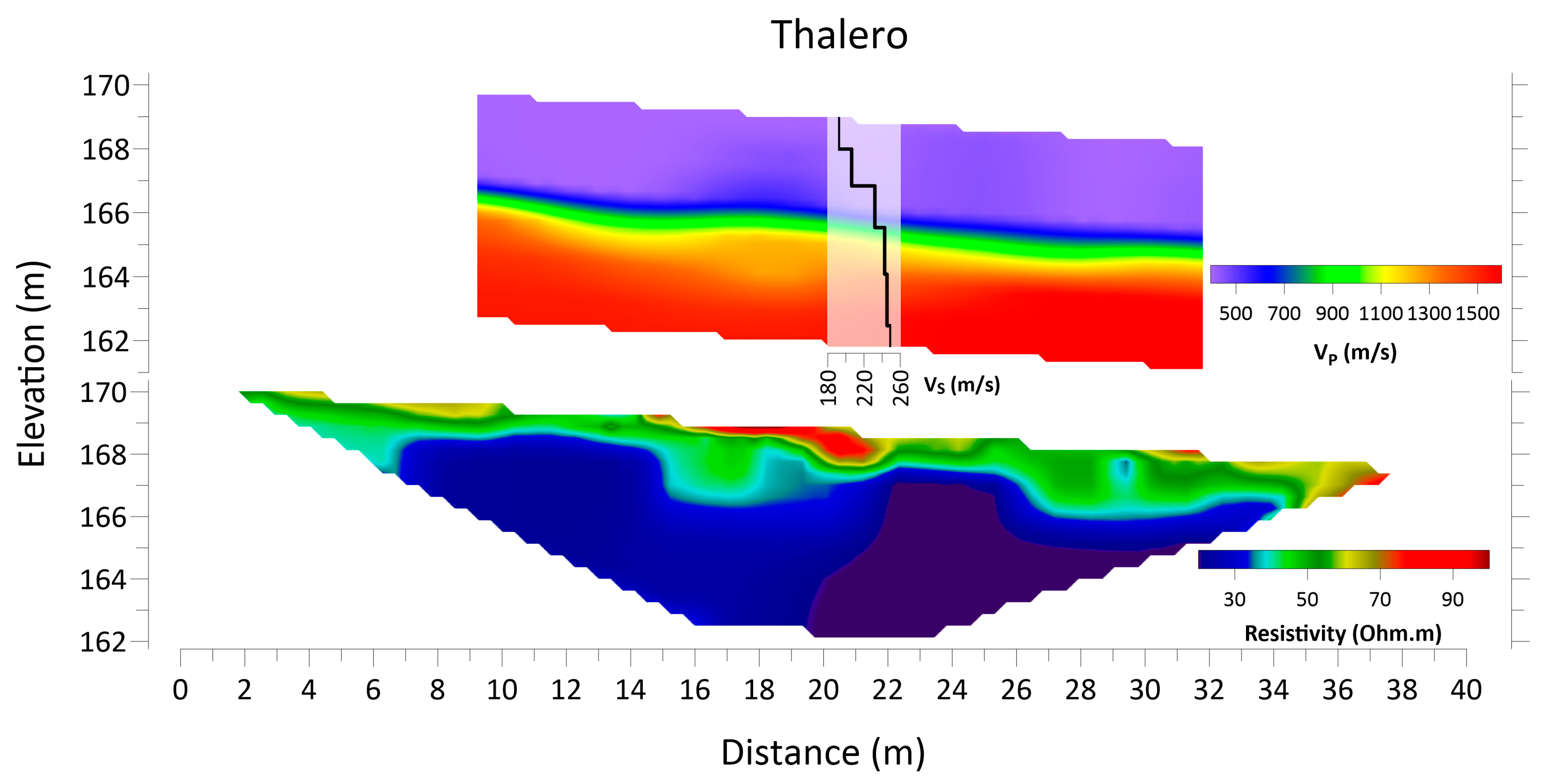
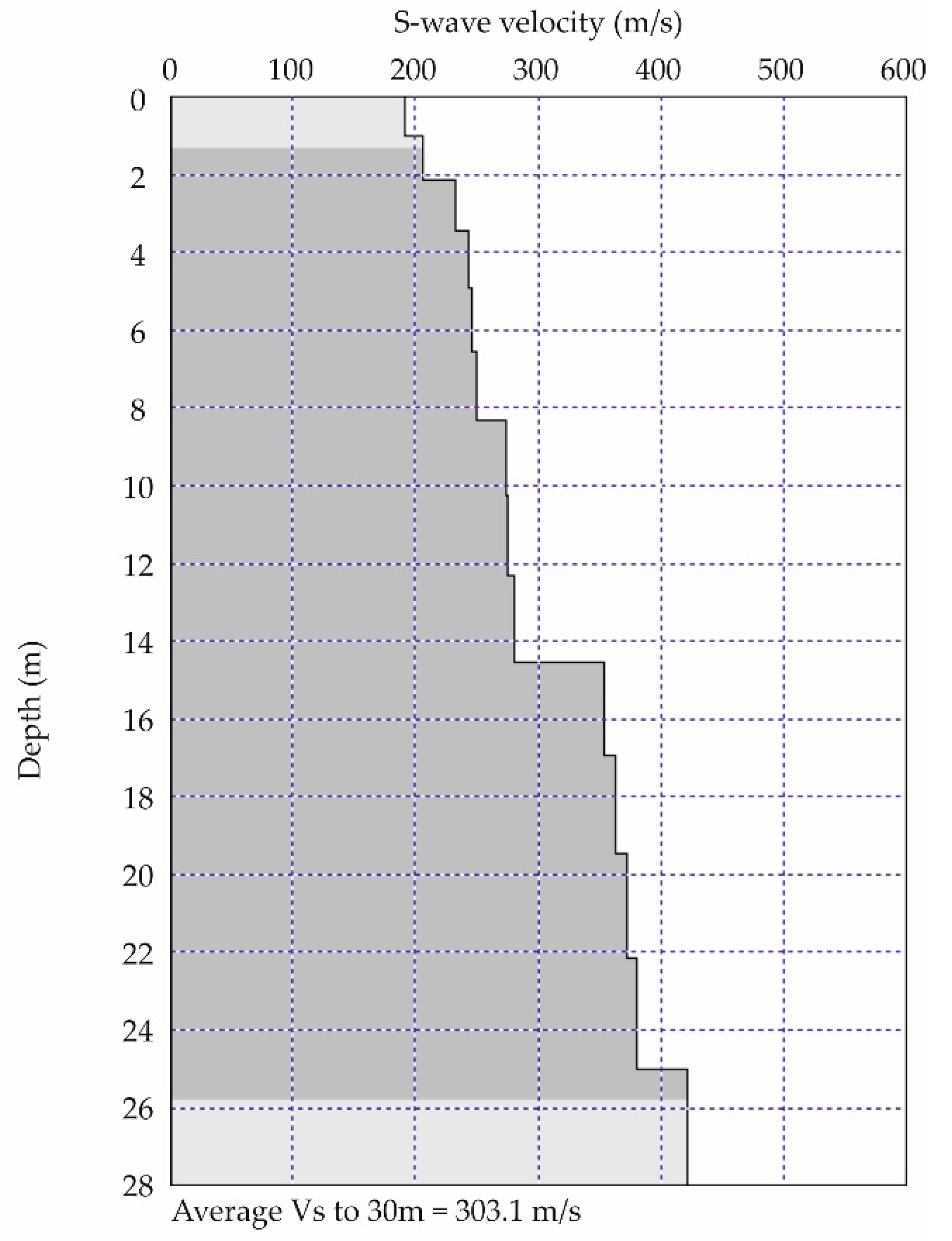
3.4. Seismological Station at Thalero, Korinthia (THAL)
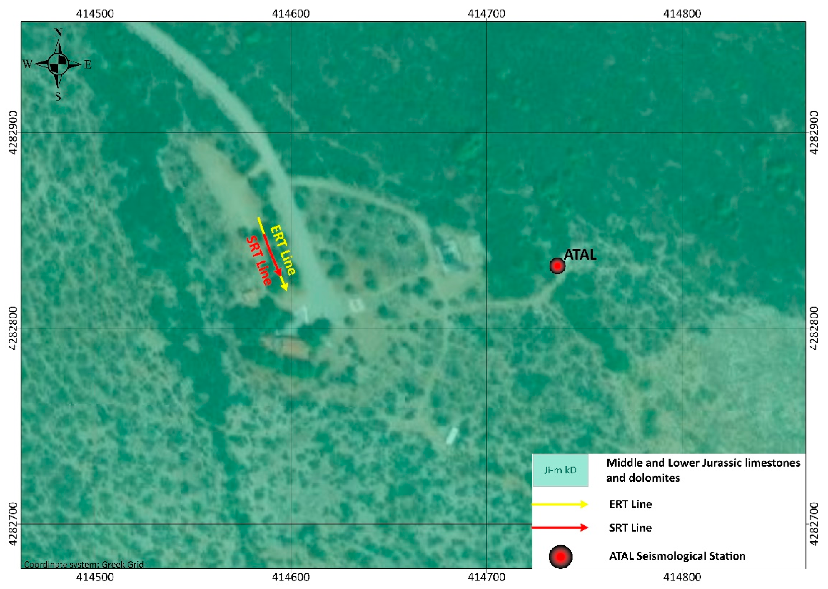
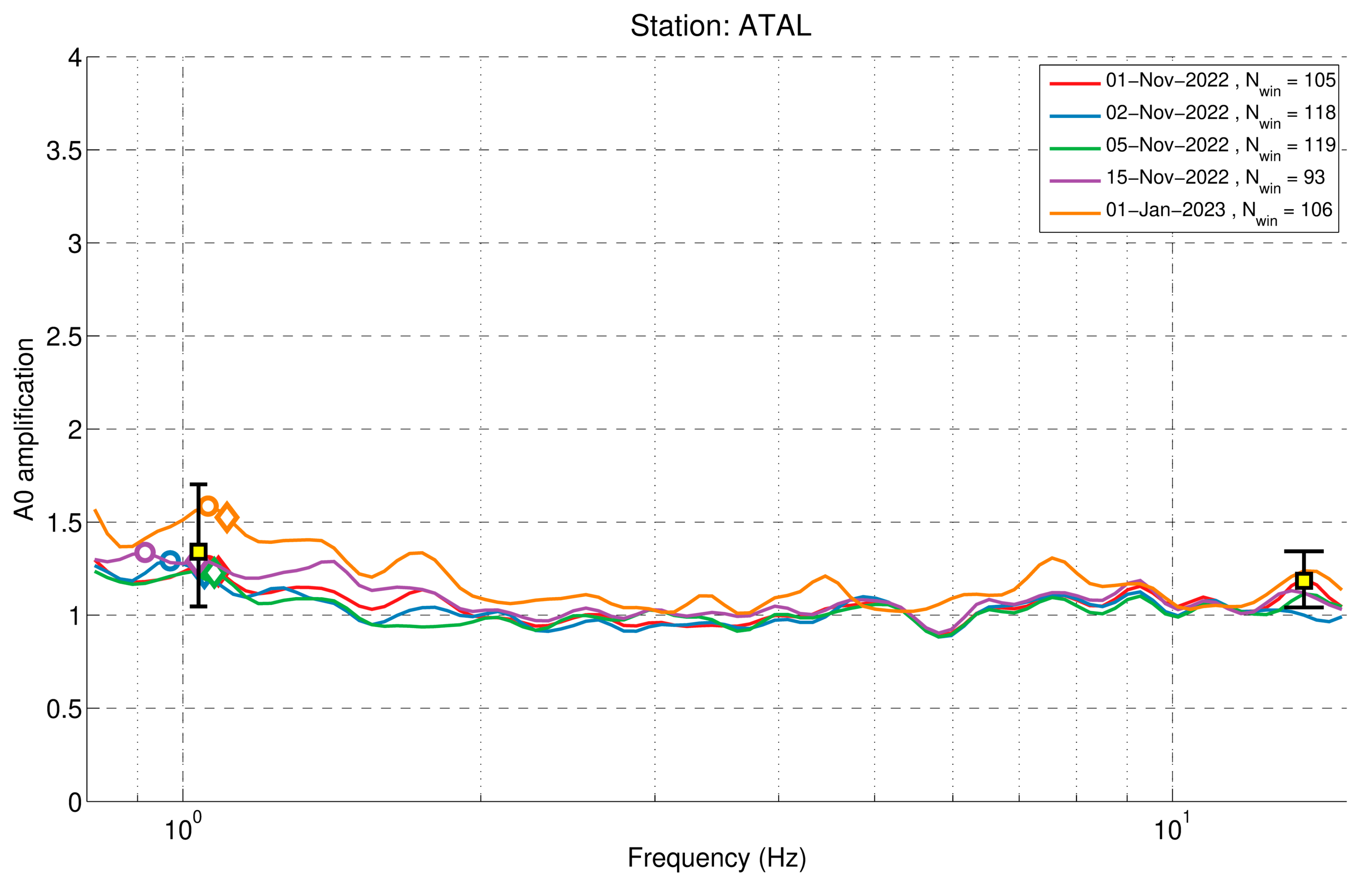
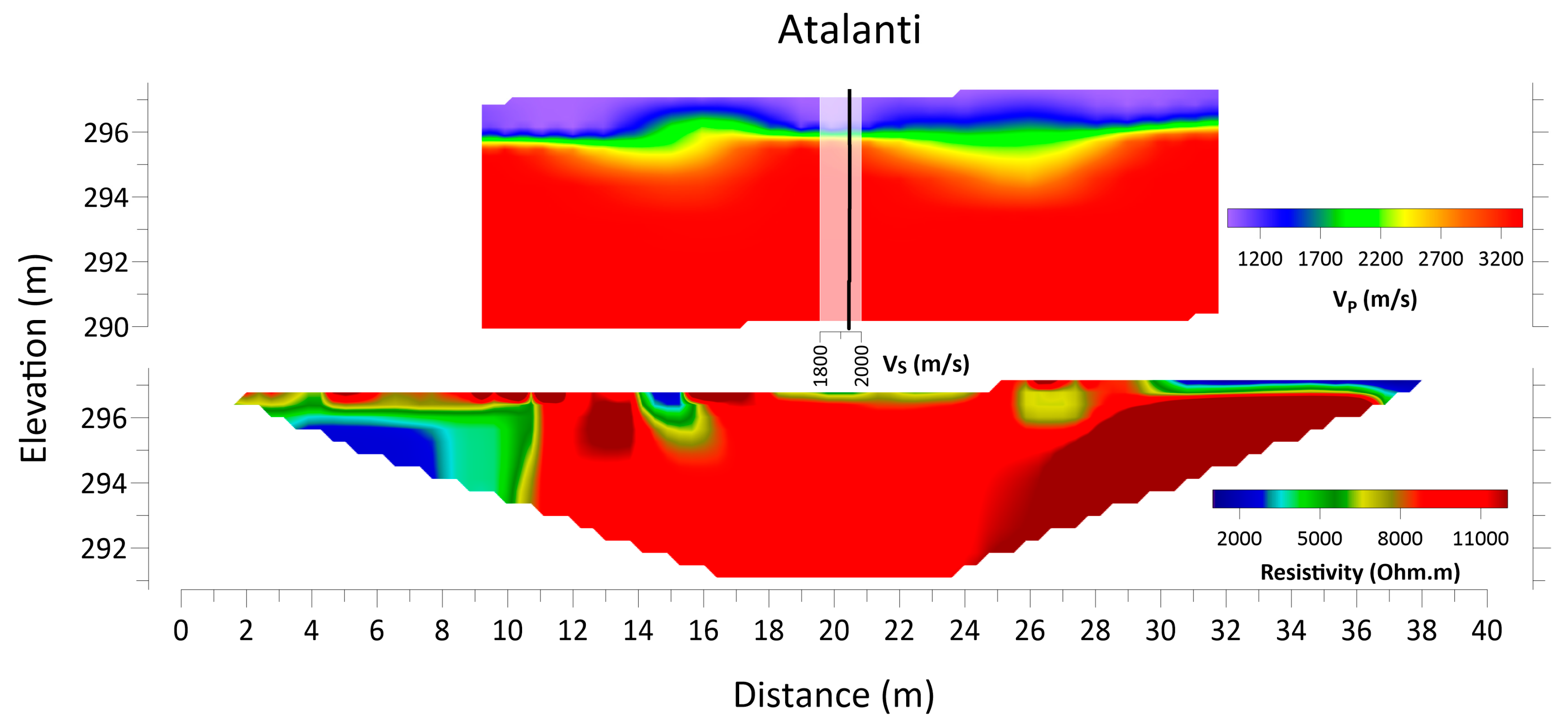
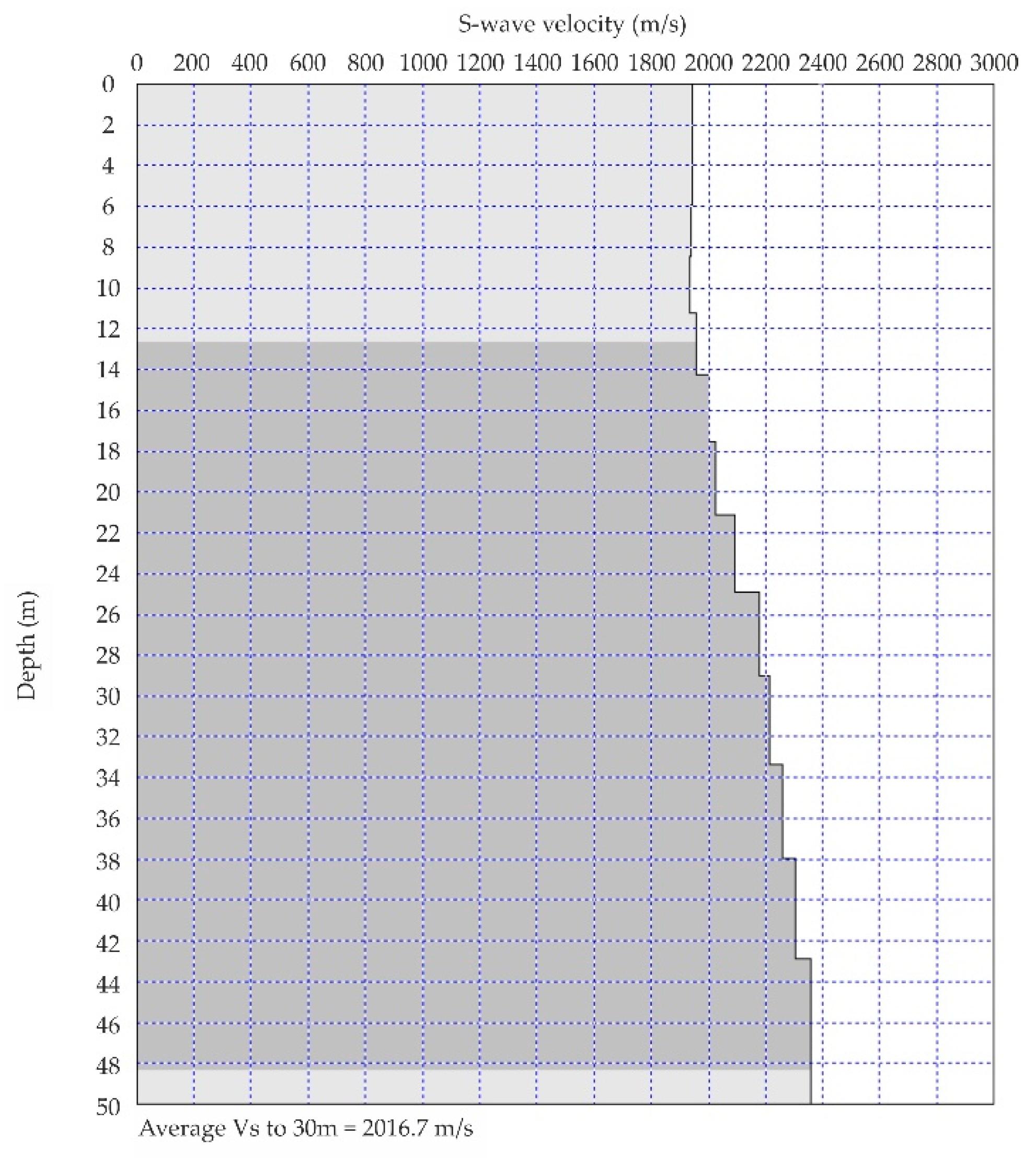
3.5. Seismological Station at Atalanti, Fthiotida (ATAL)
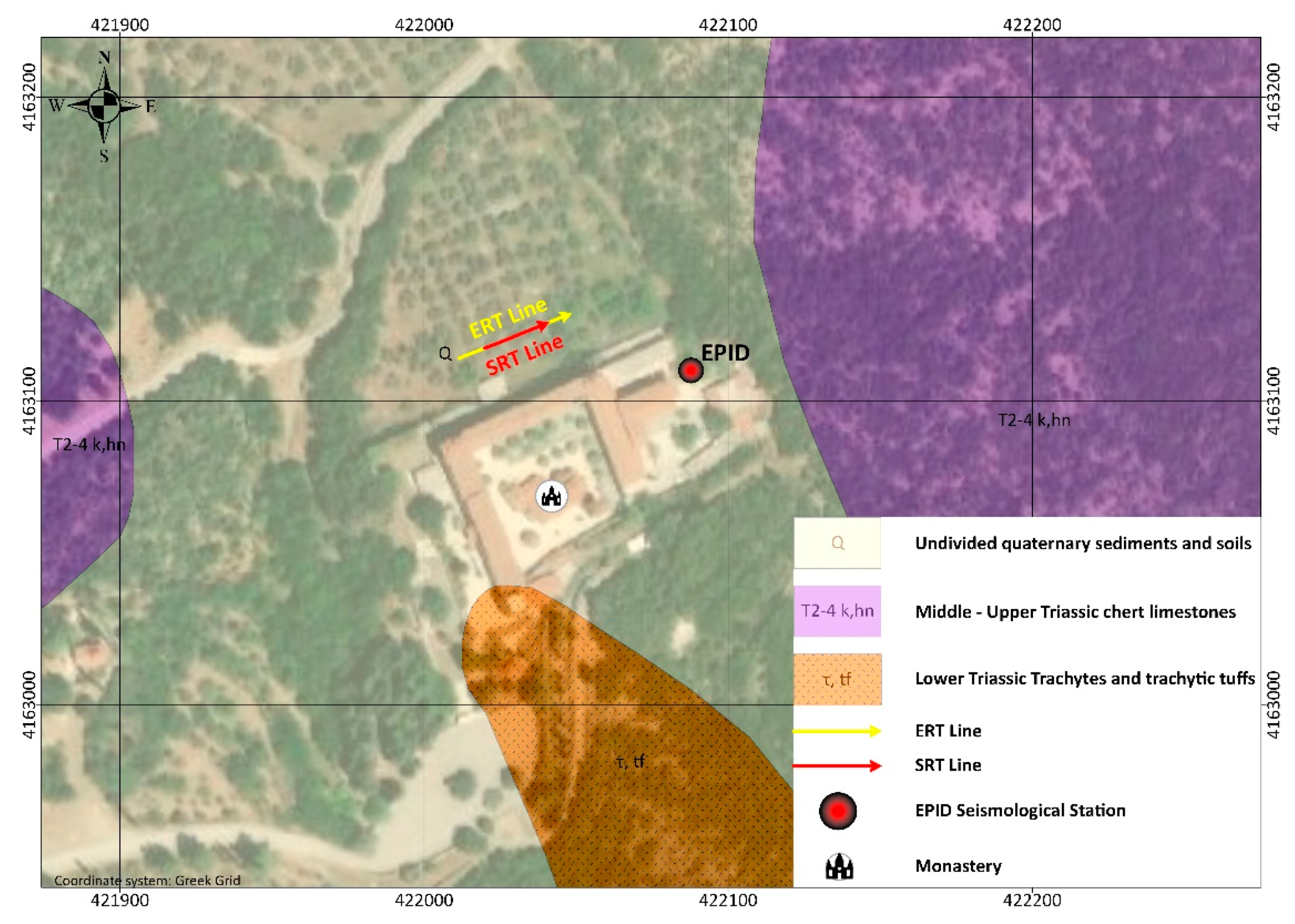
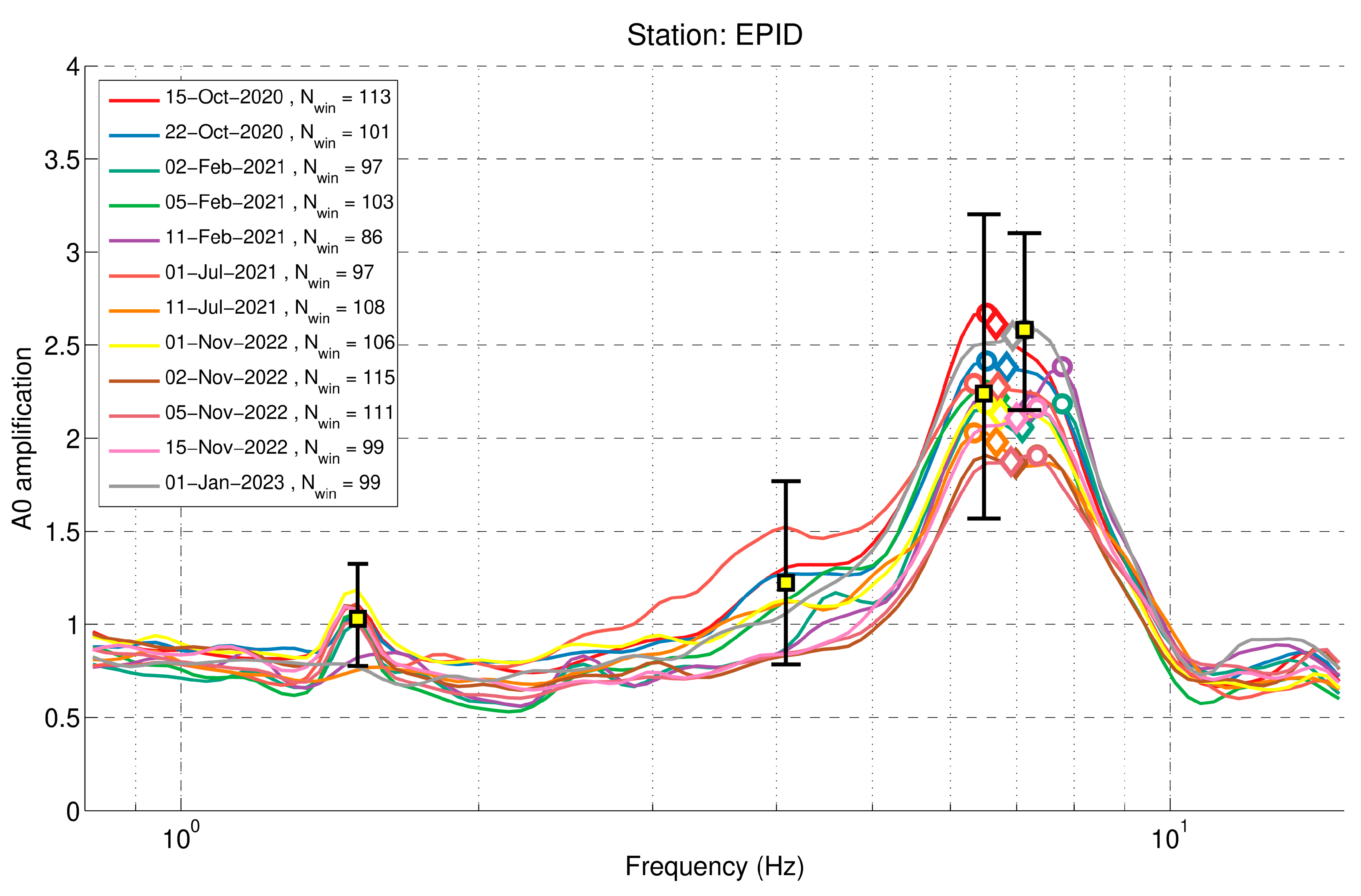
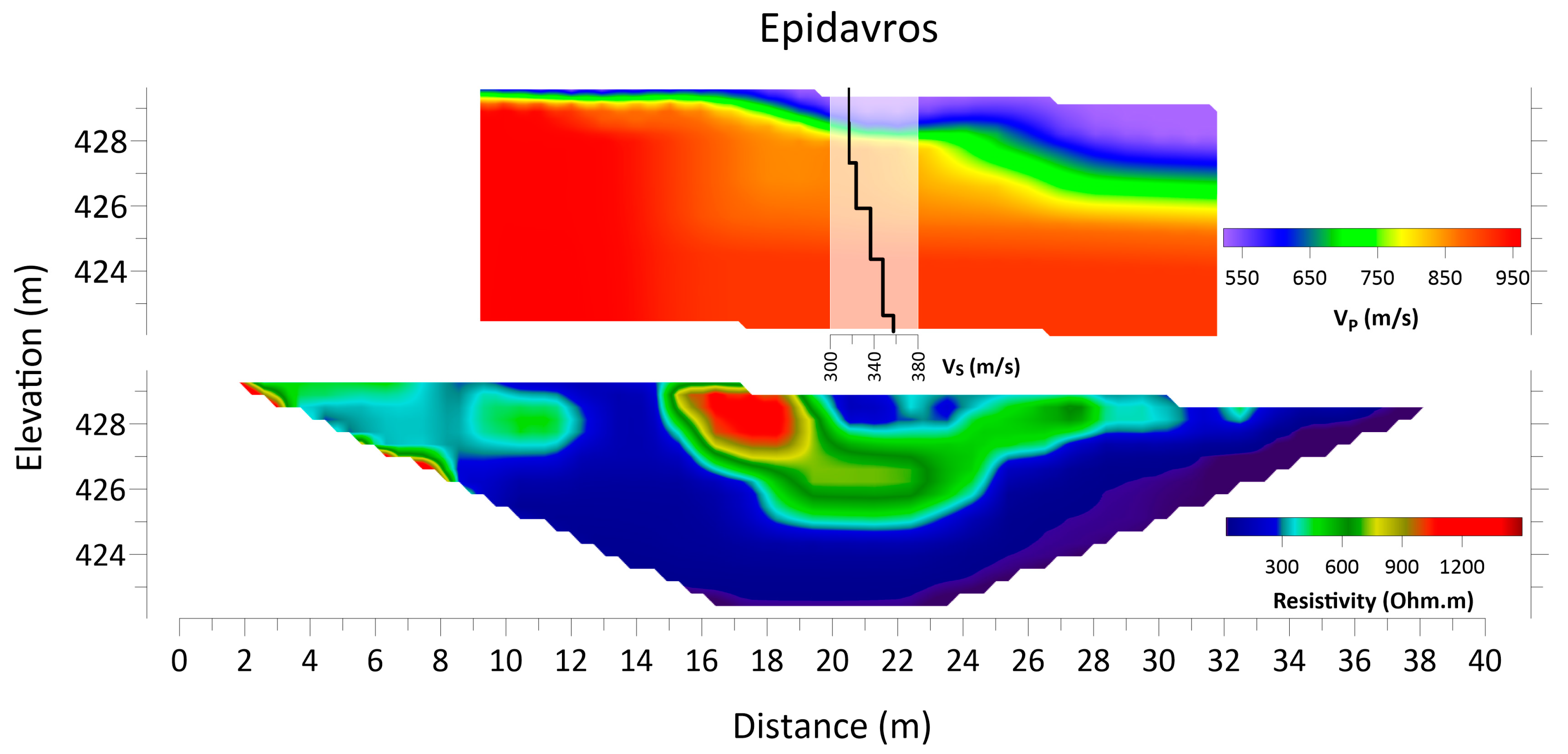
3.6. Seismological Station at Epidavros, Argolis (EPID)
4. Determination of Elastic Moduli
5. Results and Discussion
6. Conclusions
Author Contributions
Funding
Data Availability Statement
Acknowledgments
Conflicts of Interest
Appendix A

Appendix B


Appendix C

| f1 (Hz) | A1 | f2 (Hz) | A2 | f3 (Hz) | A3 | f4 (Hz) | A4 | |
|---|---|---|---|---|---|---|---|---|
| MDRA | 1.6 ± 0.1 | 1.4 ± 0.3 | 2.3 * | 1.7 ± 0.3 | 2.7 | 1.7 ± 0.3 | ||
| VILL | 1.2 | 1.8 ± 0.4 | 1.5 | 1.9 ± 0.4 | 10.4 * | 1.9 ± 0.3 | ||
| LOUT | 1.4 | 2.3 ± 0.5 | 2.5 ± 0. 1 | 2.6 ± 0.1 | 2.7 * | 3.1 ± 0.7 | 5.1 ± 0.1 | 2.2 ± 0.4 |
| THAL | 1.4 * | 1.7 ± 0.4 | 2.3 | 1.6 ± 0.3 | ||||
| ATAL | 1.0 * | 1.3 ± 0.3 | 13.6 | 1.2 ± 0.2 | ||||
| EPID | 1.5 ± 0.1 | 1.0 ± 0.3 | 4.1 ± 0.1 | 1.3 ± 0.5 | 6.5 ± 0.1 | 2.3 ± 0.8 | 7.1 * | 2.6 ± 0.5 |
References
- University of Athens. Hellenic Seismological Network, University of Athens, Seismological Laboratory [Data set]. International Federation of Digital Seismograph Networks. 2008. Available online: https://www.fdsn.org/networks/detail/HA/ (accessed on 20 March 2023).
- Evangelidis, C.P.; Triantafyllis, N.; Samios, M.; Boukouras, K.; Kontakos, K.; Ktenidou, O.-J.; Fountoulakis, I.; Kalogeras, I.; Melis, N.S.; Galanis, O.; et al. Seismic Waveform Data from Greece and Cyprus: Integration, Archival, and Open Access. Seismol. Res. Lett. 2021, 92, 1672–1684. Available online: https://pubs.geoscienceworld.org/ssa/srl/article-abstract/92/3/1672/595244/Seismic-Waveform-Data-from-Greece-and-Cyprus?redirectedFrom=fulltext (accessed on 20 March 2023). [CrossRef]
- National Observatory of Athens, Institute of Geodynamics, Athens. National Observatory of Athens Seismic Network [Data Set]. International Federation of Digital Seismograph Networks. 1975. Available online: https://www.fdsn.org/networks/detail/HL/ (accessed on 20 March 2023).
- Aristotle University of Thessaloniki. Aristotle University of Thessaloniki Seismological Network [Data Set]. International Federation of Digital Seismograph Networks. 1981. Available online: https://www.fdsn.org/networks/detail/HT/ (accessed on 20 March 2023).
- University of Patras. University of Patras, Seismological Laboratory [Data Set]. International Federation of Digital Seismograph Networks. 2000. Available online: https://www.fdsn.org/networks/detail/HP/ (accessed on 20 March 2023).
- Technological Educational Institute of Crete. Seismological Network of Crete [Data Set]. International Federation of Digital Seismograph Networks. 2006. Available online: https://www.fdsn.org/networks/detail/HC/ (accessed on 20 March 2023).
- Institute of Engineering Seimology Earthquake Engineering. ITSAK Strong Motion Network [Data Set]. International Federation of Digital Seismograph Networks. 1981. Available online: https://www.fdsn.org/networks/detail/HI/ (accessed on 20 March 2023).
- Rodriguez-Marek, A.; Rathje, E.M.; Bommer, J.J.; Scherbaum, F.; Stafford, P.J. Application of single-station sigma and site-response characterization in a probabilistic seismic-hazard analysis for a new nuclear site. Bull. Seismol. Soc. Am. 2014, 104, 1601–1619. [Google Scholar] [CrossRef] [Green Version]
- Bindi, D.; Cotton, F.; Kotha, S.R.; Bosse, C.; Stromeyer, D.; Grünthal, G. Application-driven ground motion prediction equation for seismic hazard assessments in non-cratonic moderate-seismicity areas. J. Seismol. 2017, 21, 1201–1218. [Google Scholar] [CrossRef] [Green Version]
- Bindi, D.; Parolai, S.; Gómez-Capera, A.; Locati, M.; Kalmetyeva, Z.; Mikhailova, N. Locations and magnitudes of earthquakes in Central Asia from seismic intensity data. J. Seismol. 2014, 18, 1–21. [Google Scholar] [CrossRef]
- Lanzano, G.; Luzi, L.; D’Amico, V.; Pacor, F.; Meletti, C.; Marzocchi, W.; Rotondi, R.; Varini, E. Ground motion models for the new seismic hazard model of Italy (MPS19): Selection for active shallow crustal regions and subduction zones. Bull. Earthq. Eng. 2020, 18, 3487–3516. [Google Scholar] [CrossRef]
- Priolo, E.; Pacor, F.; Spallarossa, D.; Milana, G.; Laurenzano, G.; Romano, M.A.; Felicetta, C.; Hailemikael, S.; Cara, F.; Di Giulio, G.; et al. Seismological analyses of the seismic microzonation of 138 municipalities damaged by the 2016–2017 seismic sequence in Central Italy. Bull. Earthq. Eng. 2020, 18, 5553–5593. [Google Scholar] [CrossRef] [Green Version]
- Al-Heety, A.J.; Hassouneh, M.; Abdullah, F.M. Application of MASW and ERT methods for geotechnical site characterization: A case study for roads construction and infrastructure assessment in Abu Dhabi, UAE. J. Appl. Geophys. 2021, 193, 104408. [Google Scholar] [CrossRef]
- Cardarelli, E.; Cercato, M.; De Donno, G. Characterization of an earth-filled dam through the combined use of electrical resistivity tomography, P-and SH-wave seismic tomography and surface wave data. J. Appl. Geophys. 2014, 106, 87–95. [Google Scholar] [CrossRef]
- Mohammed, M.A.; Abudeif, A.M.; Abd El-aal, A.K. Engineering geotechnical evaluation of soil for foundation purposes using shallow seismic refraction and MASW in 15th Mayo, Egypt. J. Afr. Earth Sci. 2020, 162, 103721. [Google Scholar] [CrossRef]
- Pegah, E.; Liu, H. Application of near-surface seismic refraction tomography and multichannel analysis of surface waves for geotechnical site characterizations: A case study. Eng. Geol. 2016, 208, 100–113. [Google Scholar] [CrossRef]
- Romero-Ruiz, A.; Linde, N.; Keller, T.; Or, D. A review of geophysical methods for soil structure characterization. Rev. Geophys. 2018, 56, 672–697. [Google Scholar] [CrossRef] [Green Version]
- Salem, H.S. Poisson’s ratio and the porosity of surface soils and shallow sediments, determined from seismic compressional and shear wave velocities. Geotechnique 2000, 50, 461–463. [Google Scholar] [CrossRef]
- Cultrera, G.; Cornou, C.; Di Giulio, G.; Bard, P.Y. Indicators for site characterization at seismic station: Recommendation from a dedicated survey. Bull. Earthq. Eng. 2021, 19, 4171–4195. [Google Scholar] [CrossRef]
- Macau, A.; Benjumea, B.; Gabàs, A.; Figueras, S. Optimal Application of Geophysical Techniques for Subsoil Characterization of Seismic Stations. In Proceedings of the Near Surface Geoscience 2015-21st European Meeting of Environmental and Engineering Geophysics, Turin, Italy, 6–10 September 2015; European Association of Geoscientists & Engineers: Utrecht, The Netherlands, 2015; Volume 1, pp. 1–5. [Google Scholar] [CrossRef]
- Leyton, F.; Leopold, A.; Hurtado, G.; Pastén, C.; Ruiz, S.; Montalva, G.; Saéz, E. Geophysical characterization of the Chilean seismological stations: First results. Seismol. Res. Lett. 2018, 89, 519–525. [Google Scholar] [CrossRef] [Green Version]
- Di Giulio, G.; Cultrera, G.; Cornou, C.; Bard, P.Y.; Al Tfaily, B. Quality assessment for site characterization at seismic stations. Bull. Earthq. Eng. 2021, 19, 4643–4691. [Google Scholar] [CrossRef]
- Farrugia, J.J.; Molnar, S.; Atkinson, G.M. Noninvasive Techniques for Site Characterization of Alberta Seismic Stations Based on Shear-Wave Velocity. Bull. Seismol. Soc. Am. 2017, 107, 2885–2902. [Google Scholar] [CrossRef]
- Nakamura, Y. A method for dynamic characteristics estimation of subsurface using microtremor on the ground surface. Railw. Tech. Res. Inst. Q. Rep. 1989, 30, 25–33. [Google Scholar]
- Gorstein, M.; Ezersky, M. Combination of HVSR and MASW Methods to Obtain Shear Wave Velocity Model of Subsurface in Israel. Int. J. Georesources Environ. -IJGE 2015, 1, 20–41. [Google Scholar] [CrossRef]
- Stanko, D.; Markušić, S.; Strelec, S.; Gazdek, M. HVSR Analysis of Seismic Site Effects and Soil-Structure Resonance in Varaždin City (North Croatia). Soil Dyn. Earthq. Eng. 2017, 92, 666–677. [Google Scholar] [CrossRef]
- Fat-Helbary, R.E.-S.; El-Faragawy, K.O.; Hamed, A. Application of HVSR Technique in the Site Effects Estimation at the South of Marsa Alam City, Egypt. J. Afr. Earth Sci. 2019, 154, 89–100. [Google Scholar] [CrossRef]
- Arimuko, A.; Santoso, E.; Sunardi, B. Investigation of Site Condition Using Elliptical Curve Inversion from Horizontal-to-Vertical Spectral Ratio (HVSR). J. Phys. Conf. Ser. 2020, 1491, 012031. [Google Scholar] [CrossRef]
- Capizzi, P.; Martorana, R. Analysis of HVSR Data Using a Modified Centroid-Based Algorithm for Near-Surface Geological Reconstruction. Geosciences 2022, 12, 147. [Google Scholar] [CrossRef]
- Napolitano, F.; Gervasi, A.; La Rocca, M.; Guerra, I.; Scarpa, R. Site effects in the pollino region from the HVSR and polarization of seismic noise and earthquakes site effects in the pollino region from the HVSR and polarization of seismic noise and earthquakes. Bull. Seismol. Soc. Am. 2018, 108, 309–321. [Google Scholar] [CrossRef]
- La Rocca, M.; Chiappetta, G.D.; Gervasi, A.; Festa, R.L. Non-stability of the noise HVSR at sites near or on topographic heights. Geophys. J. Int. 2020, 222, 2162–2171. [Google Scholar] [CrossRef]
- Kassaras, I.; Kalantoni, D.; Kouskouna, V.; Pomonis, A.; Michalaki, K.; Stoumpos, P.; Mourloukos, S.; Birmpilopoulos, S.; Makropoulos, K. Correlation between damage distribution and soil characteristics deduced from ambient vibrations in the old town of Lefkada (W Greece). In Proceedings of the 2nd European Conference on Earthquake Engineering and Seismology, Istanbul, Turkey, 25–29 August 2014. Paper n. 251. [Google Scholar]
- Kassaras, I.; Papadimitriou, P.; Kapetanidis, V.; Voulgaris, N. Seismic Site Characterization at the Western Cephalonia Island in the Aftermath of the 2014 Earthquake Series. Int. J. Geo-Eng. 2017, 8, 1–22. [Google Scholar] [CrossRef] [Green Version]
- Kassaras, I.; Kazantzidou-Firtinidou, D.; Ganas, A.; Kapetanidis, V.; Tsimi, C.; Valkaniotis, S.; Sakellariou, N.; Mourloukos, S. Seismic Risk and Loss Assessment for Kalamata (SW Peloponnese, Greece) from Neighbouring Shallow Sources. Boll. Di Geofis. Teor. Ed Appl. 2018, 59, 1–26. [Google Scholar] [CrossRef]
- Theodoulidis, N.; Cultrera, G.; Cornou, C.; Bard, P.-Y.; Boxberger, T.; DiGiulio, G.; Imtiaz, A.; Kementzetzidou, D.; Makra, K.; The Argostoli NERA Team. Basin Effects on Ground Motion: The Case of a High-Resolution Experiment in Cephalonia (Greece). Bull. Earthq. Eng. 2018, 16, 529–560. [Google Scholar] [CrossRef]
- Rigo, A.; Sokos, E.; Lefils, V.; Briole, P. Seasonal Variations in Amplitudes and Resonance Frequencies of the HVSR Amplification Peaks Linked to Groundwater. Geophys. J. Int. 2021, 226, 1–13. [Google Scholar] [CrossRef]
- Adewoyin, O.O.; Joshua, E.O.; Akinyemi, M.L.; Omeje, M.; Adagunodo, T.A. Evaluation of geotechnical parameters of reclaimed land from near-surface seismic refraction method. Heliyon 2021, 7, e06765. [Google Scholar] [CrossRef]
- Khalil, M.H.; Hanafy, S.M. Engineering applications of seismic refraction method: A field example at Wadi Wardan, Northeast Gulf of Suez, Sinai, Egypt. J. Appl. Geophys. 2008, 65, 132–141. [Google Scholar] [CrossRef]
- Yilmaz, O.; Eser, M.; Berilgen, M. Seismic, geotechnical, and earthquake engineering site characterization. In SEG Technical Program Expanded Abstracts; Society of Exploration Geophysicists: Tulsa, OK, USA, 2006; pp. 1401–1405. [Google Scholar] [CrossRef] [Green Version]
- Zhang, J.; Toksöz, M.N. Nonlinear refraction traveltime tomography. Geophysics 1998, 63, 1726–1737. [Google Scholar] [CrossRef]
- Zhu, X.; Sixta, D.P.; Angstman, B.G. Tomostatics: Turning-ray tomography+ static corrections. Lead. Edge 1992, 11, 15–23. [Google Scholar] [CrossRef]
- Stefani, J.P. Turning-ray tomography. Geophysics 1995, 60, 1917–1929. [Google Scholar] [CrossRef]
- Lanz, E.; Maurer, H.; Green, A.G. Refraction tomography over a buried waste disposal site. Geophysics 1998, 63, 1414–1433. [Google Scholar] [CrossRef]
- Thurber, C.; Ritsema, J. Theory and observations-seismic tomography and inverse methods. Seismol. Struct. Earth 2007, 1, 323–360. [Google Scholar] [CrossRef]
- Foti, S.; Parolai, S.; Albarello, D.; Picozzi, M. Application of surface-wave methods for seismic site characterization. Surv. Geophys. 2011, 32, 777–825. [Google Scholar] [CrossRef] [Green Version]
- Socco, L.V.; Strobbia, C. Surface-wave method for near-surface characterization: A tutorial. Near Surf. Geophys. 2004, 2, 165–185. [Google Scholar] [CrossRef]
- Park, C.B.; Miller, R.D.; Xia, J. Multichannel analysis of surface waves. Geophysics 1999, 64, 800–808. [Google Scholar] [CrossRef] [Green Version]
- Eker, A.M.; Akgün, H.; Koçkar, M.K. Local site characterization and seismic zonation study by utilizing active and passive surface wave methods: A case study for the northern side of Ankara, Turkey. Eng. Geol. 2012, 151, 64–81. [Google Scholar] [CrossRef]
- Kanlı, A.I.; Tildy, P.; Prónay, Z.; Pınar, A.; Hermann, L. VS30 mapping and soil classification for seismic site effect evaluation in Dinar region, SW Turkey. Geophys. J. Int. 2006, 165, 223–235. [Google Scholar] [CrossRef] [Green Version]
- Karabulut, S. Soil classification for seismic site effect using MASW and ReMi methods: A case study from western Anatolia (Dikili-İzmir). J. Appl. Geophys. 2018, 150, 254–266. [Google Scholar] [CrossRef]
- Xia, J.; Miller, R.D.; Park, C.B.; Hunter, J.A.; Harris, J.B.; Ivanov, J. Comparing shear-wave velocity profiles inverted from multichannel surface wave with borehole measurements. Soil Dyn. Earthq. Eng. 2002, 22, 181–190. [Google Scholar] [CrossRef]
- SESAME. Guidelines for Implementation of the H/V Spectral Ratio Technique on AMBIENT Vibrations: Measurements, Processing and Interpretation, European Commission–EVG1-CT-2000-00026 SESAME. 2004. Available online: http://sesame.geopsy.org/Papers/HV_User_Guidelines.pdf (accessed on 9 March 2023).
- Allen, R.V. Automatic Earthquake Recognition and Timing from Single Traces. Bull. Seismol. Soc. Am. 1978, 68, 1521–1532. [Google Scholar] [CrossRef]
- Konno, K.; Ohmachi, T. Ground-Motion Characteristics Estimated from Spectral Ratio between Horizontal and Vertical Components of Microtremor. Bull. Seismol. Soc. Am. 1998, 88, 228–241. [Google Scholar] [CrossRef]
- Geometrics Inc.; OYO Inc. SeisImager Manual Version 3.3 [Computer Program Manual]; OYO Corporation: Tokyo, Japan, 2009. [Google Scholar]
- Babuska, V.; Cara, M. Seismic Anisotropy in the Earth; Kluwer Academic Publishers: Boston, MA, USA, 1991. [Google Scholar]
- EN 1998-1; Eurocode 8: Design of Structures for Earthquake Resistance. Part 1: General Rules, Seismic Actions and Rules for Buildings. European Committee for Standardization (CEN): Brussels, Belgium, 2004.
- Alexopoulos, J.D.; Voulgaris, N.; Dilalos, S.; Gkosios, V.; Giannopoulos, I.K.; Mitsika, G.S.; Vassilakis, E.m.; Sakkas, V.; Kaviris, G. Near-Surface Geophysical Characterization of Lithologies in Corfu and Lefkada Towns (Ionian Islands, Greece). Geosciences 2022, 12, 446. [Google Scholar] [CrossRef]
- Vasilatos, C.; Anastasatou, M.; Alexopoulos, J.; Vassilakis, E.; Dilalos, S.; Antonopoulou, S.; Petrakis, S.; Delipetrou, P.; Georghiou, K.; Stamatakis, M. Assessment of the Geo-Environmental Status of European Union Priority Habitat Type “Mediterranean Temporary Ponds” in Mt. Oiti, Greece. Water 2019, 11, 1627. [Google Scholar] [CrossRef] [Green Version]
- Alexopoulos, J.D.; Dilalos, S.; Vassilakis, E. Adumbration of Amvrakia’s spring water pathways, based on detailed geophysical data (Kastraki-Meteora). Adv. Res. Aquat. Environ. 2011, 2, 105–112. [Google Scholar] [CrossRef]
- Abzalov, M.Z. Measuring and modelling of dry bulk rock density for mineral resource estimation. Appl. Earth Sci. 2013, 122, 16–29. [Google Scholar] [CrossRef]
- Dilalos, S. Application of Geophysical Technique to the Investigation of Tectonic Structures in Urban and Suburban Environments. A Case Study in Athens Basin. Ph.D. Thesis, National and Kapodistrian University of Athens, Athens, Greece, 2018. Available online: http://hdl.handle.net/10442/hedi/48791 (accessed on 20 March 2023).
- Dilalos, S.; Alexopoulos, J.D.; Lozios, S. New insights on Athens basin (Greece) subsurface geological and tectonic structure, derived from urban gravity measurements. J. Appl. Geophys. 2019, 167, 73–105. [Google Scholar] [CrossRef]
- Dilalos, S.; Alexopoulos, J.D.; Vassilakis, E.; Poulos, S.E. Investigation of the structural control of a deltaic valley with geophysical methods. The case study of Pineios river delta (Thessaly, Greece). J. Appl. Geophys. 2022, 202, 104652. [Google Scholar] [CrossRef]
- García-Pérez, T.; Marquardt, C.; Yáñez, G.; Cembrano, J.; Gomila, R.; Santibañez, I.; Maringue, J. Insights on the structural control of a Neogene forearc basin in Northern Chile: A geophysical approach. Tectonophysics 2018, 736, 1–14. [Google Scholar] [CrossRef]
- Parasnis, D.S. A study of rock densities in the English Midlands. Geophys. Suppl. Mon. Not. R. Astron. Soc. 1952, 6, 252–271. [Google Scholar] [CrossRef] [Green Version]
- Lee, C.S.; Cho, T.C.; Lee, S.B.; Won, K.S. A study of weathering characteristic of Baeknokdam trachyte in Jeju Island. J. Eng. Geol. 2007, 17, 235–251. [Google Scholar]
- Dounas, A. Geological Map of Greece, Sheet Erythrai, Scale 1:50.000; Institute of Geological and Mineralogical of Greece: Athens, Greece, 1971. [Google Scholar]
- Papadimitriou, P.; Kaviris, G.; Makropoulos, K. Evidence of shear wave splitting in the eastern Korinthian Gulf (Greece). Phys. Earth Planet. Inter. 1999, 114, 3–13. [Google Scholar] [CrossRef]
- Kaviris, G. Study of Seismic Source Properties of the Eastern Gulf of Corinth. Ph.D. Thesis, Faculty of Geology, University of Athens, Athens, Greece, 2003. [Google Scholar]
- Bornovas, J.; Lalechos, N.; Filippakis, N. Geological Map of Greece, Sheet Korinthos, Scale 1:50.000; Institute of Geological and Mineralogical of Greece: Athens, Greece, 1969. [Google Scholar]
- Koutsouveli, A.; Mettos, A. Geological Map of Greece, Sheet Xilokastron, Scale 1:50.000; Institute of Geological and Mineralogical of Greece: Athens, Greece, 1983. [Google Scholar]
- Maratos, G. Geological Map of Greece, Sheet Atalanti, Scale 1:50.000; Institute of Geological and Mineralogical of Greece: Athens, Greece, 1965. [Google Scholar]
- Bannert, D. Geological Map of Greece, Sheet Ligourion, Scale 1:50.000; Institute of Geological and Mineralogical of Greece: Athens, Greece, 1972. [Google Scholar]
- Basheer, A.A.; Salama, N.S. Application of ERT and SSR for geotechnical site characterization: A case study for resort assessment in New El Alamein City, Egypt. NRIAG J. Astron. Geophys. 2022, 11, 58–68. [Google Scholar] [CrossRef]
- Fat-Helbary, R.E.S.; El-Faragawy, K.O.; Hamed, A. Soil geotechnical characteristics for seismic risk mitigation at the southern extension of Marsa Alam city, Egypt. NRIAG J. Astron. Geophys 2019, 8, 1–14. [Google Scholar] [CrossRef] [Green Version]
- Gkosios, V.; Alexopoulos, J.D.; Giannopoulos, I.K.; Mitsika, G.S.; Dilalos, S.; Barbaresos, I.; Voulgaris, N. Determination of the subsurface geological regime and geotechnical characteristics at the area of Goudi (Athens, Greece) derived from geophysical measurements. Bulletin of the Geological Society of Greece, Special Publication GSG2022-062. In Proceedings of the 16th International Congress of the Geological Society of Greece, Patras, Greece, 17–19 October 2022. [Google Scholar]
- Giannopoulos, I.K.; Alexopoulos, J.D.; Dilalos, S.; Gkosios, V.; Mitsika, G.S.; Stamatakis, M.; Voulgaris, N. The geophysical identification of lateritic bauxite formation at Mandra area, Attiki (Greece). Bulletin of the Geological Society of Greece, Special Publication No 10, GSG2022-026. In Proceedings of the 16th International Congress of the Geological Society of Greece, Patras, Greece, 17–19 October 2022. [Google Scholar]
- Mitsika, G.S.; Alexopoulos, J.D.; Giannopoulos, I.K.; Gkosios, V.; Dilalos, S.; Filis, C.; Vassilakis, E.m.; Kaviris, G.; Sakkas, V.; Voulgaris, N. Preliminary results of near-surface geophysical survey in Lefkada town (Greece). Bulletin of the Geological Society of Greece, Special Publication No 10, GSG2022-031. In Proceedings of the 16th International Congress of the Geological Society of Greece, Patras, Greece, 17–19 October 2022. [Google Scholar]
- Adams, L.H. Elastic Properties of Materials of the Earth’s Crust. In Internal Construction of the Earth (Edited by Gutenberg); Dover Publications, Inc.: New York, NY, USA, 1951. [Google Scholar]
- Toksöz, M.N.; Cheng, C.H.; Timur, A. Velocities of seismic waves in porous rocks. Geophysics 1976, 41, 621–645. [Google Scholar] [CrossRef]
- Ibs-von Seht, M.; Wohlenberg, J. Microtremors measurement used to map thickness of soft soils sediments. Bull. Seismol. Soc. Am. 1999, 89, 250–259. [Google Scholar] [CrossRef]


| Ground Type | Description of Stratigraphic Profile | |
|---|---|---|
| A | Rock or other rock-like geological formations, including at most 5 m of weaker material at the surface. | >800 |
| B | Deposits of very dense sand, gravel, or very stiff clay, at least several tens of meters in thickness, characterized by a gradual increase of mechanical properties with depth. | 360–800 |
| C | Deep deposits of dense or medium-dense sand, gravel, or stiff clay with thickness from several tens to many hundreds of meters. | 180–360 |
| D | Deposits of loose-to-medium cohesionless soil (with or without some soft cohesive layers), or of predominantly soft-to-firm cohesive soil. | <180 |
| Seismological Station | Geological Formation | Number of Specimens | Dry Density (gr/cm3) | Saturated Density (gr/cm3) | Standard Deviation |
|---|---|---|---|---|---|
| MDRA | Dolostones, dolomitic limestones, and limestones (TRm) | 20 | 2.69 | 2.69 | 0.02 |
| VILL | Dolostones, dolomitic limestones, and limestones (TRm) | 20 | 2.66 | 2.67 | 0.03 |
| LOUT | Talus and scree cones | - | 2.3 * [62,63] | - | 0.10 |
| THAL | Marine-brackish marls (Pl-Pt.m) | - | 1.72 * [62,63] | - | 0.07 |
| ATAL | Limestones and dolomites (Ji-m kD) | 20 | 2.81 | 2.82 | 0.01 |
| EPID | Trachytes and trachytic tuffs (τ, tf) | - | 2.04 * [67] | - | - |
| Elastic Modulus | Equation | Reference |
|---|---|---|
| Poisson’s ratio (σ) | [80] | |
| Young’s modulus (E) | [80] | |
| Shear modulus (G) | [81] | |
| Bulk modulus (K) | [81] |
| Station Name | Geological Formations | VP (m/s) | VS (m/s) | Density (gr/cm3) | σ | G (GPa) | Ε (GPa) | K (GPa) | ρ (Ohm.m) |
|---|---|---|---|---|---|---|---|---|---|
| MDRA | Dolostones (TRm) | 3300 | 1860 | 2.69 | 0.27 | 9.31 | 23.59 | 22.31 | 9000 |
| VILL | Dolostones (TRm) | 2100 | 1160 | 2.66 | 0.28 | 3.58 | 9.17 | 9.05 | 8000 |
| LOUT | Talus cones (Q.cn) | 1330 | 500 | 2.30 [62,63] | 0.42 | 0.58 | 1.63 | 3.64 | 100 |
| THAL | Μarls (Pl-Pt.m) | 1600 | 250 | 1.72 [62,63] | 0.49 | 0.11 | 0.32 | 4.32 | 50 |
| ATAL | Limestones (Ji-m kD) | 3300 | 1940 | 2.81 | 0.24 | 10.58 | 26.14 | 22.67 | 9000 |
| EPID | Trachytes and trachytic tuffs (τ, tf) | 950 | 350 | 2.04 [67] | 0.42 | 0.25 | 0.71 | 1.65 | 250 |
| Station Name | Fundamental Frequency, f0 (Hz) | Seismic Bedrock Depth, Hseis (m) | VS (m/s) | VS30 (m/s) | Soil Type (EC8) [58] | Subsurface Geology |
|---|---|---|---|---|---|---|
| MDRA | - | - | 1830–2500 | 1877 | A | Dolostones, dolomitic limestones, and limestones |
| VILL | 10.4 | 13.0 | 1160–1500 | 1217 | A | Dolostones, dolomitic limestones, and limestones |
| LOUT | 2.7 | 30.0 | 300–900 | 638 | B | Old talus cones and scree formation, shales–chert, and limestone formations |
| THAL | 1.4 | 54.0 | 200–420 | 300 | C | Marine-brackish marls and conglomerates |
| ATAL | - | - | 1930–2350 | 2016 | A | Limestones and dolomites |
| EPID | 7.1 | 12.0 | 320–460 | 393 | B | Quaternary sediments, trachytes/trachytic tuffs, and chert limestones |
Disclaimer/Publisher’s Note: The statements, opinions and data contained in all publications are solely those of the individual author(s) and contributor(s) and not of MDPI and/or the editor(s). MDPI and/or the editor(s) disclaim responsibility for any injury to people or property resulting from any ideas, methods, instructions or products referred to in the content. |
© 2023 by the authors. Licensee MDPI, Basel, Switzerland. This article is an open access article distributed under the terms and conditions of the Creative Commons Attribution (CC BY) license (https://creativecommons.org/licenses/by/4.0/).
Share and Cite
Alexopoulos, J.D.; Dilalos, S.; Voulgaris, N.; Gkosios, V.; Giannopoulos, I.-K.; Kapetanidis, V.; Kaviris, G. The Contribution of Near-Surface Geophysics for the Site Characterization of Seismological Stations. Appl. Sci. 2023, 13, 4932. https://doi.org/10.3390/app13084932
Alexopoulos JD, Dilalos S, Voulgaris N, Gkosios V, Giannopoulos I-K, Kapetanidis V, Kaviris G. The Contribution of Near-Surface Geophysics for the Site Characterization of Seismological Stations. Applied Sciences. 2023; 13(8):4932. https://doi.org/10.3390/app13084932
Chicago/Turabian StyleAlexopoulos, John D., Spyridon Dilalos, Nicholas Voulgaris, Vasileios Gkosios, Ioannis-Konstantinos Giannopoulos, Vasilis Kapetanidis, and George Kaviris. 2023. "The Contribution of Near-Surface Geophysics for the Site Characterization of Seismological Stations" Applied Sciences 13, no. 8: 4932. https://doi.org/10.3390/app13084932