Article

The Importance of Soil Elevation and Hydroperiods in Salt Marsh Vegetation Zonation: A Case Study of Ria de Aveiro

by
Marisa Marques Gouveia
1,
Natasha Nonemacher Magni
1,
Carina Lurdes Lopes
2,*,
Américo Soares Ribeiro
2,
João Miguel Dias
2 and
Helena Silva
1
1
Centre for Environmental and Marine Studies (CESAM), Department of Biology, University of Aveiro, Campus de Santiago, 3810-193 Aveiro, Portugal
2
Centre for Environmental and Marine Studies (CESAM), Physics Department, University of Aveiro, Campus de Santiago, 3810-193 Aveiro, Portugal
*
Author to whom correspondence should be addressed.
Appl. Sci. 2023, 13(7), 4605; https://doi.org/10.3390/app13074605
Submission received: 23 February 2023 / Revised: 1 April 2023 / Accepted: 4 April 2023 / Published: 5 April 2023
(This article belongs to the Special Issue Recent Advances in Halophytes Plants)

Abstract

:
Salt marshes are among the most valuable ecosystems on earth; however, previous research has reported global losses in their extent accompanied by an impairment of their ecological processes. Nonetheless, investigations on salt marsh vegetation ecology are still lacking in many sites, including in Ria de Aveiro. As such, this study aimed to (1) monitor, characterize, and understand the evolution of salt marsh vegetation communities at three different study sites with different environmental conditions and stages of degradation, where we also sought to (2) identify the main delimiting abiotic factors associated with the distribution of the main species. To do so, a multidisciplinary approach that involved the survey of vegetation from permanent transects and the collection of ecological, physicochemical, and hydrodynamic data at sampling points within the monospecific stands of the main species was reported. The results showed that, of the abiotic factors deemed as the main delimiting forces of salt marsh vegetation, the soil elevation and hydroperiod were the most restrictive factors, as they ultimately influenced species composition at the different study sites and explained most of the variation observed between the studied monospecific stands.

1. Introduction

Salt marshes are unique coastal ecosystems that arise in sea-to-land interfaces, usually in low-energy tidal environments [1,2] that collectively support abundant habitats and provide countless valuable ecosystem services [3]. For instance, as exceedingly productive ecosystems, salt marshes are of extreme importance for coastal web foods [3] and partake a major role in climate regulation as they act as carbon reservoirs [4,5,6]. Moreover, they also bear a vital role both in water quality improvement and nutrient cycling as they are able to retain and filter several components of the ecological chain, such as excess nutrients, contaminants, and microbes [3,7,8]. Additionally, they assure important coastal protection [3,9] due to their ability to effectively provide wave/floodwater attenuation and shoreline stabilization [10,11,12].
However, over the last decades, coastal marshes’ ecological processes have been severely impaired [3,8]. Salt marsh area has been and still is being reduced at alarming rates, mostly as a repercussion of ongoing detrimental human pressures and activities [2,3,13] to which, more recently, major concerns over salt marshes’ vulnerability to climate change have been added [14,15]. Given their lower elevations and regular exposure to the action of tidal waves, many argue that salt marshes are particularly threatened by the current accelerated sea level rise (SLR) rates, which often reach values greater than those under which they developed [13,14,16,17].
Indeed, salt marsh ecology is strongly tied to tidal dynamics. Tides influence nearly every aspect of these ecosystems, from the initial stages of colonization by biofilms and microphytobenthos [1,2,18] to the determination of suitable conditions for the establishment of pioneer vascular plants [1,2,19], to even habitat delimitation and maintenance [2,20,21,22]. Additionally, tidal flow, along with freshwater runoff and groundwater inputs, command the supply of water, sediments, and nutrients, in addition to the regulation of salinity and oxygen gradients, ultimately impacting plant settlement, composition, and productivity [1,8,13,23].
Similarly, vascular plants, once established, also undertake a vital role in salt marsh dynamics as they improve environmental conditions that further promote the growth of denser vegetation that continuously stimulates the feedback of more accretion, aeration, dampening, stabilization, and the establishment of new less tolerant species [8,24,25]. Soon enough, pioneer species start giving place to others, following an ecological successional course in the early stages [8,18]. As the salt marsh matures, zonation patterns parallel to the shore start to unravel, splitting the salt marsh into low, mid, and upper regions [2,26,27], as plant communities assemble in patches following a gradient of zonation from low to higher marsh zones [1,8,28].
Broad zonation patterns have been observed and described globally [29], most of them revealing past succession events defined by physical processes and environmental gradients [2,3,18,28,30]. The clear influence of hydrology on salt marshes’ habitat delimitation has led some authors to consider this mechanism as the primary factor regulating salt marshes’ composition and function [14]. However, in recent decades, several studies demonstrated that community structure may also reflect the influence of biotic factors and that ecological interactions, such as competition and/or facilitation, bear a key role in zonation as well [3,8,31].
Alternatively, a new line of thought emerged, bringing consensus to a more flexible perspective that endorses different zonation constraints at different spatial levels. As reviewed by Lee and Kim [32], abiotic factors regulating zonation at lower borders can consist of (1) elevation; (2) frequency of flooding; (3) salinity; (4) redox potential; (5) ionic composition and soil pH; (6) soil moisture content; (7) topography; (8) latitude; and (9) climate. The biotic factors involved in zonation at upper boundaries might include (1) competition; (2) facilitation; (3) competition and facilitation trade-off; (4) physiological adjustment; (5) seedling recruitment; (6) invasion; (7) grazing; and (8) herbivory [32]. As such, it is now recognized that both abiotic and biotic factors interact within bio–geo–morphological feedback. Although still not fully disclosed, they are believed to be responsible for salt marsh plants’ distribution as a whole [8,31,32].
The research was conducted at Ria de Aveiro lagoon, a coastal system that, just like many salt marshes around the globe, has been experiencing a decline in salt marsh areas [33] and where there is an overall lack of studies focused on the investigation of salt marsh vegetation communities’ ecology. Accordingly, this study intended to monitor and characterize salt marsh areas that have been reduced over the course of the last decades and explore to what extent the floristic communities have changed or if they have been changing at all, and also to explore the interplay between the distribution of the main species with the main involved delimiting factors, with the ultimate goal of identifying the best course of action to the conservation of these ecosystems.
In more detail, this study aimed to (1) assess the variability in vegetation cover plant communities within and between salt marshes with distinct topographic profiles and tidal conditions in the context of periodic monitoring performed over the last two decades; (2) understand how some of the most delimiting environmental, physicochemical, and hydrodynamic parameters of salt marsh vegetation fluctuate, how they may relate with one another, and how they influence the distribution of the most dominant species. As an outcome of this yearlong investigation, we learned that salt marshes’ topography and the influence of the tides were the most restrictive factors influencing the structuring and functioning of the floristic salt marsh communities at Ria de Aveiro, communities that differed within areas with distinct settings of degradation.

2. Materials and Methods
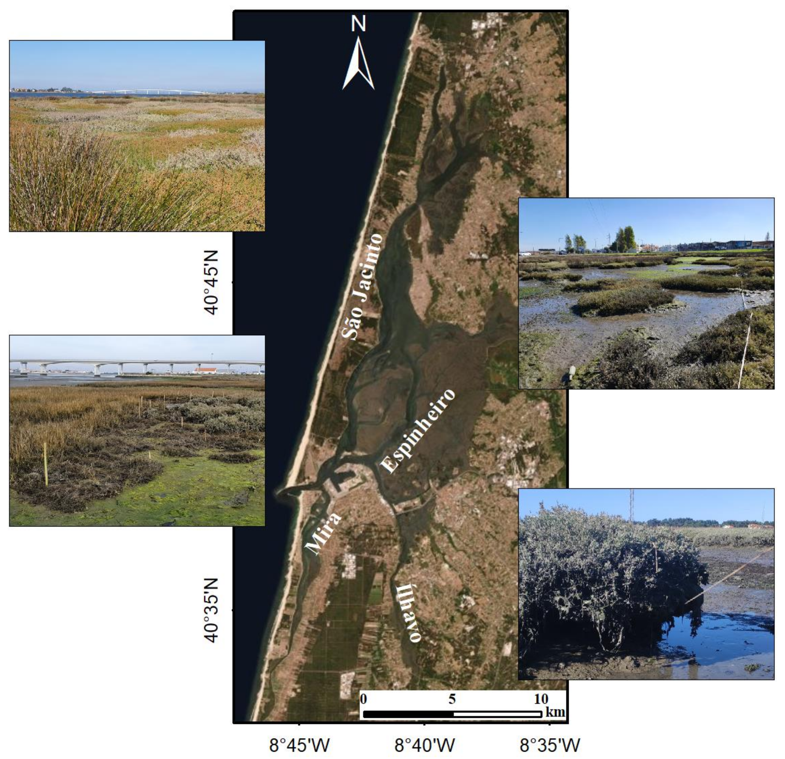
2.1. Study Area

Ria de Aveiro (Figure 1) is a mesotidal lagoon of complex geometry located on the northwest coast of Portugal and connected to the Atlantic Ocean through an artificial inlet [34]. The lagoon encompasses an extensive system with a length and width of 45 and 10 km, respectively, and salt marshes occupy about 50 km2 of the lagoon area [33].
The lagoon’s hydrodynamics is tidally dominated and is primarily regulated by a semidiurnal tide, exhibiting a mean amplitude of 2 m in the entrance, ranging from 0.46 to 3.52 m at neap and spring tides, respectively [35,36,37]. The hydrology differs for each channel based on different tidal prisms and freshwater inputs [38]. The tidal prism for each of the main channels relative to its value at the lagoon mouth is approximately 45%, 25%, 13%, and 9% for the São Jacinto, Espinheiro, Ílhavo, and Mira channels, respectively [39,40].
From its intricate configuration emerges a highly dynamic system both in terms of physical as well as biogeochemical processes [39] and thus, to obtain a broader sample of the different conditions, this study took place in three salt marshes, each located at different main channels: Mira, São Jacinto, and Ílhavo (Figure 1).

2.2. Field Data Collection and Laboratory and Numerical Analysis

A multidisciplinary approach was employed to achieve the goals of this study, resorting to robust and consistent direct field measurements. A plan was outlined for the execution of field campaigns at each of the selected salt marshes of the 3 main channels. The field sampling was conducted monthly, between October 2021 and September 2022, at low water spring tides to ensure more accessibility and manipulation time.
In the days following the fieldwork, the collected samples were analyzed in the laboratory, and hydrodynamic variables were determined using a numerical model (Table 1). The research design was divided into two complementary analyses: initial characterization and inventorying of the salt marshes, followed by a study of the environmental, physicochemical, and hydrodynamic parameters associated with their respective main species’ monospecific patches (Table 1).

2.2.1. Characterization and Inventorying of the Transects

In the first stage, a single permanent transect perpendicular to the main channel was established in the most extensive areas that presented adequate terrestrial accessibility (as they had to be surveyed by foot) and with the most overall coverage at each site in accordance with the previous field assessments in the context of this investigation, which was also based on a predefined permanent transect in Mira that we meant to monitor. The transects’ topographic profile, z(m), was then registered using the Trimble R8s GNSS system (Table 1) and the soil elevation data was later used to determine hydrodynamic variables according to the procedure explained in Section 2.2.3.
Quadrats were initially placed at the very beginning of the transects (at their highest elevation points as delimited by upward roads, at the furthest end from the water channel) and moved forward a meter at a time with its right side aligned with the soil elevation points that were measured. A total of 120, 50, and 70 m2 were surveyed every month in Mira, São Jacinto, and Ílhavo, respectively. Each species was identified and had its cover-abundance determined according to the Braun-Blanquet (B-B) cover-abundance scale (+ to 5) [42] and as a complement, the average coverage (AC) values attained by each species within the total sampled area of the transects were also calculated [43]:
A C ( % ) = T o t a l   c o v e r T o t a l   s a m p l e d   a r e a
Once gathered, species distribution data were then used to calculate an elevation-dependent Shannon’s entropy, S(z), for intervals within the full range of elevation of all three salt marsh transects [28]:
S z =     i = 1 N P i z ln P i   z
where N is the total number of species in the salt marsh and P i ( z ) is the probability that the ith species be in the established elevation interval.

2.2.2. A Study of the Main Species Monospecific Stands

To better understand the interaction between abiotic variables and species distribution, we selected lower areas of monospecific patches of the three most dominant main shared species between the three salt marshes and performed monthly measurements of environmental, physicochemical, and hydrodynamic variables at five arbitrary sampling points at least 1 m apart (Table 1).
Measurements of the physicochemical parameters were either taken directly in situ (redox potential) or obtained through the collection of sediment samples near the roots of the main species that later went under laboratory analysis (porewater salinity/pH and water content) (Table 1).

2.2.3. Numerical Analysis

A numerical model previously developed and calibrated for the Ria de Aveiro lagoon [43] was used to determine hydrodynamic variables relevant to the establishment of halophytic vegetation (Table 1). A numerical simulation covering the annual period in which the campaigns took place, from 1 October 2021 to 31 September 2022, was performed, and sea surface elevation time series outputted at the nearest point of each salt marsh were considered. In detail, sea surface elevation and soil elevation were combined to identify when each point emerged or submerged, and to determine the hydrodynamic variables:
1.
The mean flood duration (FD), which denotes the time in hours during which the sampling point is flooded [28], was calculated:
F D = i = 1 n d i / n
where d i is the duration of a single flood and n is the number of floods.
2.
The frequency of flooding (F), which estimates the average number of floods that occurred during a reference interval of time [28], was determined:
F =   n / T τ   × 100
where n represents the number of floods and T τ is the time elapsed between surveys.
3.
The water depth (WD), defined as the difference between the level of mean high water (MHW) and soil elevation, z, was calculated [44]:
W D = M H W z
The hydrodynamic variables were determined every month for the monospecific stands considering the sea surface elevation covering the time between each campaign, while for the topographic profile, the hydrodynamic variables were calculated considering the sea surface elevation annual time series. The annual time series were also used to determine several tidal levels for each salt marsh, namely the highest tidal level (HL), the mean high water springs (MHWS), the mean high water (MHW), the mean high water neaps (MHWN), and the mean sea level (MSL).

2.3. Statistical and Data Analysis

Collected data about the topographic profiles, the tidal levels, and the vegetation survey of the chosen transects were compiled to determine the ranges of soil elevation and hydroperiod variables in which the different salt marsh species were preferentially distributed. To determine the influence of the environmental, physicochemical, and hydrodynamic data collected, a principal component analysis (PCA) was performed with their normalized values using the “ggbiplot” [45] and “ggfortify” [46] packages in RStudio (Versions 4.1.3 and 4.2.2). The data were then complemented with a permutational multivariate analysis of variance (PERMANOVA) using Euclidean distances as a measure of resemblance on PRIMER (version 7). Differences were considered significant at a p-value of <0.05.

3. Results

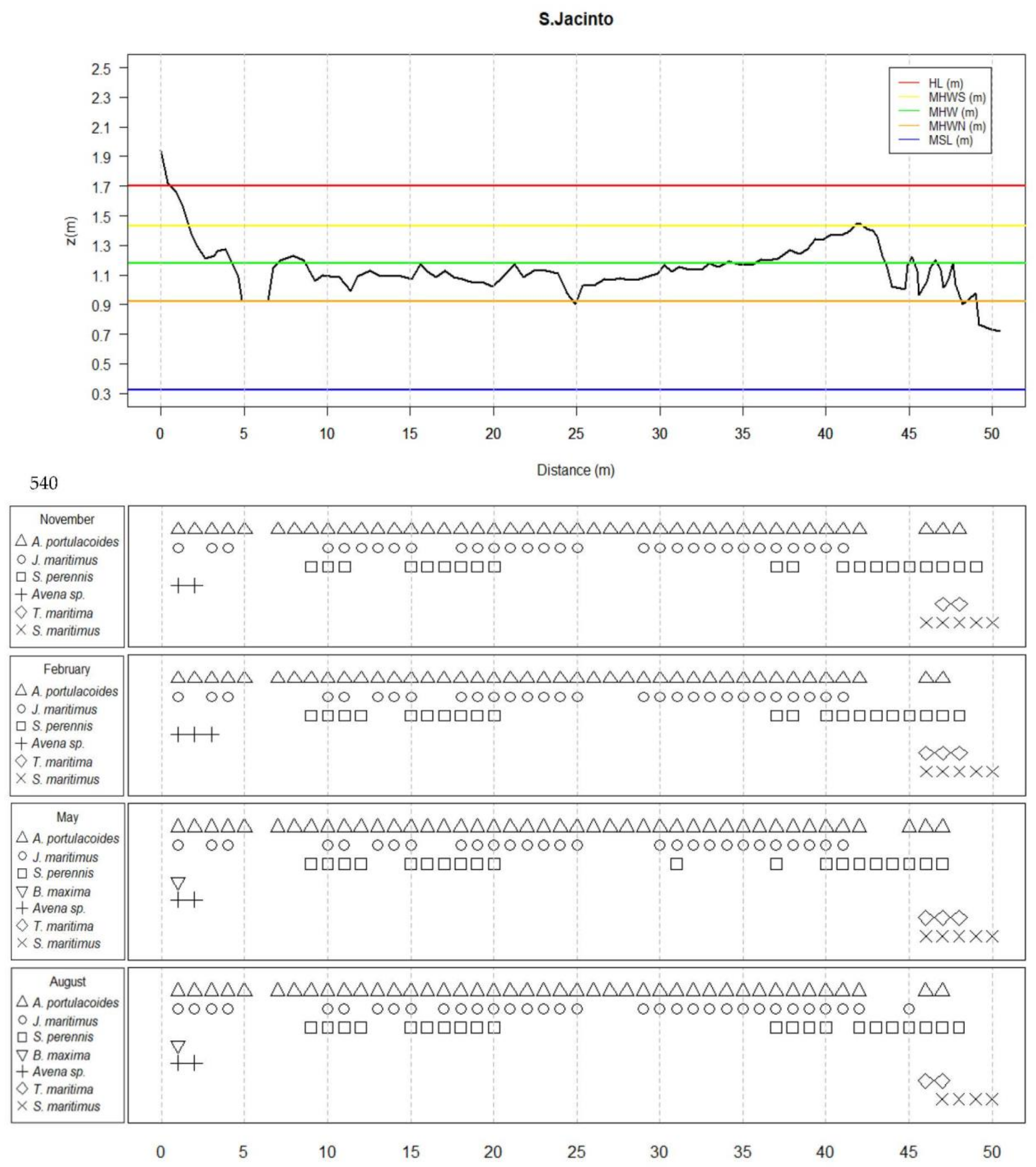
3.1. Species Distribution along the Transects

Of the salt marshes studied, Mira’s salt marsh was the most distinctive in all its dimensions. As shown in Figure 2, Figure 3 and Figure 4 this site presented the most typical zonation configuration, with distinct low, middle, and high marsh regions. Moreover, with Mira’s channel being the closest to the inlet, the selected transect at this site was the most influenced by the tides, which induced up to 1.79 m of sea surface elevation (Figure 2).
The wider range of elevations and greater length of Mira’s transect was matched by a broader array of species—thirteen in total over the year (See Appendix A, Table A1)—ranging from sub-shrubby halophytic species, such as Atriplex portulacoides L., Salicornia perennis Mill., to several herbaceous species, such as Juncus maritimus Lam., Sporobolus versicolor (E.Fabre) P.M.Peterson and Saarela, Puccinellia maritima (Huds.) Parl., and Elymus repens (L.) Gould, and even invasive species, such as Carpobrotus edulis (L.) N.E.Br.
São Jacinto’s salt marsh displayed a broad topographic profile like Mira’s, though with less noticeable boundaries (Figure 3); however, it attained far fewer species, a total of seven along the different seasons, an amount closer to the eight species identified at Ílhavo, where the transect was marked by several creeks and small-scale elevation fluctuations and was largely confined to the levels of MHWN and MHW. (Figure 4) (See Appendix A, Table A1).
When monitoring these communities, almost no changes in species composition were observed throughout the sampled months (hence, the choice of only representing November’s survey), with the most noticeable differences conveying the appearance and subsequent disappearance of annuals, such as Salicornia europaea L., Atriplex patula L., and Briza maxima L., or the occasional expansion of neighboring species into the sampled areas, namely Phragmites australis (Cav.) Trin. ex Steud.
All three locations (Figure 2, Figure 3 and Figure 4) were mainly dominated by patches of A. portulacoides, S. perennis, and J. maritimus from elevated to lower marsh zones, and patches of S. maritimus in the intermediate and lower areas (except at Ílhavo’s salt marsh, where this species occurred sparingly).
Likewise, the species cover-abundance (Table 2) showed a pattern concomitant to a wider distribution. For all three salt marshes, species that showed broader distributions, namely S. perennis., J. maritimus, A. portulacoides, and S. maritimus, were also the ones with higher coverage and abundance values.
Of these four main species (Table 2), A. portulacoides was the most exuberant species, especially in São Jacinto’s salt marsh, where it covered a big portion of the transect (up to 79.10% of the 50 m2 surveyed). This species is not only abundant but also showed marked dominance, as evidenced by the highest mean Braun-Blanquet scale scores (e.g., 4.48 in São Jacinto).
For the most part, species at São Jacinto and Ílhavo exhibited higher Braun-Blanquet scores due to a greater dominance and the formation of larger almost monospecific stands, contrasting with Mira’s marsh communities, which generally presented lower Braun-Blanquet scores (Table 2) because although this latter marsh had the greatest extent, its species were often found in multispecific stands.
Accordingly, as observed in Figure 5, entropy displayed higher values at mid-elevation intervals in all three studied locations, but especially at Mira’s salt marsh. Overall, communities were more diverse at intermediate levels of altitudes of each salt marsh. It is interesting to note that the maximum Shannon Entropy values are reached at 1.45 m elevation in Mira and Ílhavo (which coincides with the level of MHSW), and this value decreases to 0.9 in Ílhavo coinciding with the level of MHWN.
Lastly, a closer look into the main species distribution along the transects (Figure 6) showed that A. portulacoides was the species found in the broadest range of soil elevation at elevations ranging from 0.45 to 1.94 m. It prevailed in intervals varying from 1 to 1.3 m of elevation at Ílhavo and São Jacinto, and from 1.6 to 1.9 m in Mira. Regarding S. perennis and J. maritimus, these species were found in a lesser extent of soil elevation ranges, mainly in the low to mid ranges (0.7 to 1.9 m), and S. maritimus was mostly settled in even lower areas with minor soil elevation (0.4 to 0.7 m).

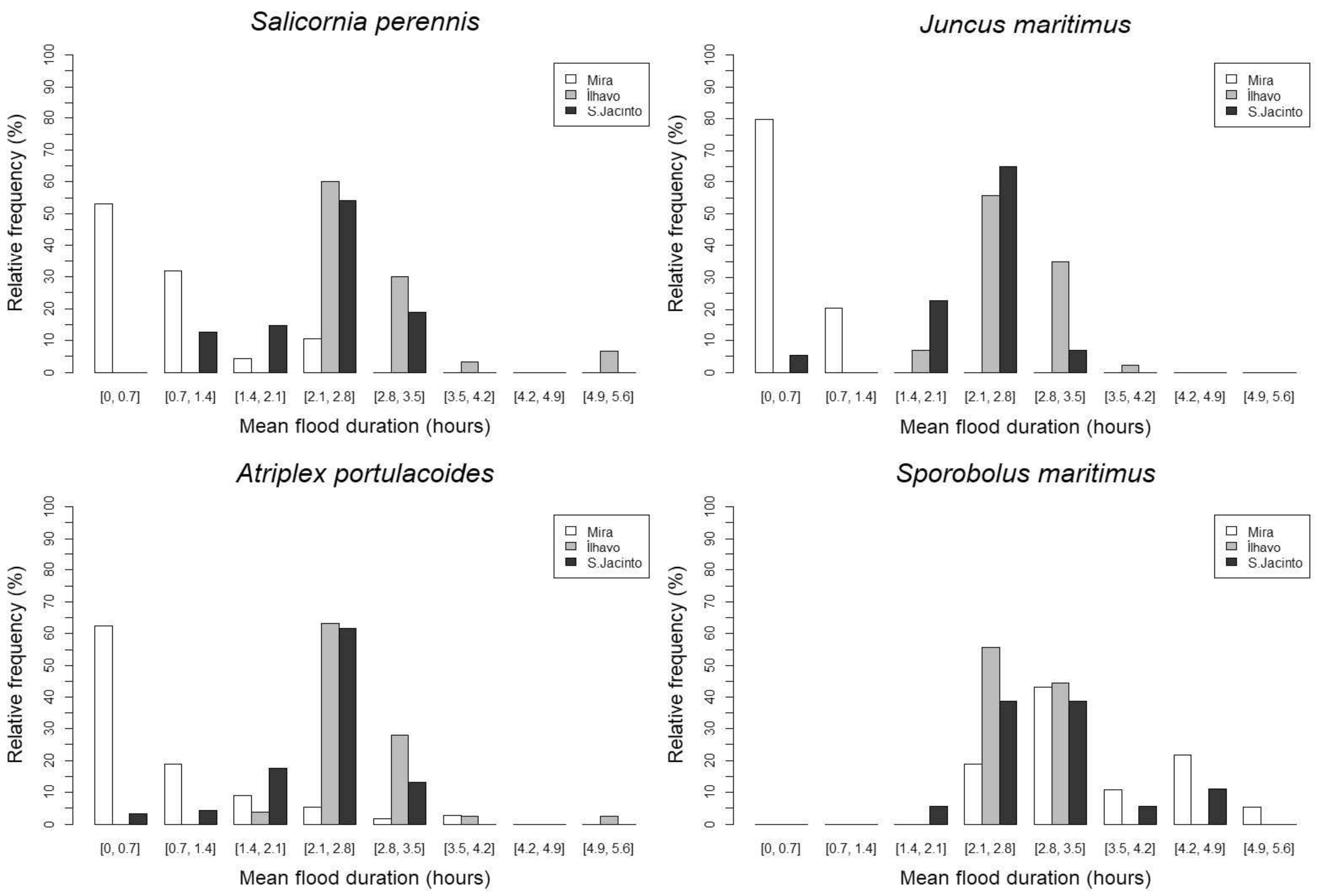
3.2. Main Species Distribution

According to the PCA analysis, the first two components contain 68.70% of the global variation. The first component accounts for 53.86% of the global variation, while the second explains only 14.84%. As illustrated in Figure 7, Axis 1 has a strong positive loading for the soil elevation and soil water content variables, and strong negative loadings for the mean flood duration, frequency of flooding, and water depth, whereas Axis 2 is influenced by strong positive loadings for salinity and inversely by the redox potential. As a result, this analysis points toward a negative correlation between the hydrodynamic variables, soil elevation, and water content, and similarly, between the redox potential and salinity.
A further assessment of this analysis, in conjugation with the complementary PERMANOVA analysis, revealed significative differences in variance between species, salt marshes, and most of their joint interaction (p-value < 0.05; Table 3). The data suggests a marked distinction between the distribution of S. maritimus and the other two studied species. Although, within a broad range of values, S. maritimus tended to be in lower areas subjected to a higher frequency of flooding, extended mean flood duration, and deeper water depth, typically, with reduced soil water content and slightly more reduced redox potential. S. perennis, on the other hand, inhabited regions with intermediate values of altitude subjected to the widest variance in most of the examined parameters. Lastly, in opposition to the other species under investigation, the studied variables linked to A. portulacoides exhibited a reduced range of variation, and the variability that occurred appeared to be more correlated to seasonal changes in salinity and redox potential.

4. Discussion

4.1. Salt Marsh Monitoring and Characterization

In the study of the three different transects, we found that the selected salt marshes shared a core set of flora comprised S. perennis, A. portulacoides, J. maritimus, and S. maritimus (Figure 2, Figure 3 and Figure 4). The observed communities were consonant with the halophytic-rich ones commonly found at temperate latitudes, where there is usually a prominent dominance of herbaceous species [1,47,48], and although less common in northern salt marshes, the dominance of sub-shrubby species such as A. portulacoides and S. perennis is also in agreement with earlier findings at the lower limit of the temperate floristic cluster where our study area is situated [1,48].
Overall, the floristic communities at the study sites evidenced very few changes over the year, and the changes that occurred were related either to the emergence and subsequent disappearance of annual species or coverage adjustments seemingly related to flowering periods of certain species. Notice that higher cover-abundance values of the main species overlapped with their respective flowering period, ranging from August to November for A. portulacoides and S. perennis, July to September for S. maritimus, and May to July for J. maritimus, as shown in Figure A1, Figure A2 and Figure A3.
Likewise, when set against previous data collected from salt marshes at Mira’s channel (December 1995 to December 1996) [49] and with other unpublished data (May 2010 and January 2011) collected by us, our results showed that although this region has been subjected to degradation, changes in vegetation cover, and loss of area [33], there has been only some slight changes in its communities composition over the past two decades. Overall, the main differences between the four sampled periods illustrated the disappearance of S. europaea beyond the years sampled by Silva [49] (though understandably so given this species’ pioneer status and annual character) and the observed emergence of S. versicolor in 2010 and E. repens and C. edulis in 2021. Moreover, just like in this investigation, S. perennis, A. portulacoides, J. maritimus, and S. maritimus were the most abundant species (although not always following the same proportions).
We also found that communities were more even, diverse, and less dominated by a particular species at the intermediate levels of altitude of each salt marsh (Figure 5), where intermediate values of inundation periods and frequency, as well as water depth, were typically found, possibly because these latter hydrodynamic parameters could have ultimately acted as disruptive forces—since they are usually associated with salinity and oxidative stresses and the deposition of potentially damaging debris [1,50]—especially in lower elevations where they were more prominent (as illustrated by Figure 6 and Figure A4, Figure A5 and Figure A6), but any further considerations about this possibility should ideally be investigated in the future within more sampling sites.
Similarly, as illustrated in Figure 5, diversity was particularly higher at Mira’s salt marsh; however, this study site was located in one of the least deteriorated areas of Ria de Aveiro [33], and as such, it presented a greater length as well as greater ranges of elevation, which conceivably promoted new opportunities for the establishment of additional species (Figure 2) not as adapted to the more restrictive environmental conditions found within the other salt marshes that were degraded and characterized by less soil elevation and more inundation (Figure 1, Figure 3, and Figure 4).
Furthermore, at Mira, S. perennis, A. portulacoides, and J. maritimus were found at slightly higher elevation intervals (Figure 6), while S. maritimus was compelled to even lower more stressful surroundings despite the greatest elevation ranges found in this study site (Figure 2). The preceding strongly suggests that the occurrence of the different new species likely changed the dynamic between species competition and/or facilitation interactions, which are known to be frequent in disturbed environments [51,52].
Such competitive interactions at salt marshes are usually associated with a trade-off between competition and physiological tolerances, which posits that more elevated and less stressful intertidal zones are typically occupied by stronger competitors who ultimately limit the upper boundaries of the weak competitors to lower stressful physical environments [27,30,50,53,54]. Therefore, it is reasonable to determine that from the observed core species, A. portulacoides was the most competitively dominant species and S. maritimus the least. This assertion is further supported by one other investigation [55], where the authors, while following both a young and a mature salt marsh, verified that A. portulacoides largely colonizes and dominates most of the middle marsh areas, displacing species such as S. perennis and S. maritimus (common to our study) to lower elevations.
The observed dominance of A. portulacoides was most certainly related to its ability to form denser stands that make it difficult to coexist with other species [56]. However, as evidenced in our results and in [55], not even the robust morphology of this species could prevent the later invasion of taller and much more competitive species when the conditions become favorable. Eventually, plants with C4 photosynthetic pathways, such as E. repens and S. versicolor (found in Mira), outcompete C3 species, such as A. portulacoides and S. perennis, that have slower rates of biomass production and thus a more limited ability to grow rapidly and are usually less efficient in the use of available nitrogen and water [1,57,58].

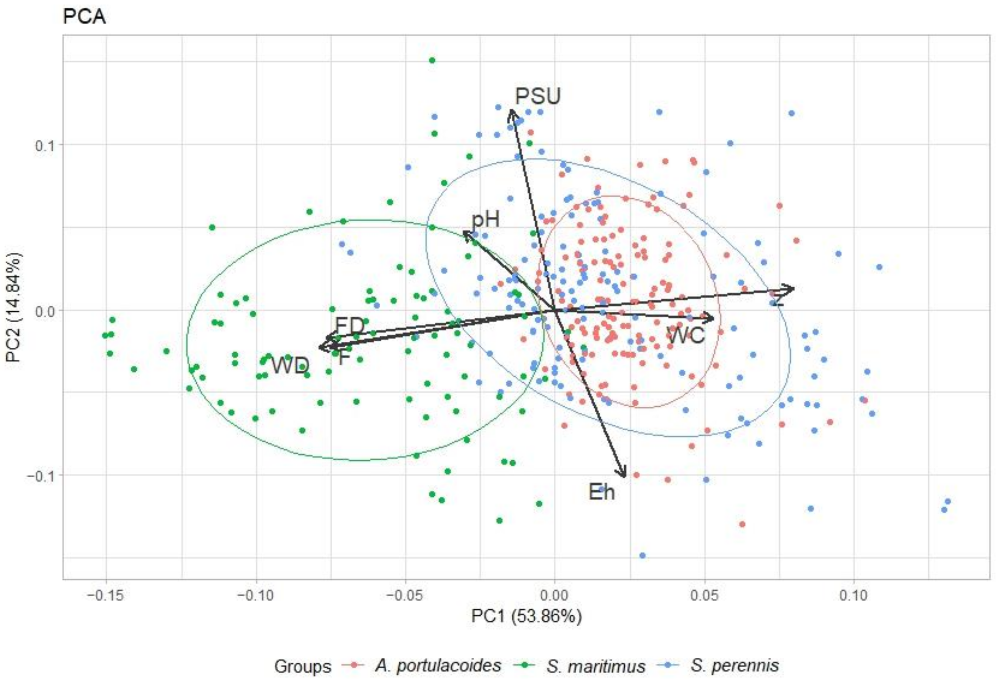
4.2. Biotic and Abiotic Factors versus Vegetation Monospecific Stands

Although Juncus maritimus was one of the four species common to all three salt marshes, it was rarely found in patches like the other three: Atripex portulacoides, Sporobolus maritimus, and Salicornia perennis, but was rather characterized by many solitary specimens often found mixed with other species. As a result, this species was omitted from the smaller-scale study of monospecific stands, as there was no viable way of obtaining the intended environmental, physicochemical, and hydrodynamic variables in exclusive association with Juncus maritimus.
Nevertheless, the analysis of the available monospecific stands of the other main species further highlighted the occurrence of a possible competition/tolerance trade-off. Even in a smaller scale of elevation ranges, the differences in species distribution and along the several measured variables were significantly distinct (Table 3). A. portulacoides, which does not develop aerenchyma [59], favored higher elevations and areas closer to creekbanks, likely as a response to better conditions of aeration and nitrogen availability at such sites, as was later evidenced by the typically higher redox values of sediment in which this species was found. As a better competitor, A. portulacoides ultimately compelled the other main species into lower elevations with greater instability and more stressful conditions (Figure 7).
Furthermore, the PCA analysis suggested that the inundation variables were within what would be predictable at the different elevation ranges [1], as the highest flood durations, frequencies, and water depths were effectively found at sampling points with lower altitudes (Figure 7). However, contrarily to previous assessments, lower redox values, although concurrent to lower elevations subjected to greater influence by the tides [30,60,61], did not necessarily match more waterlogged sediments (Figure 7) that are usually expected to have less oxygen available [20,62].
The observed greater waterlogging at upper elevations could either have resulted from better drainage at lower sites closer to the edge [63], especially at Mira’s salt marsh where sediment was sandier and more permeable [64], or essentially portrayed the crucial influence exerted by vascular plants on their surroundings [8]. It has become clear that the redox potential can be effected by different root systems/anatomies and/or metabolic activities [65,66,67]. For instance, greater metabolic activity of grasses (such as S. maritimus) coupled with elevated evapotranspiration rates has been linked to sediment oxidation [68,69] and thus may explain these observations.
Lastly, although recognized as some of the major delimiting factors of vegetation establishment [1], pH and salinity did not appear to substantially influence species distribution where monospecific stands were more prominent, as most of the data variation stemmed from differences in topography and hydrodynamics (Figure 7).

5. Conclusions

Our results showed that, of the abiotic factors deemed as the main delimiting forces of salt marsh vegetation, the soil elevation and hydroperiod were the most restrictive factors influencing the structuring of the floristic communities of Ria de Aveiro’s salt marshes, as they ultimately influenced the biotic interactions and accounted for most of the variation observed between the studied monospecific stands.
Although the authors recognize that this study would have benefited from more sampling areas, based on the monitoring of the chosen study sites, it can be stated that species composition is typically more diversified and can remain unchanged for long periods of time in areas with slower degradation and loss of area, while areas with more degradation and/or less extension presented less coverage and less diversity of species.
As such, since the topography and hydroperiod displayed such a big impact on habitat delimitation and vegetation composition, we suggest that in the future, when attempting to identify areas with greater potential for salt marsh restoration and/or conservation, researchers should start by identifying areas with favorable topographic and hydrodynamic settings or areas that at least have the potential to be expanded in length and/or altitude.
Lastly, it would be relevant to complement this investigation with future research on the factors that ultimately influence salt marsh elevation and hydroperiods, such as accretion and changes in mean sea level, so that, in conjunction with the obtained results on species distribution, better predictions regarding the adaptation of marshes to climate change could be made.

Author Contributions

Conceptualization, M.M.G., C.L.L. and H.S.; methodology, M.M.G., C.L.L. and H.S.; software, C.L.L., A.S.R. and J.M.D.; validation, A.S.R. and J.M.D.; formal analysis, M.M.G., C.L.L. and H.S.; investigation, M.M.G., C.L.L. and H.S.; resources, H.S. and C.L.L.; data curation, M.M.G., N.N.M., C.L.L., A.S.R., J.M.D. and H.S.; writing—original draft preparation, M.M.G.; writing—review and editing, M.M.G., N.N.M., C.L.L., H.S., A.S.R. and J.M.D.; visualization, M.M.G.; supervision, H.S. and C.L.L.; project administration, H.S.; funding acquisition, H.S. All authors have read and agreed to the published version of the manuscript.

Funding

This research received support from PT national funds (FCT/MCTES, Fundação para a Ciência e Tecnologia, and Ministério da Ciência, Tecnologia e Ensino Superior) through the projects UIDP/50017/2020 + UIDB/50017/2020 + LA/P/0094/2020 (CESAM). The third author is funded by national funds through the Portuguese Science Foundation (FCT) under project CEECIND/00459/2018.

Institutional Review Board Statement

Not applicable.

Informed Consent Statement

Not applicable.

Data Availability Statement

Not applicable.

Acknowledgments

Thanks are due to Aldiro Pereira and Ana Clara Donati for all the support with the field campaigns.

Conflicts of Interest

The authors declare no conflict of interest.

Appendix A

The initial plan was to collect and analyze data from October 2021 to September 2022, but due to some mishaps along the way with some methodologies and measuring instruments, some of the physicochemical and hydrodynamic variables ended up incomplete. For that reason, the data used for the PCA and PERMANOVA statistical analysis ended up referring only to the last ten months of the studied period, extending from December 2021 to September 2022.
Table A1. Summary table with the mean overall coverage-abundance Braun-Blanquet (B-B) and average cover (AC) values attained by all the species encountered throughout the year (and their respective standard deviation). Scientific names according to POWO (https://powo.science.kew.org/, accessed on 25 January 2023). The symbol “+” refers to low coverage with few individuals.
SpeciesCover-Abundance
MiraSão JacintoÍlhavo
MonthsB-BACMonthsB-BACMonthsB-BAC
Salicornia perennisOct–Aug3.33 ± 1.0215.97 ± 2.24Oct–Aug3.24 ± 1.0919.63 ± 1.13Oct–Aug3.86 ± 1.0115.99 ± 1.33
Juncus maritimusOct–Aug3.12 ± 0.9725.33 ± 1.00Oct–Aug2.33 ± 0.9417.42 ± 0.84Oct–Aug3.49 ± 0.9215.99 ± 1.62
Atriplex
portulacoides
Oct–Aug2.86 ± 1.0733.64 ± 2.71Oct–Aug4.22 ± 0.8378.31 ± 0.50Oct–Aug3.48 ± 1.1139.7 ± 1.50
Sporobolus
maritimus
Oct–Aug3.41 ± 0.8720.75 ± 1.52Oct–Aug2.99 ± 0.682.66 ± 0.60Oct–Aug+0.61 ± 0.16
Sporobolus
versicolor
Oct–Aug2.90 ± 1.1413.95 ± 2.84
Elymus repensOct–Aug3.23 ± 1.2518.91 ± 4.06
Carpobrotus edulisOct–Aug3.45 ± 0.702.41 ± 0.50
Limbarda
crithmoides
Oct–Aug1.96 ± 0.510.61 ± 0.23
Puccinellia
maritima
Nov–Aug2.54 ± 0.892.37 ± 1.13
Spergularia marinaNov–Aug+0.12 ± 0.06
Tripolium
pannonicum
Oct–May+0.20 ± 0.15
Limonium vulgareMay–Aug+0.04 ± 0.01
Avena sp.Oct–Aug3.56 ± 0.000.72 ± 0.35Oct–Aug3.41 ± 0.543.47 ± 0.29
Briza maxima May–Aug+0.17 ± 0.04
Triglochin maritima Nov–Aug3.46 ± 0.411.02 ± 0.23Apr–May3.00 ± 0.000.36 ± 0.02
Salicornia europaea Oct–Nov
Jul–Aug
3.5 ± 0.000.13 ± 0.04
Atriplex patula Nov3.00 ± 0.000.06 ± 0.00
Phragmites australis Oct
Jul–Aug
3.00 ± 0.000.30 ± 0.19
Figure A1. Topographic profile of Mira´s salt marsh and its respective tidal levels. HL (highest tidal level), MHWS (mean high water springs), MHW (mean high water), MHWN (mean high water neaps), MSL (mean sea level). Representation of vegetation distribution through the length of the transept (autumn: November, winter: February, spring: May, summer: August).
Applsci 13 04605 g0a1
Figure A2. Topographic profile of São Jacinto´s saltmarsh and its respective tidal levels. HL (highest tidal level), MHWS (mean high water springs), MHW (mean high water), (mean high water neaps), MSL (mean sea level). Representation of vegetation distribution through the length of the transept (autumn: November, winter: February, spring: May, summer: August).
Applsci 13 04605 g0a2
Figure A3. Topographic profile of Ílhavo´s salt marsh and its respective tidal levels. HL (highest tidal level), MHWS (mean high water springs), MHW (mean high water), MHWN (mean high water neaps), MSL (mean sea level). Representation of vegetation distribution through the length of the transept (autumn: November, winter: February, spring: May, summer: August).
Applsci 13 04605 g0a3
Figure A4. Mean flood duration (FD (hours)). Relative frequency distribution of the main species regarding the mean flood duration for each of the studied marshes.
Applsci 13 04605 g0a4
Figure A5. Water depth (WD (m)). Relative frequency distribution of the main species regarding the water depth for each of the studied marshes.
Applsci 13 04605 g0a5
Figure A6. Frequency of flooding (F (%)). Relative frequency distribution of the main species regarding the frequency of flooding percentage for each of the studied marshes.
Applsci 13 04605 g0a6

References

  1. Adam, P. Saltmarsh Ecology; Cambridge University Press: Cambridge, UK, 1990; ISBN 0521245087. [Google Scholar]
  2. Adam, P. Saltmarshes in a Time of Change. Environ. Conserv. 2002, 29, 39–61. [Google Scholar] [CrossRef]
  3. Barbier, E.B.; Hacker, S.D.; Kennedy, C.; Koch, E.W.; Stier, A.C.; Silliman, B.R. The Value of Estuarine and Coastal Ecosystem Services. Ecol. Monogr. 2011, 81, 169–193. [Google Scholar] [CrossRef]
  4. Sousa, A.I.; Santos, D.B.; Da Silva, E.F.; Sousa, L.P.; Cleary, D.F.R.; Soares, A.M.V.M.; Lillebø, A.I. “Blue Carbon” and Nutrient Stocks of Salt Marshes at a Temperate Coastal Lagoon (Ria de Aveiro, Portugal). Sci. Rep. 2017, 7, srep41225. [Google Scholar] [CrossRef] [PubMed] [Green Version]
  5. Chmura, G.L.; Anisfeld, S.C.; Cahoon, D.R.; Lynch, J.C. Global Carbon Sequestration in Tidal, Saline Wetland Soils. Global Biogeochem. Cycles 2003, 17, 1111. [Google Scholar] [CrossRef]
  6. Owers, C.J.; Woodroffe, C.D.; Mazumder, D.; Rogers, K. Carbon Storage in Coastal Wetlands Is Related to Elevation and How It Changes over Time. Estuar. Coast. Shelf Sci. 2022, 267, 107775. [Google Scholar] [CrossRef]
  7. Vernberg, F.J. Salt-marsh Processes: A Review. Environ. Toxicol. Chem. 1993, 12, 2167–2195. [Google Scholar] [CrossRef]
  8. Sarika, M.; Zikos, A. Coastal Salt Marshes. In Handbook of Halophytes; Grigore, M.-N., Ed.; Springer: Cham, Switzerland, 2020; pp. 1–39. [Google Scholar]
  9. King, S.E.; Lester, J.N. The Value of Salt Marsh as a Sea Defence. Mar. Pollut. Bull. 1995, 30, 180–189. [Google Scholar] [CrossRef]
  10. Gedan, K.B.; Kirwan, M.L.; Wolanski, E.; Barbier, E.B.; Silliman, B.R. The Present and Future Role of Coastal Wetland Vegetation in Protecting Shorelines: Answering Recent Challenges to the Paradigm. Clim. Change 2011, 106, 7–29. [Google Scholar] [CrossRef]
  11. Shepard, C.C.; Crain, C.M.; Beck, M.W. The Protective Role of Coastal Marshes: A Systematic Review and Meta-Analysis. PLoS ONE 2011, 6, e27374. [Google Scholar] [CrossRef]
  12. Anderson, M.E.; Smith, J.M. Wave Attenuation by Flexible, Idealized Salt Marsh Vegetation. Coast. Eng. 2014, 83, 82–92. [Google Scholar] [CrossRef]
  13. Gedan, K.B.; Silliman, B.R.; Bertness, M.D. Centuries of Human-Driven Change in Salt Marsh Ecosystems. Ann. Rev. Mar. Sci. 2009, 1, 117–141. [Google Scholar] [CrossRef] [Green Version]
  14. Fitzgerald, D.M.; Hughes, Z. Marsh Processes and Their Response to Climate Change and Sea-Level Rise. Annu. Rev. Earth Planet. Sci. 2019, 47, 481–517. [Google Scholar] [CrossRef] [Green Version]
  15. Fagherazzi, S.; Mariotti, G.; Leonardi, N.; Canestrelli, A.; Nardin, W.; Kearney, W.S. Salt Marsh Dynamics in a Period of Accelerated Sea Level Rise. J. Geophys. Res. Earth Surf. 2020, 125, e2019JF005200. [Google Scholar] [CrossRef]
  16. Timmerman, A.; Haasnoot, M.; Middelkoop, H.; Bouma, T.; McEvoy, S. Ecological Consequences of Sea Level Rise and Flood Protection Strategies in Shallow Coastal Systems: A Quick-Scan Barcoding Approach. Ocean Coast. Manag. 2021, 210, 105674. [Google Scholar] [CrossRef]
  17. Crosby, S.C.; Sax, D.F.; Palmer, M.E.; Booth, H.S.; Deegan, L.A.; Bertness, M.D.; Leslie, H.M. Salt Marsh Persistence Is Threatened by Predicted Sea-Level Rise. Estuar. Coast. Shelf Sci. 2016, 181, 93–99. [Google Scholar] [CrossRef] [Green Version]
  18. Davy, A.J. Development and Structure of Salt Marshes: Community Patterns in Time and Space. In Concepts and Controversies in Tidal Marsh Ecology; Springer: Cham, Switzerland, 2005; pp. 137–156. [Google Scholar] [CrossRef]
  19. Rogers, K.; Woodroffe, C.D. Tidal Flats and Salt Marshes. In Coastal Environments and Global Change; John Wiley & Sons, Ltd.: Hoboken, NJ, USA, 2015; pp. 227–250. ISBN 9781119117261. [Google Scholar]
  20. Pennings, S.C.; He, Q. Community Ecology of Salt Marshes. In Salt Marshes; FitzGerald, D., Hughes, Z., Eds.; Cambridge University Press: Cambridge, UK, 2021; pp. 82–112. [Google Scholar]
  21. Gao, S. Geomorphology and Sedimentology of Tidal Flats. In Coastal Wetlands: An Integrated Ecosystem Approach; Perillo, G.M.E., Wolanski, E., Cahoon, D.R., Hopkinson, C.S., Eds.; Elsevier B.V.: Amsterdam, The Netherlands, 2018; pp. 359–381. ISBN 9780444638939. [Google Scholar]
  22. Hughes, Z.J.; FitzGerald, D.M.; Wilson, C.A. Impacts of Climate Change and Sea Level Rise. In Salt Marshes; FitzGerald, D., Hughes, Z., Eds.; Cambridge University Press: Cambridge, UK, 2021; pp. 476–481. [Google Scholar]
  23. Day, J.; Burdick, D.M.; Ibáñez, C.; Mitsch, W.J.; Elsey-Quirk, T.; Rivaes, S. Restoration of Tidal Marshes. In Salt Marshes; FitzGerald, D., Hughes, Z., Eds.; Cambridge University Press: Cambridge, UK, 2021; pp. 443–475. [Google Scholar]
  24. Townend, I.; Fletcher, C.; Knappen, M.; Rossington, K. A Review of Salt Marsh Dynamics. Water Environ. J. 2011, 25, 477–488. [Google Scholar] [CrossRef]
  25. Temmerman, S.; Bouma, T.J.; Govers, G.; Wang, Z.B.; De Vries, M.B.; Herman, P.M.J. Impact of Vegetation on Flow Routing and Sedimentation Patterns: Three-Dimensional Modeling for a Tidal Marsh. J. Geophys. Res. Earth Surf. 2005, 110. [Google Scholar] [CrossRef] [Green Version]
  26. Costa, C.; Marangoni, J.C.; Azevedo, A.M.G. Plant Zonation in Irregularly Flooded Salt Marshes: Relative Importance of Stress Tolerance and Biological Interactions. J. Ecol. 2003, 91, 951–965. [Google Scholar] [CrossRef]
  27. Pennings, S.C.; Grant, M.B.; Bertness, M.D. Plant Zonation in Low-Latitude Salt Marshes: Disentangling the Roles of Flooding, Salinity and Competition. J. Ecol. 2005, 93, 159–167. [Google Scholar] [CrossRef]
  28. Silvestri, S.; Defina, A.; Marani, M. Tidal Regime, Salinity and Salt Marsh Plant Zonation. Estuar. Coast. Shelf Sci. 2005, 62, 119–130. [Google Scholar] [CrossRef]
  29. Chapman, V. Salt Marshes and Salt Deserts of the World. In Ecology of Halophytes; Reimold, R., Queen, W., Eds.; Academica Press, Inc.: London, UK, 1974; pp. 3–19. ISBN 0-12-586450-7. [Google Scholar]
  30. Ungar, I.A. Are Biotic Factors Significant in Influencing the Distribution of Halophytes in Saline Habitats? Bot. Rev. 1998, 64, 176–199. [Google Scholar] [CrossRef]
  31. Guo, H.; Pennings, S.C. Mechanisms Mediating Plant Distributions across Estuarine Landscapes in a Low-Latitude Tidal Estuary. Ecology 2012, 93, 90–100. [Google Scholar] [CrossRef] [PubMed] [Green Version]
  32. Lee, J.S.; Kim, J.W. Dynamics of Zonal Halophyte Communities in Salt Marshes in the World. J. Mar. Isl. Cult. 2018, 7, 84–106. [Google Scholar] [CrossRef]
  33. Lopes, C.L.; Mendes, R.; Caçador, I.; Dias, J.M. Assessing Salt Marsh Loss and Degradation by Combining Long-Term LANDSAT Imagery and Numerical Modelling. Land Degrad. Dev. 2021, 32, 4534–4545. [Google Scholar] [CrossRef]
  34. Dias, J.M.; Picado, A. Impact of Morphologic Anthropogenic and Natural Changes in Estuarine Tidal Dynamics. J. Coast. Res. 2011, 64, 1490–1494. [Google Scholar]
  35. Dias, J.M.; Lopes, J.F.; Dekeyser, I. Hydrological Characterisation of Ria de Aveiro, Portugal, in Early Summer. Oceanol. Acta 1999, 22, 473–485. [Google Scholar] [CrossRef] [Green Version]
  36. Lopes, C.L.; Dias, J.M. Assessment of Flood Hazard during Extreme Sea Levels in a Tidally Dominated Lagoon. Nat. Hazards 2015, 77, 1345–1364. [Google Scholar] [CrossRef]
  37. Dias, J.M.; Pereira, F.; Picado, A.; Lopes, C.L.; Pinheiro, J.P.; Lopes, S.M.; Pinho, P.G. A Comprehensive Estuarine Hydrodynamics-Salinity Study: Impact of Morphologic Changes on Ria de Aveiro (Atlantic Coast of Portugal). J. Mar. Sci. Eng. 2021, 9, 234. [Google Scholar] [CrossRef]
  38. Vaz, N.; Miguel Dias, J.; Leitão, P.C. Three-Dimensional Modelling of a Tidal Channel: The Espinheiro Channel (Portugal). Cont. Shelf Res. 2009, 29, 29–41. [Google Scholar] [CrossRef]
  39. Picado, A.; Dias, J.M.; Fortunato, A.B. Tidal Changes in Estuarine Systems Induced by Local Geomorphologic Modifications. Cont. Shelf Res. 2010, 30, 1854–1864. [Google Scholar] [CrossRef] [Green Version]
  40. Lopes, C.L.; Silva, P.A.; Dias, J.M.; Rocha, A.; Picado, A.; Plecha, S.; Fortunato, A.B. Local Sea Level Change Scenarios for the End of the 21st Century and Potential Physical Impacts in the Lower Ria de Aveiro (Portugal). Cont. Shelf Res. 2011, 31, 1515–1526. [Google Scholar] [CrossRef]
  41. Ribeiro, A.S.; Lopes, C.L.; Sousa, M.C.; Gomez-Gesteira, M.; Dias, J.M. Flooding Conditions at Aveiro Port (Portugal) within the Framework of Projected Climate Change. J. Mar. Sci. Eng. 2021, 9, 595. [Google Scholar] [CrossRef]
  42. Braun-Blanquet, J. Fitosociología. Bases Para El Estudio de Las Comunidades Vegetales; H. Blume: Madrid, Spain, 1979; ISBN 9788472141742. [Google Scholar]
  43. Wikum, D.A.; Shanholtzer, G.F. Application of the Braun-Blanquet Cover-Abundance Scale for Vegetation Analysis in Land Development Studies. Environ. Manag. 1978, 2, 323–329. [Google Scholar] [CrossRef]
  44. Kefelegn, H. Mathematical Formulations for Three Components of Hydroperiod in Tidal Wetlands. Wetlands 2019, 39, 349–360. [Google Scholar] [CrossRef]
  45. Wickham, H. Ggplot2: Elegant Graphics for Data Analysis; Springer-Verlag: New York, NY, USA, 2016. [Google Scholar]
  46. Tang, Y.; Horikoshi, M.; Li, W. Ggfortify: Unified Interface to Visualize Statistical Results of Popular R Packages. R J. 2016, 8, 478–489. [Google Scholar] [CrossRef] [Green Version]
  47. Caçador, I.; Neto, J.M.; Duarte, B.; Barroso, D.V.; Pinto, M.; Marques, J.C. Development of an Angiosperm Quality Assessment Index (AQuA-Index) for Ecological Quality Evaluation of Portuguese Water Bodies—A Multi-Metric Approach. Ecol. Indic. 2013, 25, 141–148. [Google Scholar] [CrossRef]
  48. Costa, J.; Arsénio, P.; Monteiro-Henriques, T.; Neto, C.; Pereira, E.; Almeida, T.; Izco, J. Finding the Boundary between Eurosiberian and Mediterranean Salt Marshes. J. Coast. Res. 2009, 1340–1344. [Google Scholar]
  49. Silva, H. Aspectos Morfológicos e Ecofisiológicos de Algumas Halófitas Do Sapal Da Ria de Aveiro. Ph.D. Thesis, Universidade de Aveiro, Aveiro, Portugal, 2000. [Google Scholar]
  50. Bertness, M.D.; Ellison, A.M. Determinants of Pattern in a New England Salt Marsh Plant Community. Ecol. Monogr. 1987, 57, 129–147. [Google Scholar] [CrossRef]
  51. Hacker, S.D.; Gaines, S.D. Some Implications of Direct Positive Interactions for Community Species Diversity. Ecology 1997, 78, 1990–2003. [Google Scholar] [CrossRef]
  52. Bertness, M.D. Interspecific Interactions among High Marsh Perennials in a New England Salt Marsh. Ecology 1991, 72, 125–137. [Google Scholar] [CrossRef] [Green Version]
  53. Pennings, S.C.; Callaway, R.M. Salt Marsh Plant Zonation: The Relative Importance of Competition and Physical Factors. Ecology 1992, 73, 681–690. [Google Scholar] [CrossRef]
  54. Crain, C.M.; Silliman, B.R.; Bertness, S.L.; Bertness, M.D. Physical and Biotic Drivers of Plant Distribution across Estuarine Salinity Gradients. Ecology 2004, 85, 2539–2549. [Google Scholar] [CrossRef] [Green Version]
  55. Gallego-Tévar, B.; Grewell, B.J.; Figueroa, E.; Castillo, J.M. The Role of Exotic and Native Hybrids during Ecological Succession in Salt Marshes. J. Exp. Mar. Bio. Ecol. 2020, 523, 151282. [Google Scholar] [CrossRef]
  56. Bockelmann, A.C.; Neuhaus, R. Competitive Exclusion of Elymus Athericus from a High-Stress Habitat in a European Salt Marsh. J. Ecol. 1999, 87, 503–513. [Google Scholar] [CrossRef]
  57. Davy, A.J.; Bishop, G.F.; Mossman, H.; Redondo-Gómez, S.; Castillo, J.M.; Castellanos, E.M.; Luque, T.; Figueroa, M.E. Biological Flora of the British Isles: Sarcocornia Perennis (Miller) A.J. Scott. J. Ecol. 2006, 94, 1035–1048. [Google Scholar] [CrossRef]
  58. Duarte, B.; Mateos-Naranjo, E.; Goméz, S.R.; Marques, J.C.; Caçador, I. Cordgrass Invasions in Mediterranean Marshes: Past, Present and Future. In Environmental History (Netherlands); Springer Science and Business Media B.V.: Amsterdam, The Netherlands, 2018; Volume 8, pp. 171–193. [Google Scholar]
  59. Armstrong, W.; Wright, E.J.; Lythe, S.; Gaynard, T.J. Plant Zonation and the Effects of the Spring-Neap Tidal Cycle on Soil Aeration in a Humber Salt Marsh. J. Ecol. 1985, 73, 323. [Google Scholar] [CrossRef]
  60. Anastasiou, C.J.; Brooks, J.R. Effects of Soil PH, Redox Potential, and Elevation on Survival of Spartina Patens Planted at a West Central Florida Salt Marsh Restoration Site. Wetlands 2003, 23, 845–859. [Google Scholar] [CrossRef]
  61. Pennings, S.C.; Moore, D.J. Zonation of Shrubs in Western Atlantic Salt Marshes. Oecologia 2001, 126, 587–594. [Google Scholar] [CrossRef]
  62. Giblin, A.E.; Fulweiler, R.W.; Hopkinson, C.S. The Role of Marshes in Coastal Nutrient Dynamics and Loss. In Salt Marshes; Cambridge University Press: Cambridge, UK, 2021; pp. 113–154. [Google Scholar]
  63. Xin, P.; Kong, J.; Li, L.; Barry, D.A. Modelling of Groundwater-Vegetation Interactions in a Tidal Marsh. Adv. Water Resour. 2013, 57, 52–68. [Google Scholar] [CrossRef]
  64. Anderson, F.E.; Howell, B.A. Dewatering of an Unvegetated Muddy Tidal Flat during Exposure-Desiccation or Drainage? Estuaries 1984, 7, 225–232. [Google Scholar] [CrossRef]
  65. Anjum, N.A.; Ahmad, I.; Válega, M.; Pacheco, M.; Figueira, E.; Duarte, A.C.; Pereira, E. Impact of Seasonal Fluctuations on the Sediment-Mercury, Its Accumulation and Partitioning in Halimione Portulacoides and Juncus Maritimus Collected from Ria de Aveiro Coastal Lagoon (Portugal). Water. Air. Soil Pollut. 2011, 222, 1–15. [Google Scholar] [CrossRef]
  66. Sorrell, B.K.; Mendelssohn, I.A.; McKee, K.L.; Woods, R.A. Ecophysiology of Wetland Plant Roots: A Modelling Comparison of Aeration in Relation to Species Distribution. Ann. Bot. 2000, 86, 675–685. [Google Scholar] [CrossRef] [Green Version]
  67. Sundby, B.; Vale, C.; Caetano, M.; Luther, G.W. Redox Chemistry in the Root Zone of a Salt Marsh Sediment in the Tagus Estuary, Portugal. Aquat. Geochem. 2003, 9, 257–271. [Google Scholar] [CrossRef]
  68. Howes, B.L.; Howarth, R.W.; Teal, J.M.; Valiela, I. Oxidation-Reduction Potentials in a Salt Marsh: Spatial Patterns and Interactions with Primary Production1. Limnol. Oceanogr. 1981, 26, 350–360. [Google Scholar] [CrossRef]
  69. Dacey, J.W.H.; Howes, B.L. Water Uptake by Roots Controls Water Table Movement and Sediment Oxidation in Short Spartina Marsh. Science 1984, 224, 487–489. [Google Scholar] [CrossRef]
Figure 1. Map of Ria de Aveiro depicting the main channels with panoramas of the studied salt marshes.
Applsci 13 04605 g001
Figure 2. Topographic profile of Mira’s salt marsh transect ranging from its upper limit at land to its lower border near water (black line) and its respective tidal levels, along with the vegetation distribution for November through the transect length.
Applsci 13 04605 g002
Figure 3. Topographic profile of São Jacinto’s salt marsh transect ranging from its upper limit at land to its lower border near water (black line) and its respective tidal levels, along with the vegetation distribution for November through the transect length.
Applsci 13 04605 g003
Figure 4. Topographic profile of Ílhavo’s salt marsh transect ranging from its upper limit at land to its lower border near water (black line) and its respective tidal levels, along with the vegetation distribution for November through the transect length. The gaps in the topographic profile illustrate the presence of either creeks or ditches without vegetation.
Applsci 13 04605 g004
Figure 5. Elevation-dependent Shannon’s entropy, S(z), for the studied salt marshes.
Applsci 13 04605 g005
Figure 6. Relative frequency distribution of the main species over different soil elevation z(m) intervals for each studied salt marshes.
Applsci 13 04605 g006
Figure 7. Principal component analysis (PCA) grouped by species for physicochemical and hydrodynamic variables. Mean flood duration (FD); frequency of flooding (F); water depth (WD); water content (WC); soil elevation (z); pH; salinity (PSU); and redox potential (Eh). The data are representative of a period of 10 months, from December 2021 to September 2022.
Applsci 13 04605 g007
Table 1. Summary table of the different methodologies employed.
StrategyVariablesFrequencyAnalysisDescription
TransectElevation (z)OnceFieldMeasured directly with
a GPS-RTK on average every 0.6 m
Cover
abundance
Every monthAll species were identified and had their occupied area in an m2 registered along the transect using a 1 × 1 m quadrat
Species
diversity
Main species
monospecific stands (n = 5)
Elevation (z)Every monthFieldMeasured directly with
a GPS-RTK
Redox
potential (Eh)
Measured directly with a WTW pH 330/mV meter at 4 cm depth for 10 min
pHLaboratoryMeasured with a WTW pH 330/mV meter in the porewater obtained from
sediment centrifugation 1
Salinity (PSU)Measured with a WTW Cond 3110 SET 1
in the porewater obtained from
sediment centrifugation 1
Water
content (WC)
Determined by drying 50 g of the
collected sediment at 105 °C until a constant weight was obtained
Water depth (WD)Every monthNumerical modelDetermined using a
hydrodynamic model developed
and calibrated for the
Ria de Aveiro lagoon [41] 2
Frequency of flooding (F)
Mean flood
duration (FD)
1 Centrifugation performed in a Thermo Scientific Heraeus Megafuge 16R Centrifuge, at 10,000 rpm for 5 min, at room temperature (about 21 °C). 2 Using numeric simulations regarding the annual period in which the campaigns took place (1 October 2021–31 September 2022).
Table 2. Summary table of seasonal cover-abundance Braun-Blanquet (B-B) and average cover (AC) mean values attained by the main species. Autumn (November); winter (February); spring (May); summer (August). The symbol “+” refers to low coverage with few individuals.
Cover-Abundance
Salt MarshMonthS. perennisJ. maritimusA. portulacoidesS. maritimus
B-BAC (%)B-BAC (%)B-BAC (%)B-BAC (%)
MiraNovember3.2613.893.0424.432.5932.493.5022.43
February3.0314.802.9825.532.8233.333.8621.09
May3.5016.583.1925.413.0634.583.4618.33
August3.3019.363.1526.883.1137.403.1819.50
São JacintoNovember3.3720.182.2616.404.0078.603.332.84
February3.1120.742.5219.104.0278.162.752.94
May3.0018.202.1917.284.1678.422.252.48
August3.2119.502.4216.704.4879.102.752.72
ÍlhavoNovember3.9416.943.0416.003.4839.301.000.61
February4.0017.093.5717.363.2239.301.000.60
May3.7513.013.5515.163.7741.461.000.59
August3.8616.333.8616.763.6039.46+0.46
Table 3. Permutational multivariate analysis of variance (PERMANOVA) of monthly (Mo) changes in physicochemical and hydrodynamic variables under patches belonging to the most dominant observed species (Sp) at the different studied salt marshes (Sa).
PERMANOVA Table of Results
SourcedfSSMSPseudo-FP (Perm)Unique Perms
Sp2990.13495.06169.340.001 *998
Sa2476.63238.3181.5150.001 *999
Mo9232.1525.7958.82310.001 *997
SpxSa **3214.8471.61524.4960.001 *999
SpxMo1861.643.42441.17130.106998
SaxMo18177.019.83373.36360.001 *996
SpxSaxMo **2789.9793.33261.13990.103993
Res320935.542.9236
Total3993192
* Statistically significant. ** Term has one or more empty cells.
Disclaimer/Publisher’s Note: The statements, opinions and data contained in all publications are solely those of the individual author(s) and contributor(s) and not of MDPI and/or the editor(s). MDPI and/or the editor(s) disclaim responsibility for any injury to people or property resulting from any ideas, methods, instructions or products referred to in the content.

