High-Speed Railways Interference Signal Characteristics and Multiple Remote References Denoising of Magnetotelluric Data in Jizhong Depression, China

Abstract

In the economically developed Beijing–Tianjin–Hebei region, magnetotelluric data are susceptible to contamination from cultural noise, which can be caused, for example, by urban stray currents, high-speed railways, or high-voltage lines. The multiple remote references method is an effective tool that can be used to suppress interference and improve signal-to-noise ratios. Therefore, this paper first introduces the basic principles of multiple remote references and then takes high-speed railway noise as an example. The characteristics of the time domain and frequency domain of the high-speed railway noise signals are analyzed. Then, we use two remote reference stations (with a single remote reference and multiple remote references) to process the data interfering with the high-speed railway and compare the results. Finally, the multiple remote references method is used to process the data for the entire section. Coupled with the known geological and seismic data, the inversion results well-reflect the deep underground geological structure.

1. Introduction

The magnetotelluric (MT) method is an exploration tool that calculates impedance by observing the natural instantaneous electromagnetic field on the ground, allowing one to study the electrical structure of the underground rock [1,2,3,4,5,6]. The MT method has the advantages of deep exploration, easy operation, and a lack of shielding from high-resistance layers, meaning that it can be used in research fields investigating topics such as lithospheric structures, oil and gas exploration, seismic prediction, and geothermal exploration [7,8,9,10]. Therefore, in the process of deep geothermal exploration in the Jizhong depression, the MT method was used to detect deep geological structures and regional structural frameworks.

However, as a natural electromagnetic field, the MT signal source is susceptible to various human electromagnetic noises, such as urban stray currents, high-speed railways (HSR), high-voltage transmission lines, communication towers, and highways in the Beijing–Tianjin–Hebei economically developed area, which leads to the existence of non-planar incident electromagnetic waves in the MT signals and biased MT transfer functions [11,12]. Among these types of noise, electromagnetic noise due to HSR has an especially strong signal and wide interference range. Therefore, it has been studied with respect to the interference produced in electromagnetic observatories [13] and in MT soundings [14]. Modern techniques for optimal noise removal in MT studies include the cross-power spectrum impedance method [15], the remote reference method (RR) [16], the robust method [17], Hilbert –Huang transform [18], wavelet transform [19], mathematical morphology filtering [20], the blind source separation method [21], and so on. At present, the most effective method is the robust combined with RR method [22,23,24]. The RR method deploys one or more remote reference stations simultaneously at a distance from the local station and uses the remote reference signal (normally the magnetic signal) to eliminate the noise of the local station. This method effectively suppresses strong noise, especially near-field interference caused by industrial electromagnetic noise [25]. The robust method weights the data according to the magnitude of the residual power spectrum of the observation error and reduces the weight of the anomalies so that they have minimal effect on the estimation of the impedance function [17].

In order to collect high-quality magnetotelluric data on the Jizhong depression, we took the Beijing–Guangzhou high-speed railway (BGHSR) as an example and arranged several MT stations at the same time. In this paper, first, some properties (the time domain and frequency domain) of the HSR noise are discussed. Next, MT data processing examples with remote reference stations are provided. Finally, we use multiple remote references (MRR) technology to process the MT data of the entire profile.

2. Overview of the Experiment

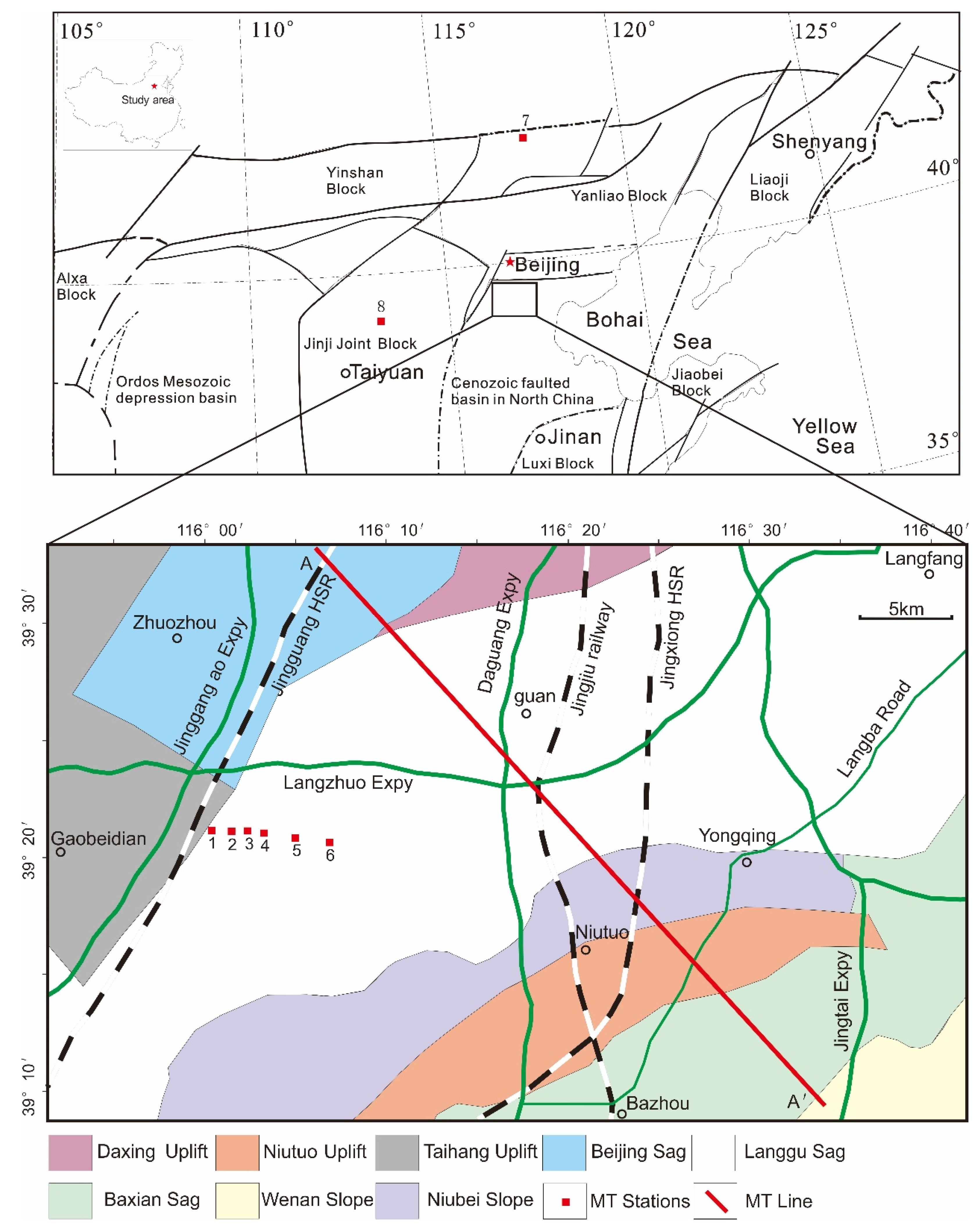
The experimental site is located in the north-central Jizhong depression, which is a graben basin that developed in the North China Craton from the Mesozoic to Cenozoic. The strata, moving from the lower to the upper, in the Jizhong depression include the Archaean Eonothem, Palaeoproterozoic Eonothem, Mesoproterozoic Erathem, Upper Proterozoic (including the Changcheng and Jixian systems), Paleogene System (including the Kongdian, Shahejie and Dongying formations), Neogene System (including the Guantao and Minghuazhen formations) and Quaternary System (the Pingyuan formation) [26]. The main lithologies of the Archaean and Palaeoproterozoic Eonothems are gneiss, with a resistivity of 100 Ωm, the Mesoproterozoic Erathem and Upper Proterozoic are carbonates, with a resistivity of 517 Ωm, the Paleogene and Neogene Systems are mudstones and sandstones, with a resistivity between 3 and 9 Ωm, and the Quaternary System includes gravels, sandstones and clays, with a resistivity of 20 Ωm [27,28].

We chose the Beijing–Guangzhou HSR (BGHSR) as the interference source for this experiment. BGHSR runs through the entire Jizhong depression, connecting Beijing and Guangzhou with a total length of 2298 km and an operating speed of 300 km per hour. There are nearly 200 trains that operate every day from 6 o’clock to 24 o’clock local time. A train passes by every few minutes. Its traction power supply system uses 25 kV, 50 Hz single-phase alternating current (AC) to provide electric energy to the train. The basic principle is that the traction substation changes the high voltage of the grid into 25 kV AC in the contact network. The electric locomotive receives current through the sliding contact of the pantograph–catenary system, flows into the rail through the high-voltage side of the vehicle-mounted traction transformer, and then returns to the traction substation from the rail to form the current loop [29]. The instantaneous value of the traction current is close to 1000 A, which greatly increases the rail current. Ideally, the rail current will return to the traction substation through the rail. However, rail aging causes leakage onto the ground and generates strong electromagnetic noise signals [11,23].

In the experiment, MT data were collected at locations situated 500 m, 1 km, 1.5 km, 2 km, 3 km and 5 km from the BGHSR near Sanlipu Village, Gaobeidian City, Hebei Province (stations 1, 2, 3, 4, 5 and 6). Then, at different distances and in different directions and geological conditions, we set up two remote reference stations (stations 7 and 8) at places where human interference is less significant and acquired data simultaneously (Figure 1). The distances between stations 1 and 7 and stations 1 and 8 were 280 km and 200 km, respectively.

The instrument used was a MTU-5A magnetotelluric acquisition system produced by the Canada Phoenix Company. A nonpolarized electrode was used to receive the electric field signal, and an inductive magnetic sensor MTC-50 was used to receive the magnetic field signal. Each station is arranged in a north–south layout for five-component acquisition. The north and the east correspond to the x and y directions, respectively, and z is perpendicular to the ground (Ex and Ey are electrical fields, and Hx, Hy and Hz are magnetic fields). The acquisition time was approximately 22 h.

3. Characteristics of HSR Noise

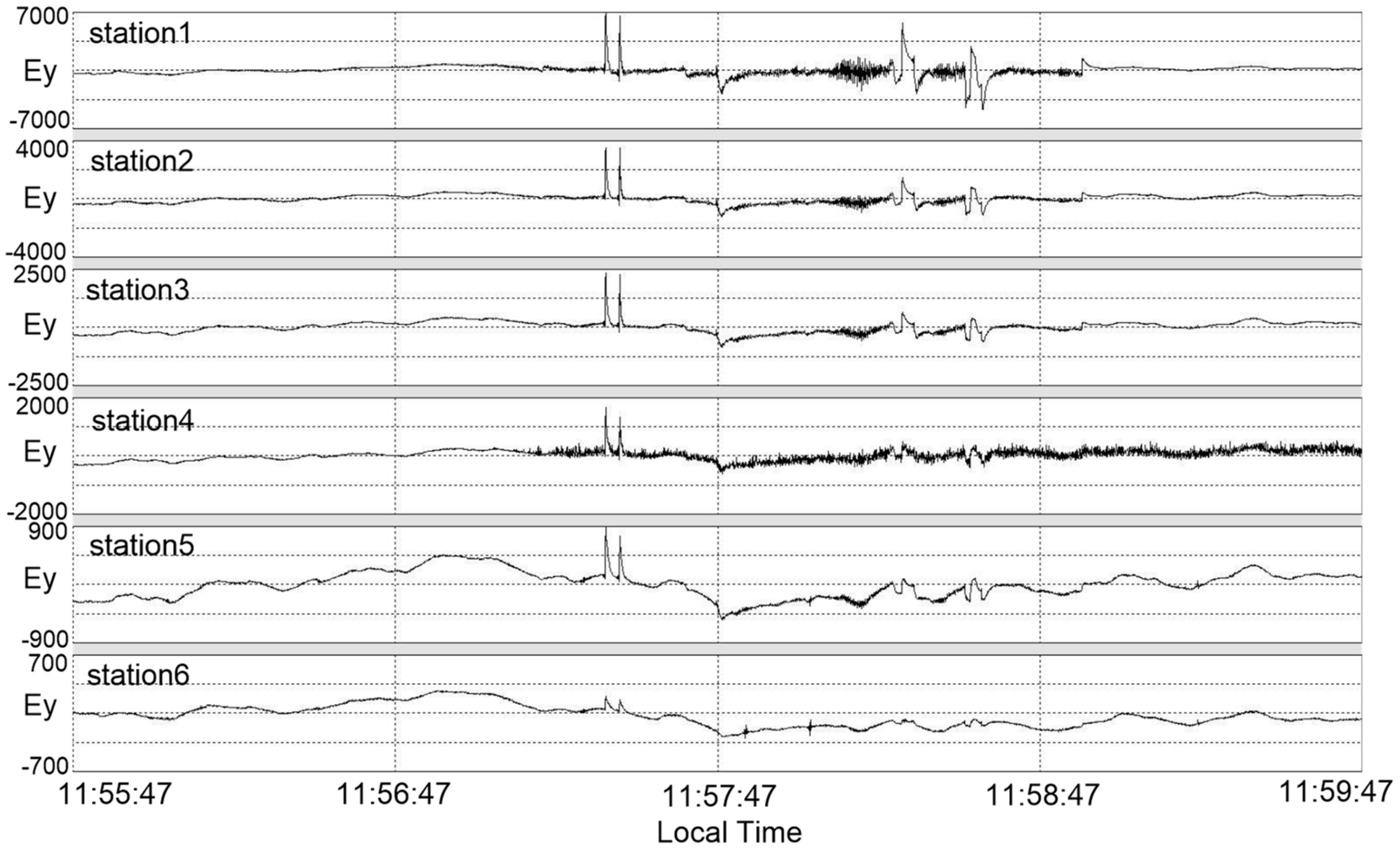
Figure 2 shows the time series of the Ey components collected by stations 1–6 at around 12 noon on 19 April 2019, local time. In the time series for the distance of 0.5 km to 5 km from the railway line, we can see impulse, charging–discharging, and triangular-wave noise. The curve jump is obvious, and its amplitude is several times or several orders of magnitude that of the natural field signals. Such noises will cause an incorrect estimation of the transfer function. As the distance increases, the noise amplitude gradually decreases, but there are still noise signals at 5 km. 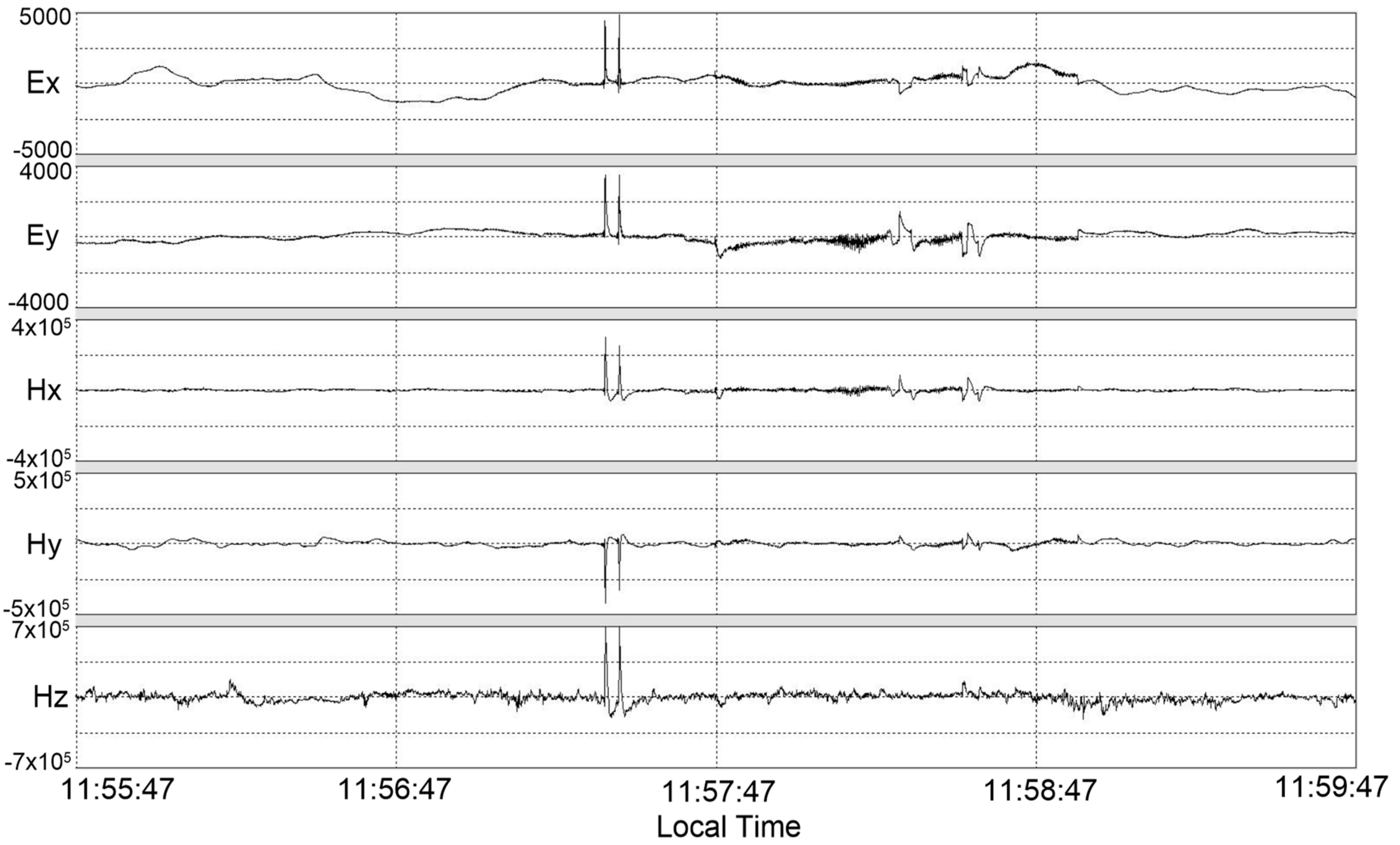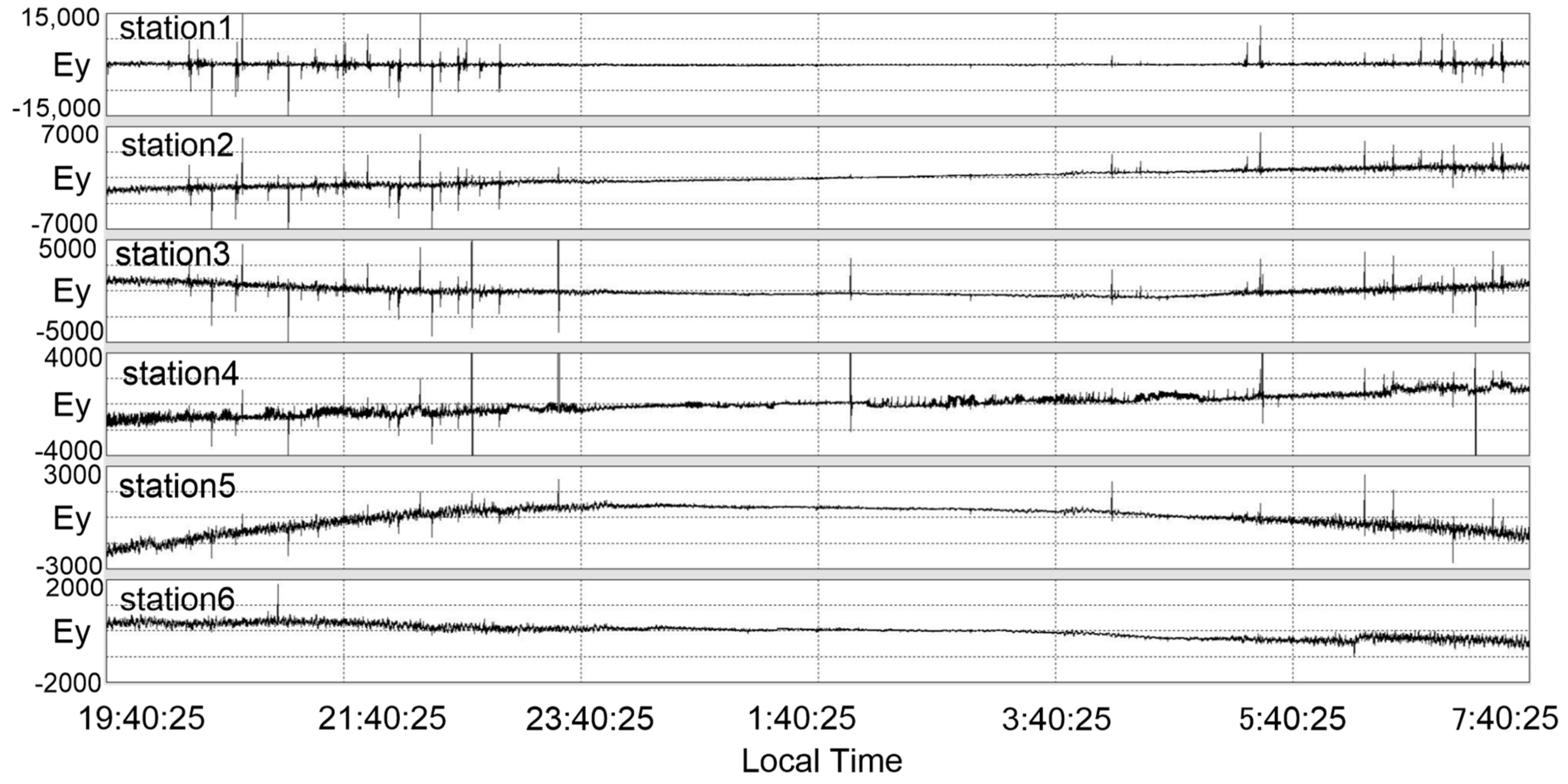Figure 3 illustrates the five components collected by station 2 at around 12 noon on 19 April 2019, local time. The HSR noise has almost the same effect on all the components. The 12 h time series (Figure 4) recorded by station 2 from 19 to 20 April 2019, local time, shows that there are almost no impulse, charging–discharging, or triangular-wave signals from 0 am to 6 am, and the amplitude is several times or several orders of magnitude smaller than that of the HSR operation period at noon. This is because various equipment of the HSR is being overhauled and trains are not running during this time. Therefore, it is better to conduct measurements at night so as to avoid HSR noise.

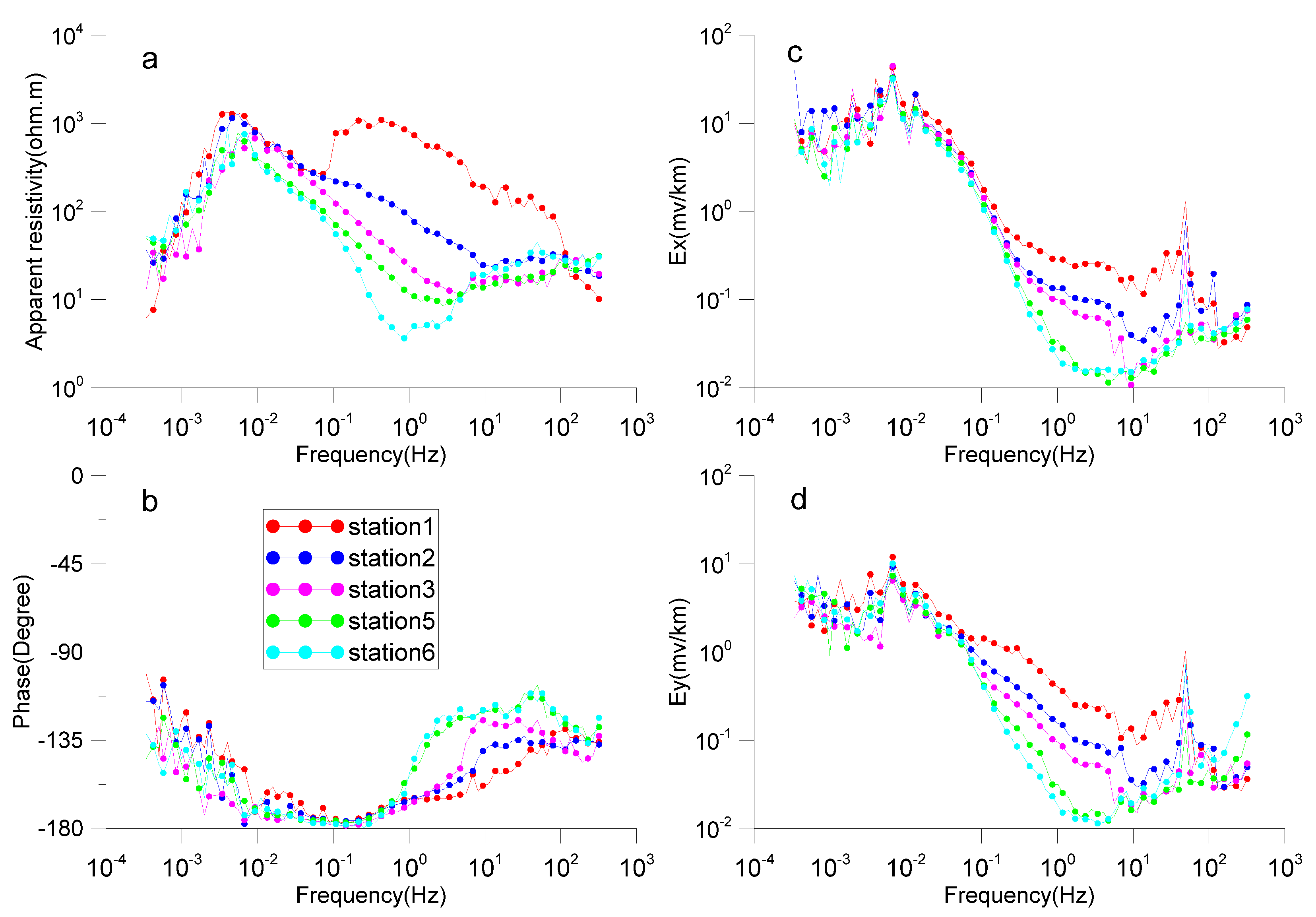
Figure 5 shows the frequency domain curves of different distances from the BGHSR. Figure 5a,b shows the apparent resistivity and phase in the y–x direction. It can be seen that the curve of station 1 is distorted from 100 Hz. For stations 2–6, the apparent resistivity and phase curves tend to overlap in the frequency range from hundreds of Hz to 10 Hz. The apparent resistivity curve below 10 Hz first decreases and then rises at a slope of nearly 45 degrees, and the phase curve tends towards −180 degrees. These are the near-field and transition zones defined by the controlled-source audio-frequency magnetotelluric method (CSAMT) [30,31,32]. As the distance increases, the frequency entering the transition zone gradually decreases, and the curves gradually separate. The apparent resistivity in the frequency range below 0.01 Hz decreases, the phase begins to rise, and the curves gradually return to normal and tend to overlap again. Figure 5c,d shows the electric field spectra in two directions. The high-frequency and low-frequency bands tend to overlap, which indicates a normal transfer function curve. In the mid-frequency band of 10–0.01 Hz, the electric field curve in the two directions and the yx apparent resistivity curve show the same trend of change, which first decreases and then rises sharply before gradually returning to normal after 0.01 Hz. 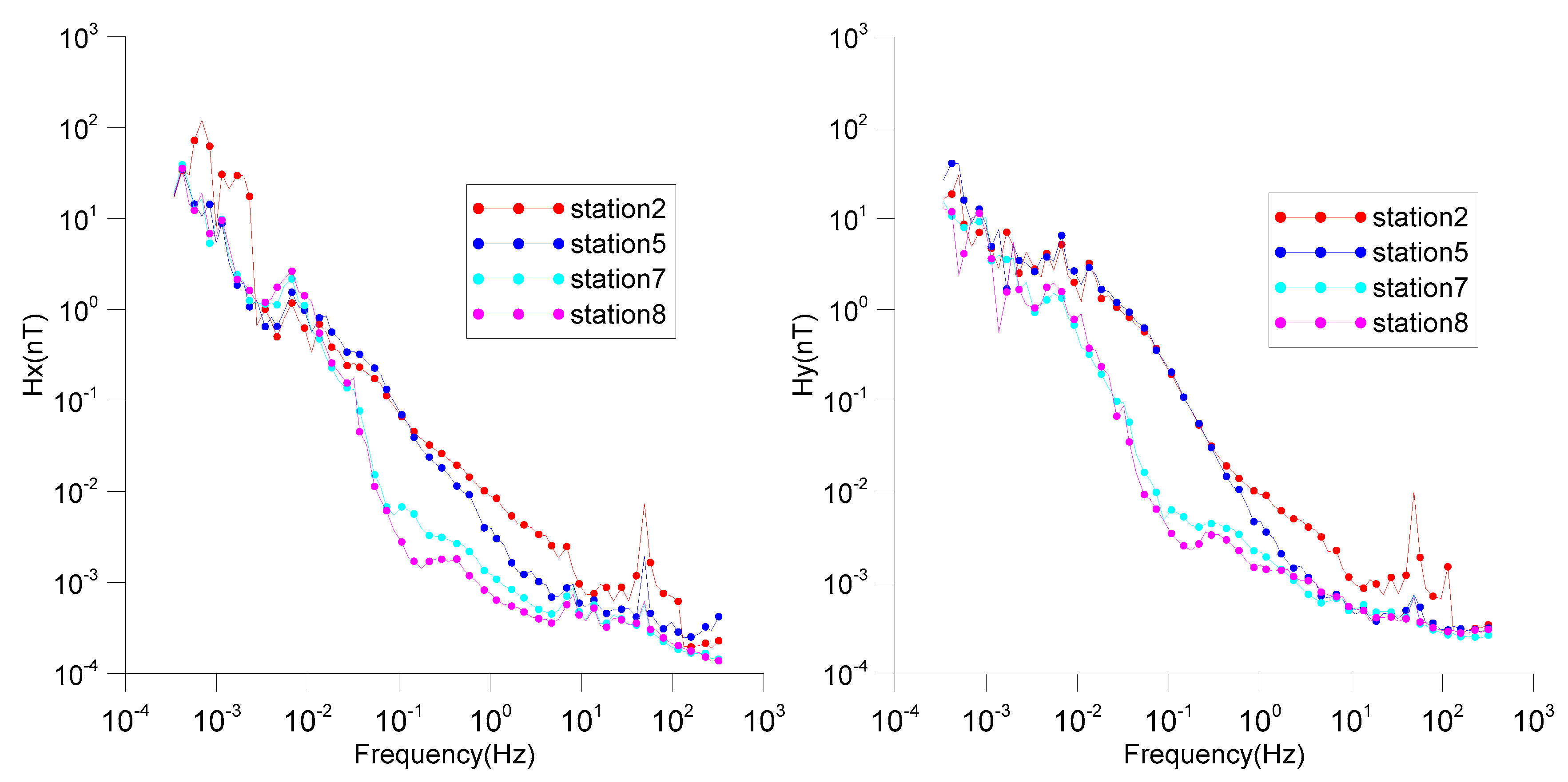Figure 6 shows the amplitude of the magnetic field. The left is Hx, and the right is Hy. Stations 2 and 5 exhibit HSR noise signals, while stations 7 and 8 are remote references and do not exhibit HSR interference signals. The amplitudes of stations 2 and 5 are very similar. Correspondingly, the amplitudes of stations 7 and 8 are very similar. The magnetic field amplitudes of stations 2 and 5 are almost an order of magnitude higher than those of stations 7 and 8 in the 10–0.01 Hz band, but these four stations are relatively close in terms of the other frequency bands. From the above analysis, it can be seen that BGHSR mainly interferes with the MT signals in the mid-frequency band of 10–0.01 Hz.

4. Effect of the Remote Reference Method (RR)

4.1. Principle of Single RR and Multiple RRs

The cross-power spectral density matrix (PSD) with RR [33], with a size of (7, 7), is shown below:

$$\left[\begin{array}{l}{\mathrm{H}}_x{\mathrm{H}}_x^{*}\\ {\mathrm{H}}_x{\mathrm{H}}_y^{*}\hspace{0.33em}\hspace{0.33em}{\mathrm{H}}_{\mathrm{y}}{\mathrm{H}}_y^{*}\\ {\mathrm{H}}_x{\mathrm{H}}_z^{*}\hspace{0.33em}\hspace{0.33em}{\mathrm{H}}_{\mathrm{y}}{\mathrm{H}}_z^{*}\hspace{0.33em}\hspace{0.33em}{\mathrm{H}}_{\mathrm{z}}{\mathrm{H}}_z^{*}\\ {\mathrm{H}}_x{\mathrm{E}}_x^{*}\hspace{0.33em}\hspace{0.33em}{\mathrm{H}}_{\mathrm{y}}{\mathrm{E}}_x^{*}\hspace{0.33em}\hspace{0.33em}{\mathrm{H}}_{\mathrm{z}}{\mathrm{E}}_x^{*}\hspace{0.33em}\hspace{0.33em}{\mathrm{E}}_{\mathrm{x}}{\mathrm{E}}_x^{*}\\ {\mathrm{H}}_x{\mathrm{E}}_y^{*}\hspace{0.33em}\hspace{0.33em}{\mathrm{H}}_{\mathrm{y}}{\mathrm{E}}_y^{*}\hspace{0.33em}\hspace{0.33em}{\mathrm{H}}_{\mathrm{z}}{\mathrm{E}}_y^{*}\hspace{0.33em}\hspace{0.33em}{\mathrm{E}}_{\mathrm{x}}{\mathrm{E}}_y^{*}\hspace{0.33em}\hspace{0.33em}\hspace{0.33em}{\mathrm{E}}_{\mathrm{y}}{\mathrm{E}}_y^{*}\\ {\mathrm{H}}_x{\mathrm{R}}_x^{*}\hspace{0.33em}\hspace{0.33em}{\mathrm{H}}_{\mathrm{y}}{\mathrm{R}}_x^{*}\hspace{0.33em}\hspace{0.33em}{\mathrm{H}}_{\mathrm{z}}{\mathrm{R}}_x^{*}\hspace{0.33em}\hspace{0.33em}{\mathrm{E}}_{\mathrm{x}}{\mathrm{R}}_x^{*}\hspace{0.33em}\hspace{0.33em}{\mathrm{E}}_{\mathrm{y}}{\mathrm{R}}_x^{*}\hspace{0.33em}\hspace{0.33em}{\mathrm{R}}_{\mathrm{x}}{\mathrm{R}}_x^{*}\\ {\mathrm{H}}_x{\mathrm{R}}_y^{*}\hspace{0.33em}\hspace{0.33em}{\mathrm{H}}_{\mathrm{y}}{\mathrm{R}}_y^{*}\hspace{0.33em}\hspace{0.33em}{\mathrm{H}}_{\mathrm{z}}{\mathrm{R}}_y^{*}\hspace{0.33em}\hspace{0.33em}{\mathrm{E}}_{\mathrm{x}}{\mathrm{R}}_y^{*}\hspace{0.33em}\hspace{0.33em}{\mathrm{E}}_{\mathrm{y}}{\mathrm{R}}_y^{*}\hspace{0.33em}\hspace{0.33em}{\mathrm{R}}_{\mathrm{x}}{\mathrm{R}}_y^{*}\hspace{0.33em}\hspace{0.33em}{\mathrm{R}}_{\mathrm{y}}{\mathrm{R}}_y^{*}\end{array}\right],$$

where the asterisk denotes the complex conjugate, and R is the magnetic or electric field of remote reference. Then, the transfer function can be written as [15,33]:

$${\mathrm{TF}=\mathrm{ER}*\mathrm{HR}}^{-1},$$

where $\mathrm{TF}=\left[\begin{array}{l}{T}_x\hspace{0.33em}\hspace{0.33em}\hspace{0.33em}{T}_y\\ Z_{xx}\hspace{0.33em}{Z}_{xy}\\ Z_{yx}\hspace{0.33em}{Z}_{yy}\end{array}\right]$, $\mathrm{ER}=\left[\begin{array}{l}{\mathrm{H}}_{\mathrm{z}}{\mathrm{R}}_x^{*}\hspace{0.33em}\hspace{0.33em}{\mathrm{E}}_{\mathrm{x}}{\mathrm{R}}_x^{*}\hspace{0.33em}\hspace{0.33em}{\mathrm{E}}_{\mathrm{y}}{\mathrm{R}}_x^{*}\\ {\mathrm{H}}_{\mathrm{z}}{\mathrm{R}}_y^{*}\hspace{0.33em}\hspace{0.33em}{\mathrm{E}}_{\mathrm{x}}{\mathrm{R}}_y^{*}\hspace{0.33em}\hspace{0.33em}{\mathrm{E}}_{\mathrm{y}}{\mathrm{R}}_y^{*}\end{array}\right]$, $\mathrm{HR}=\left[\begin{array}{l}{\mathrm{H}}_x{\mathrm{R}}_x^{*}\hspace{0.33em}\hspace{0.33em}{\mathrm{H}}_{\mathrm{y}}{\mathrm{R}}_x^{*}\\ {\mathrm{H}}_x{\mathrm{R}}_y^{*}\hspace{0.33em}\hspace{0.33em}{\mathrm{H}}_{\mathrm{y}}{\mathrm{R}}_y^{*}\end{array}\right]$.

This assumes that the signals of the local stations and RR are homologous and correlated, while the noise is uncorrelated. Thus, the PSD of the uncorrelated noise is close to zero, while only the correlated signals are retained in the ER and HR, playing a role in denoising.

The PSD matrix, including MRR, has a size of (5 + n * 2, 5 + n * 2), and n is the number of remote reference. Then, the transfer function can be written as [34,35]:

$$\mathrm{TF}=\left[\mathrm{ER}1\hspace{0.33em}\hspace{0.33em}\cdot \cdot \cdot \hspace{0.33em}\hspace{0.33em}\mathrm{ERn}\right]\hspace{0.33em}{\left[\begin{array}{l}\mathrm{HR}1\\ \hspace{0.33em}\cdot \cdot \cdot \\ \mathrm{HRn}\end{array}\right]}^{-1},$$

4.2. Effect of MRR

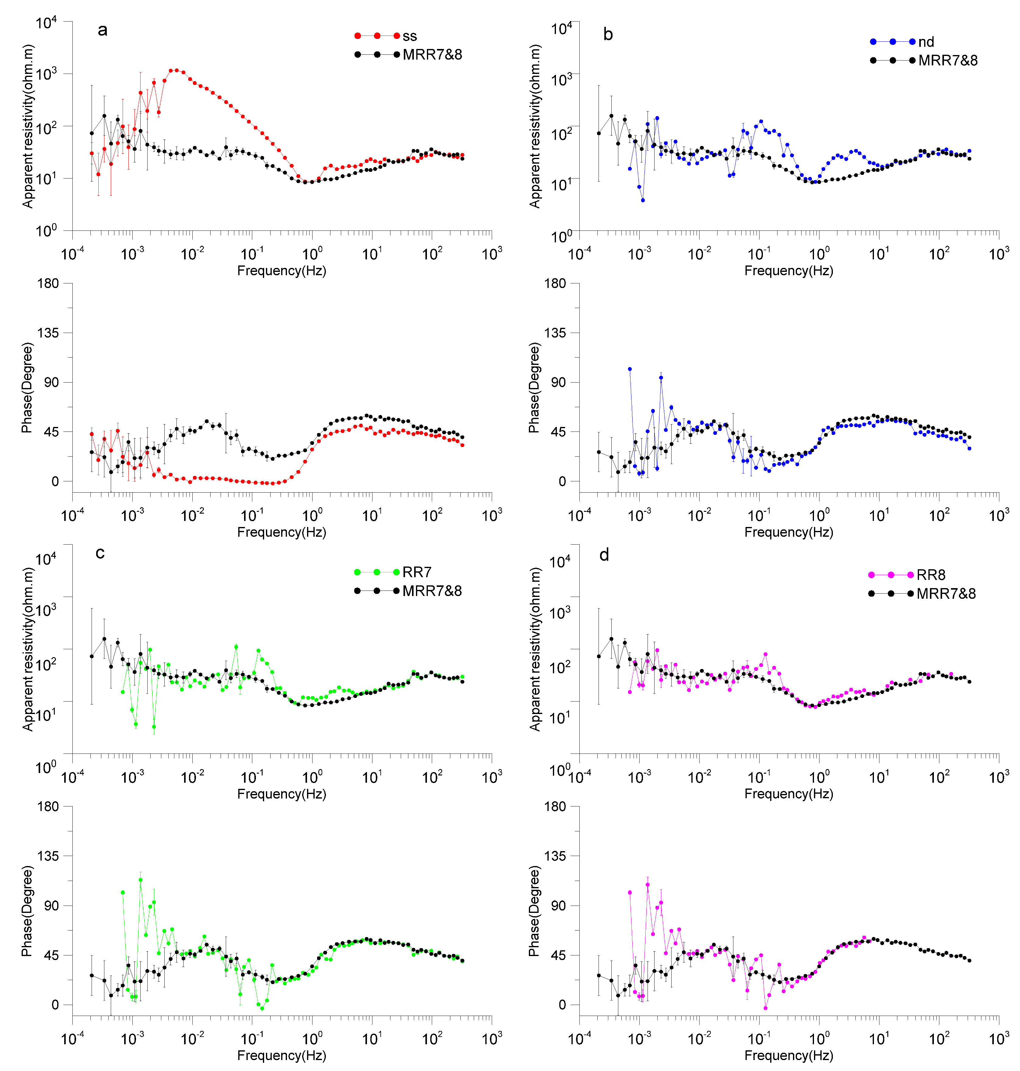
Figure 7 shows the results of station 2 (located 1 km away from the BGHSR) with respect to different RR stations. The red curves are the results of the single station (SS) without a remote reference. The apparent resistivity and phase curves are smooth and continuous. However, in the 1–0.01 Hz frequency band, the resistivity increases, with a slope of 45 degrees, and the phase tend to be −180 degrees. The near-field effect is obvious, which is inconsistent with the actual geological conditions. The blue curves are the results of nocturnal data (nd), which refer to the time period from 0 am to 6 am local time. Because there is no train running, the noise signal is weak. The near-field effect is more significantly improved, but the effect is not great in the 0.05–10 Hz frequency band. The magenta curves and green curves are the results of station 8 (RR8) and station 7 (RR7) shown as the RR. Except for the frequency band near 0.1 Hz, the near-field interference is not corrected, and the RR denoising effect of the other frequency bands is good. The black curves are the results for stations 7 and 8 shown as MRR. From the high- to low-frequency bands, there are only a few frequency jumps, but the other frequency points of the curves are convergent, the trend is obvious, and near-field interference is basically eliminated. It can be seen from this trend that the RR method greatly improves the data quality, and the MRR are more effective in removing various types of interference.

5. Results of MT Profile Experiment

In order to verify the effect of the MRR method, we arranged an MT survey line (AA’) from Matou Town, Zhuozhou City, to Liujie Township, Yongqing County, Langfang City (Figure 1). This survey line passes along the BGHSR, Beijing–Jiujiang Railway and Beijing–Xiong’an Intercity Railway and through densely populated cities such as Zhuozhou and Gu’an. Human interference of various types is particularly strong. In order to reduce the influence of cultural noise, the positions of some sites are offset at a certain distance according to the surrounding interference. The distance between the stations is approximately 1 km. There are a total of 60 stations with a total length of approximately 60 km. In this area, much exploration work has been done for many years. 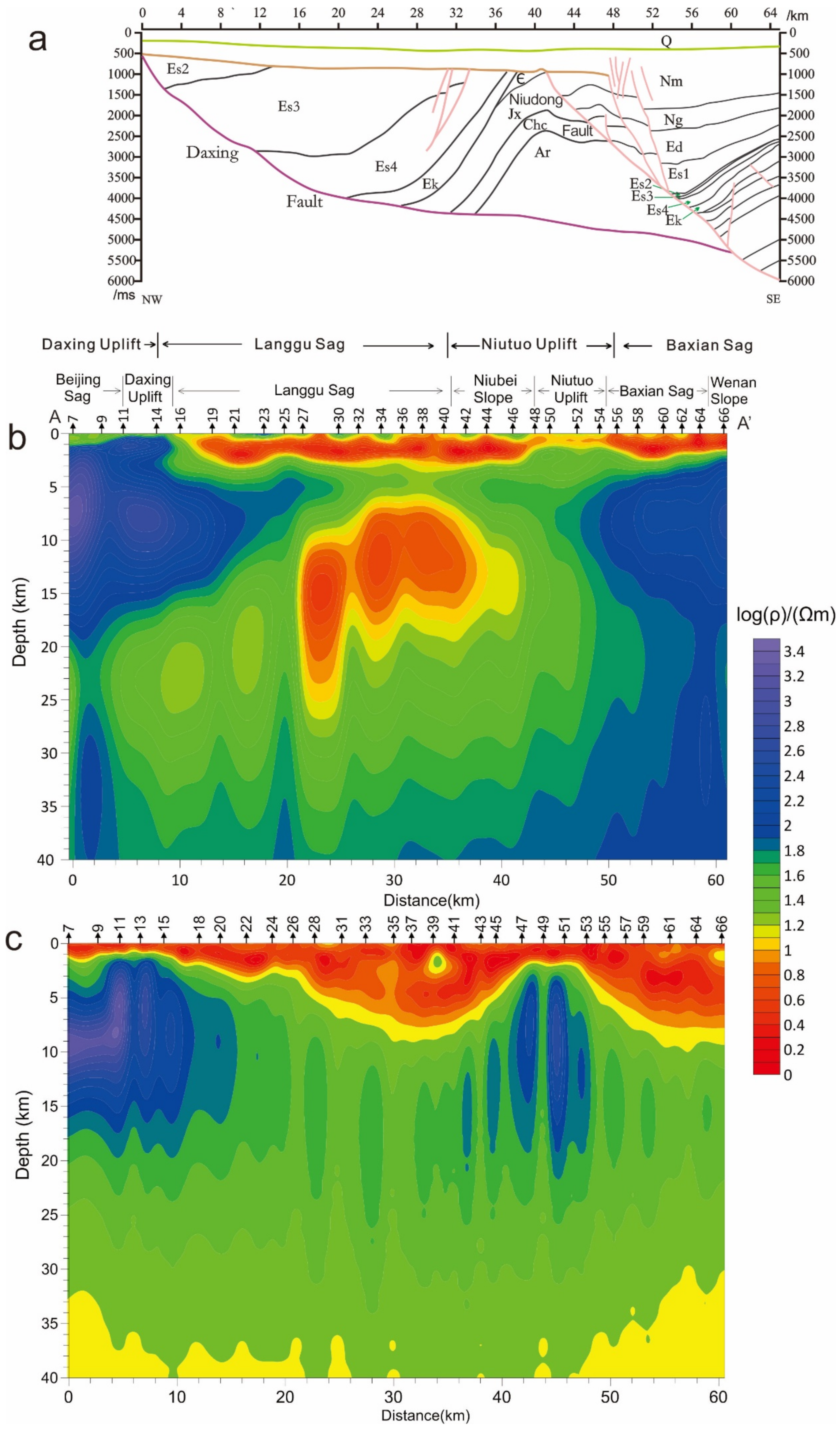Figure 8a shows a known seismic survey profile near AA’. Many deep wells have been drilled. This enables us to gain a deeper understanding of the cap layer structure and base structure of the area.

We used the impedance tensor decomposition technique for the profile data and calculated the direction of the electrical principal axis. After rotating the impedance tensor towards the geo-electric strike direction, the data of the transverse electric (TE) and traverse magnetic (TM) modes were obtained. The nonlinear conjugate gradient method (NLCG) implemented in WinGlink software was used for two-dimensional inversion [36]. The frequency range we used was 433–0.001 Hz. Frist, the poor-quality data were removed, and then the 2D inversion of the TM, TE and TM + TE modes of the apparent resistivity and impedance phases were performed [37,38]. The initial model was constructed with a uniform half-space of 100 Ωm. The data were inverted with the regularization parameter τ = 10. The inversion results of the three modes were analyzed by referring to the geological and geophysical information of the survey area. Finally, the TM + TE mode inversion result was selected because it was more consistent with the actual geological conditions. The inversion of the MRR data was completed with an RMS misfit of 2.34 after 99 iterations. The inversion of the SS data was completed with an RMS misfit of 2.24 after 103 iterations. In general, a sharp change in resistivity is often a sign of fracture or lithologic interface, where a slow change corresponds to a stable and uniform electrical layer. Therefore, the image of the contoured resistivity section can reflect the distribution law of the resistivity of the underground half-space medium along the survey line, that is, the electrical structure model of the profile. Figure 8b is a two-dimensional inversion section based on data with MRR, which clearly shows the lithologic units. From west to east, it corresponds to the Beijing sag, Daxing uplift, Langgu sag, Niutuo uplift and Baxian sag.

The upper part of the section, where the resistivity value is very low and uniform, is exactly the Langgu and Baxian sag, where the Cenozoic deposits are very thick. The resistivity value also reflects the shallow-buried Daxing and Niutuo uplifts.

Figure 8a is a seismic section very close to AA’ [26,39], and the average wave speed is approximately 3000 m/s. It shows that the reflected underground structure is almost the same as that in Figure 8b. Figure 8b shows the inversion result of the data with MRR (7 and 8). The depth of the bedrock interface in the figure and the seismic profile are basically the same. Figure 8c shows the inversion result of the data for a single station, which reflects the tectonic units to a certain extent, but the horizontal partition is not obvious, and the vertical stratification is not clear. The low-resistivity layer in the crust at a depth of more than 10 km underground is not reflected [40]. The bedrock interface is deeper [41].

6. Discussion and Conclusions

BGHSR noise has a fixed shape in the time domain waveform, and the amplitude is very large, which can be observed from the electromagnetic field. The interfering signals between each station or between all components of the same station are highly correlated, but the polarization directions are different. These features can provide a basis for removing the noise of HSR.

From the definition of CSAMT, the high-frequency band of the HSR noise signals above 10 Hz is in the far field, which approaches the MT assumption of quasi-homogeneous fields and is included as part of the MT signals. Therefore, the signals in this frequency band are enhanced [23]. The mid-frequency band (10–0.01 Hz) enters the transition zone and near zone, causing the field source effect. There is no HSR noise in the low-frequency band, and the MT signals are restored to quasi-homogeneous fields.

When station 7 or station 8 is used as an RR, the near-field interference is not effectively removed. In the frequency band near 0.1 Hz, the so-called “dead band” [42,43], it is likely that the natural field signal in this frequency band will be weak, and the denoising ability of RR is also reduced, resulting in unreliable data.

We analyzed the noise signals of the BGHSR in the time domain and frequency domain and found that they are mainly impulse, charging–discharging and triangular-wave noises. The distance of the interference exceeds 5 km, and the interference frequency band is mainly in the range of 10–0.01 Hz.

The MRR method [34,35] is better than the single-RR method [15,33], since it can remove human interference more effectively and obtain high-quality MT data.

Although the MRR method has an ideal effect in removing interference, it is not a panacea. When one data point in the remote reference data is not good or has less coherence with the station data, the result may be inferior to the single remote reference. In the future, we will consider how to select remote reference data of different frequencies, and the remote reference data frequency bands with poor denoising effects will not be involved in the calculation so as to improve the noise removal effect. The farther away the noise sources are, the smaller their impact on the data is. Therefore, it is also very important to arrange instruments in the field as far away as possible so as to avoid noise sources.

References

- Gurk, M.; Bosch, F.P.; Tougiannidis, N. Electric field variations measured continuously in free air over a conductive thin zone in the tilted lias-epsilon black shales near Osnabrück, northwest Germany. J. Appl. Geophys. 2013, 91, 21–30. [Google Scholar] [CrossRef]
- Wannamaker, P.E.; Doerner, W.M. Crustal structure of the RubyMountains and southern Carlin Trend region, Nevada, frommagnetotelluric data. Ore Geol. Rev. 2002, 21, 185–210. [Google Scholar] [CrossRef]
- Meng, Y.S.; Chen, X.Q.; Wang, W.G.; Li, R.H.; Wang, G. Geophysical Implications for Prospective Prediction of Copper Polymetallic Ore Bodies: Northern Margin of Alxa Block, China. Minerals 2022, 12, 653. [Google Scholar] [CrossRef]
- Ádám, A.; Novák, A.; Szarka, L.; Wesztergom, V. The magnetotelluric (MT) investigation of the Diósjenő dislocation belt. Acta Geod. Et Geophys. 2003, 38, 305–326. [Google Scholar] [CrossRef]
- Cagniard, L. Basic theory of the magnetotelluric method of geophysical prospecting. Geophysics 1953, 18, 605–635. [Google Scholar] [CrossRef]
- Mehanee, S.; Zhdanov, M. A quasi-analytical boundary condition for three-dimensional finite difference electromagnetic modeling. Radio Sci. 2004, 39, RS6014. [Google Scholar] [CrossRef] [Green Version]
- Feucht, D.W.; Sheehan, A.F.; Bedrosian, P.A. Magnetotelluric Imaging of Lower Crustal Melt and Lithospheric Hydration in the Rocky Mountain Front Transition Zone, Colorado, USA. J. Geophys. Res. Solid Earth 2017, 122, 9489–9510. [Google Scholar] [CrossRef]
- Hanekop, O.; Simpson, F. Error propagation in electromagnetic transfer functions: What role for the magnetotelluric method in detecting earthquake precursors. Geophys. J. Int. 2006, 165, 763–774. [Google Scholar] [CrossRef]
- Maithya, J.; Fujimitsu, Y. Analysis and interpretation of magnetotelluric data in characterization of geothermal resource in Eburru geothermal field, Kenya. Geothermics 2019, 81, 12–31. [Google Scholar] [CrossRef]
- Zhang, L.L.; Zhao, C.J.; Yu, P.; Xiang, Y.; Peng, X.C.; Koyama, T.; Yang, W.C. The electrical conductivity structure of the Tarim basin in NW China as revealed by three-dimensional magnetotelluric inversion. J. Asian Earth Sci. 2020, 187, 104093. [Google Scholar] [CrossRef]
- Padilha, A.L.; Vitorello, I.; Brito, P.M.A. Magnetotelluric soundings across the Taubat Basin, Southeast Brazil, Earth. Planets Space 2002, 54, 617–627. [Google Scholar] [CrossRef] [Green Version]
- Szarka, L. Geophysical aspects of manmade electromagnetic noise in the earth—A review. Surv. Geophys. 1988, 9, 287–318. [Google Scholar] [CrossRef]
- Takahashi, I.; Hattori, K.; Harada, M.; Yoshino, C. Anomalous geoelectrical and geomagnetic signals observed at Southern Boso Peninsula, Japan. Ann. Geophys. 2007, 50, 123–135. [Google Scholar] [CrossRef]
- Larsen, J.C.; Mackie, R.L.; Manzella, A.; Fiordelisi, A.; Rievenj, S. Robust smooth magnetotelluric transfer functions. Geophys. J. Int. 1996, 124, 801–819. [Google Scholar] [CrossRef]
- Goubau, W.; Gamble, T.; Clarke, J. Magnetotelluric data analysis: Removal of bias. Geophysics 1978, 43, 1157–1166. [Google Scholar] [CrossRef]
- Gamble, T.D.; Goubau, W.M.; Clarke, J. Magnetotellurics with a remote magnetic reference. Geophysics 1979, 44, 53–68. [Google Scholar] [CrossRef] [Green Version]
- Egbert, G.D.; Booker, J.R. Robust estimation of geomagnetic transfer functions. Geophys. J. Int. 1986, 87, 173–194. [Google Scholar] [CrossRef] [Green Version]
- Tang, J.T.; Cai, J.H.; Ren, Z.Y.; Hua, X.R. Hilbert-Huang transform and time-frequency analysis of magnetotelluric signal. J. Cent. South Univ. (Sci. Technol.) 2009, 5, 1399–1405. [Google Scholar]
- Trad, D.O.; Travassos, J.M. Wavelet filtering of magnetotelluric data. Geophysics 2000, 65, 482–491. [Google Scholar] [CrossRef]
- Tang, J.T.; Li, J.; Xiao, X.; Zhang, L.C.; Lü, Q.T. Mathematical morphology filtering and noise suppression of magnetotelluric sounding data. Chin. J. Geophys. 2012, 55, 1784–1793. [Google Scholar]
- Zhou, Y.Y.; Chang, Y.; Chen, H. Application of reference based blind source separation method in the reduction of near field noise of geomagnetic measurements. Chin. J. Geophys. 2019, 62, 572–586. [Google Scholar]
- Bhattacharya, B.B.; Shalivahan. Application of robust processing of magnetotelluric data using single and remote reference sites. Curr. Sci. 1999, 76, 1108–1113. [Google Scholar]
- Oettinger, G.; Haak, V.; Larsen, J.C. Noise reduction in magnetotelluric time-series with a new signal-noise separation method and its application to a field experiment in the Saxonian Granulite Massif. Geophys. J. Int. 2001, 146, 659–669. [Google Scholar] [CrossRef] [Green Version]
- Shalivahan; Bhattacharya, B.B. How remote can the far remote reference site for magnetotelluric measurements be? J. Geophys. Res. Solid Earth 2002, 107, 2105. [Google Scholar] [CrossRef]
- Wang, H.; Chen, J.L.; Teng, X.Z. Source effect on magnetotelluric data due to mining area and its suppression. Prog. Geophys. 2016, 31, 1358–1366. (In Chinese) [Google Scholar]
- He, D.F.; Cui, Y.Q.; Zhang, Y.Y.; Shan, S.Q.; Xiao, Y.; Zhang, C.B.; Zhou, C.A.; Gao, Y. Structural genetic types of paleoburied hill in Jizhong depression, Bohai Bay Basin. Acta Petrol. Sin. 2017, 33, 1338–1356. [Google Scholar]
- Miao, Q.Z.; Wang, G.L.; Xing, L.X.; Zhang, W.; Zhou, X.N.; Wang, W.Q. Study on application of deep thermal reservoir by using geophysical and geochemical methods in the Jizhong depression zone. Acta Geol. Sin. 2020, 94, 2147–2156. [Google Scholar]
- Shi, Z.; Zhang, H.; Duan, T.; Zhang, P. Investigation of oil and gas reservoir in Jizhong depression based on time-frequency electromagnetic method. Glob. Geol. 2018, 37, 585–594. [Google Scholar]
- Lin, G.S.; Gao, S.B. Selective-tripping scheme for power supply arm on high-speed railway based on correlation analysis between feeder current fault components in multisite. IEEJ Trans. Electr. Electron. Eng. 2019, 14, 773–779. [Google Scholar] [CrossRef]
- Goldstein, M.A.; Strangway, D.W. Audio-frequency magnetotellurics with a grounded electric dipole source. Geophysics 1975, 40, 669–683. [Google Scholar] [CrossRef]
- Wang, G.; Lei, D.; Zhang, Z.Y.; Hu, X.Y.; Li, Y.B.; Wang, D.Y.; Zhu, W. Tensor CSAMT and AMT Studies of the Xiarihamu Ni-Cu Sulfide Deposit in Qinghai, China. J. Appl. Geophys. 2018, 159, 795–802. [Google Scholar] [CrossRef]
- Zonge, K.L.; Hughes, L.J. Controlled Source Audio-Frequency Magnetotellurics. In Electromagnetic Methods in Applied Geophysics—Applications—Part A and Part B; SEG (Society of Exploration Geophysicists): Houston, TX, USA, 1991; Volume 2, pp. 713–810. [Google Scholar]
- Gamble, T.D.; Goubau, W.M.; Clarke, J. Error analysis for remote reference Magnetotellurics. Geophysics 1979, 44, 959–968. [Google Scholar] [CrossRef]
- Chave, A.D.; Thomson, D.J. Bounded influence magnetotelluric response function estimation. Geophys. J. Int. 2004, 157, 988–1006. [Google Scholar] [CrossRef]
- Smaï, F.; Wawrzyniak, P. Razorback, an open source Python library for robust processing of magnetotelluric data. Front. Earth Sci. 2020, 8, 296. [Google Scholar] [CrossRef]
- Rodi, W.; Mackie, R.L. Nonlinear conjugate gradients algorithm for 2-D magnetotelluric inversion. Geophysics 2001, 66, 174–187. [Google Scholar] [CrossRef]
- Mehanee, S.; Zhdanov, M. Two-dimensional magnetotelluric inversion of blocky geoelectrical structures. J. Geophys. Res. Solid Earth 2002, 107, EPM 2-1–EPM 2-11. [Google Scholar] [CrossRef]
- Mehanee, S.; Golubev, N.; Zhdanov, M. Weighted regularized inversion of magnetotelluric data. In Expanded Abstract Presented at the 68th International and Meeting; Society of Exploration Geophysicists: New Orleans, LA, USA, 1998. [Google Scholar]
- He, D.F.; Cui, Y.Q.; Shan, S.Q.; Xiao, Y.; Zhang, Y.Y.; Zhang, C.B. Characteristics of geologic framework of buried-hill in Jizhong depression, Bohai Bay Basin. Chin. J. Geol. 2018, 53, 1–24. [Google Scholar]
- Zhan, Y.; Zhao, G.Z.; Wang, L.F.; Wang, J.J.; Xiao, Q.B. Deep structure in shijiazhuang and the vicinity by magnetotellurics. Seismol. Geol. 2011, 33, 913–927. [Google Scholar]
- He, D.F.; Shan, S.Q.; Zhang, Y.Y.; Lu, R.Q.; Zhang, R.F.; Cui, Y.Q. 3-D geologic architecture of Xiong’an New Area: Constraints from seismic reflection data. Sci. China Earth Sci. 2018, 61, 1007–1022. [Google Scholar] [CrossRef]
- Santarato, I. On the interference of man-made EM fields in the magnetotelluric ‘dead band’. Geophys. Prospect. 1999, 47, 707–719. [Google Scholar]
- Xavier, G.; Alan, G.J. Robust processing of magnetotelluric data in the AMT dead band using the continuous wavelet transform. Geophysics 2008, 73, F223–F234. [Google Scholar]