Article

Predictive Modeling and Analysis of Material Removal Characteristics for Robotic Belt Grinding of Complex Blade

1
College of Mechanical Engineering, Zhejiang University of Technology, Liuxia Street, Xihu District, Hangzhou 310023, China
2
State Key Laboratory of Fluid Power Transmission and Control, Zhejiang University, Hangzhou 310027, China
3
R&D Engineering Department, Wahaha Intelligent Robotics, Xiaoshan Economic and Technological Development Zone, Xiaoshan District, Hangzhou 311231, China
*
Author to whom correspondence should be addressed.
Appl. Sci. 2023, 13(7), 4248; https://doi.org/10.3390/app13074248
Submission received: 1 March 2023 / Revised: 21 March 2023 / Accepted: 22 March 2023 / Published: 27 March 2023

Abstract

:
High-performance grinding has been converted from traditional manual grinding to robotic grinding over recent years. Accurate material removal is challenging for workpieces with complex profiles. Over recent years, digital processing of grinding has shown its great potential in the optimization of manufacturing processes and operational efficiency. Thus, quantification of the material removal process is an inevitable trend. This research establishes a three-dimensional model of the grinding workstation and designs the blade back arc grinding trajectory. A prediction model of the blade material removal depth (MRD) is established, based on the Adaptive Neuro-Fuzzy Inference System (ANFIS). Experiments were carried out using the Taguchi method to investigate how certain elements might affect the outcomes. An Analysis of Variance (ANOVA) was used to study the effect of abrasive belt grinding characteristics on blade material removal. The mean absolute percent error ( M A P E ) of the established ANFIS model, after training and testing, was 3.976%, demonstrating superior performance to the reported findings, which range from 4.373% to 7.960%. ANFIS exhibited superior outcomes, when compared to other prediction models, such as random forest (RF), artificial neural network (ANN), and support vector regression (SVR). This work can provide some sound guidance for high-precision prediction of material removal amounts from surface grinding of steam turbine blades.

1. Introduction

As the essential component of steam turbines, steam turbine blades must be constructed with extreme precision to withstand demanding working conditions. However, when traditional processing methods are used by workers to grind the blade, the grinding precision is solely dependent on the worker’s subjective perception [1,2]. Due to the inadequate grinding environment, manual grinding is ineffective, unable to produce accurate material removal and unhealthy for workers. Instead, robotic grinding has emerged as a competitive option to hand grinding of workpieces with complex surfaces, because of its adaptability, intelligence and lower cost [3,4,5]. Furthermore, the enormous curve of the blade profile and the intricate microscopic material removal mechanism make it challenging to quantify the quantity of blade grinding removal under certain grinding conditions [6]. Therefore, it is especially important to develop a model that can predict material removal correctly. Over the years, there has been considerable interest in the prediction of material removal depth (MRD) based on complicated profiles. Likewise, numerous approaches have been tested to address this bottleneck issue [7,8]. However, the majority of material removal research is primarily modeled by simulating the contact conditions between the workpiece surface and the abrasive tool. These models are prone to significant mistakes because they frequently overlook the state of the abrasive tool itself and base assumptions on ideal circumstances. In order to study the relationship between material removal depth and process parameters, Hamann [9] proposed a mathematical model:
r = C A K A k t V b V w L w F A
where C A is the grinding process constant, K A represents the resistance constant of abrasive belt grinding ability, k t is the abrasive belt wear coefficient, V b is the abrasive belt rate, V w is the feed rate, L w is the width of the grinding path, F A is the normal force between the workpiece and the grinding tool. Since Hamann’s model is only suitable for workpieces with relatively flat surfaces, it is no longer applicable to workpieces with complex profiles. A model proposed by Preston [10] for material removal depth versus pressure and relative velocity between workpiece and grinding tool is widely used in the grinding industry:
d h d t = k p P ( V s ± V w )
where k p is the Preston coefficient, P is the normal force between the workpiece and the grinding tool, V s is the grinding tool speed, V w is the workpiece feed speed, and “±” indicates the contact direction between workpiece and grinding tool. The grinding equation has a more comprehensive summary of the grinding process, but the dimensionless constant k p used in the formula can only be determined through very detailed physical experiments, which are not universal. In order to solve the problem of free-form surface material removal, Xiang Zhang et al. [3] proposed a local material removal grinding model for turbine blades. Zhang’s model is a local process model with force as the main influencing factor of final local removal, which is convenient in understanding and defining the free-form surface process model. In order to address the low grinding accuracy of complex blade profiles, Yuanjian Lv [
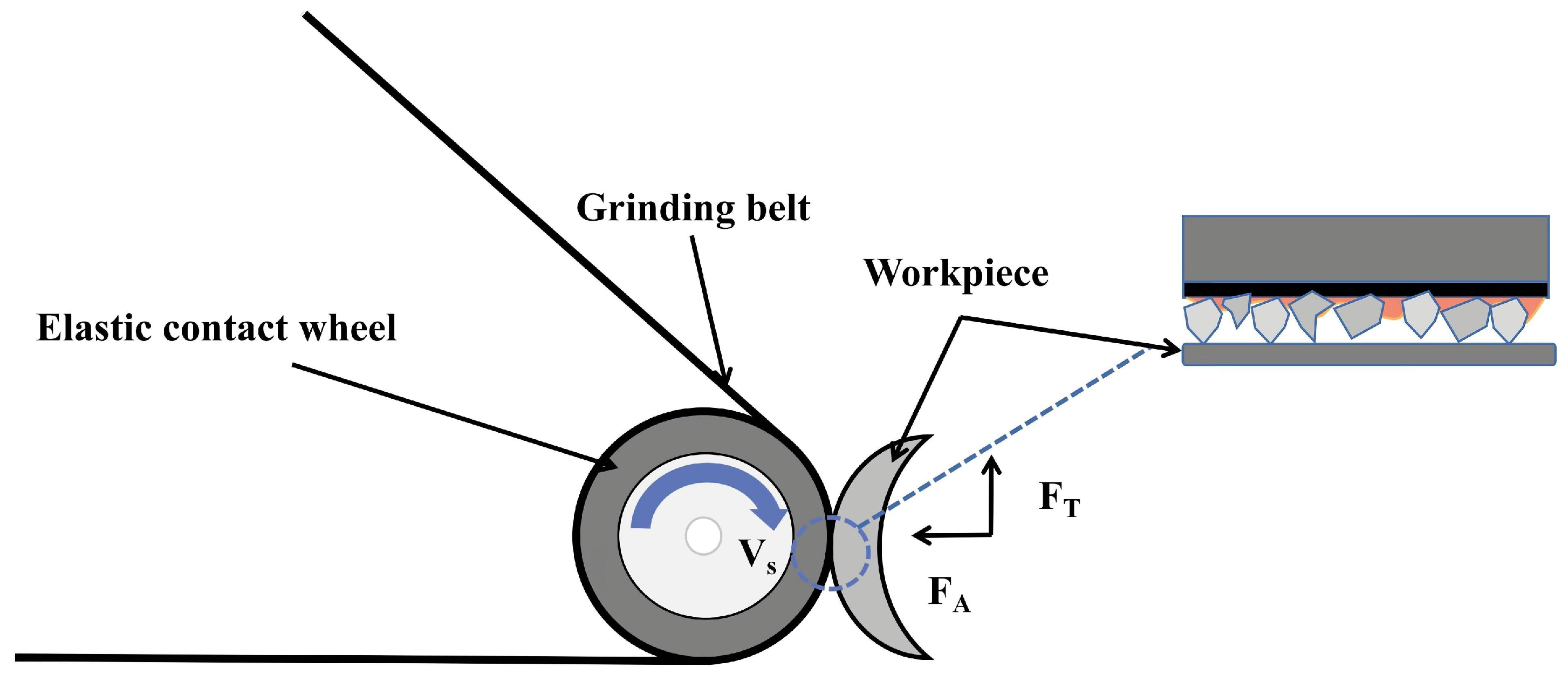
6] suggested an equal residual height technique, based on the material removal profile (MRP) model. Lv’s model designs the workpiece’s grinding path, while taking into account the contact wheel’s elastomeric deformation. Therefore, the accuracy of grinding for some blades is significantly improved. In the actual grinding process, many factors impact on the final grinding removal rate, including abrasive belt mesh number, rotational speed, and grinding force [11,12,13]. In order to achieve accurate material removal depth, these key parameters must be taken into account. In addition, the main cause of the significant discrepancy between the model calculation result and the actual one is, frequently, due to disregarding the actual grinding scenario. A large amount of experimental data is obtained from the actual grinding parameters, and this is a more appropriate method in using the nonlinear regression model over the traditional model.
Over the last few years, the application of machine learning algorithms has attracted more and more attention in the fields of manufacturing and processing [14,15]. Furthermore, future development will increasingly favor the use of big data to advance the manufacturing and processing industries. Khalick Mohammad et al. [16] proposed a polishing algorithm utilizing the composition of neural networks (NNWs) and genetic algorithms (GAs). Mohammad’s algorithm solves the problem of uneven distribution of materials removed from the surface to be polished. More specifically, the effectiveness of the algorithm is verified by polishing experiments on uneven surfaces. Kaiyuan Gao [17] proposed a machine learning and acoustic sensing approach for Inconel 718 robot belt abrasive material removal. The material removal model included a newly trained and improved K-fold-XGBoost algorithm. Data-driven models have become a hot topic in the engineering world with the emergence of machine learning and deep learning algorithms. This argument is satisfactorily made by Pandiyan [18]. This paper’s method, ANFIS, is in line with how data-driven models are applied in the engineering discipline. While other literature studies use rigid tools or flexible tools to grind flat workpieces, this study makes a unique addition by using flexible grinding tools to grind curved workpieces [19].
Support vector machine (SVM), neural network (NN), and fuzzy logic (FL) have been the three most popular learning techniques over the past 20 years. SVM, NN, and FL were the three comparison algorithms used by Kecman [20]. Wahyu Caesarendra [21] used offline machine learning to deburr vibration data using wavelet decomposition, the Welch technique, and ANFIS. They also contrasted the ANFIS classifier against the SVM classifier, neural network classifier, and both. Pandiyan [
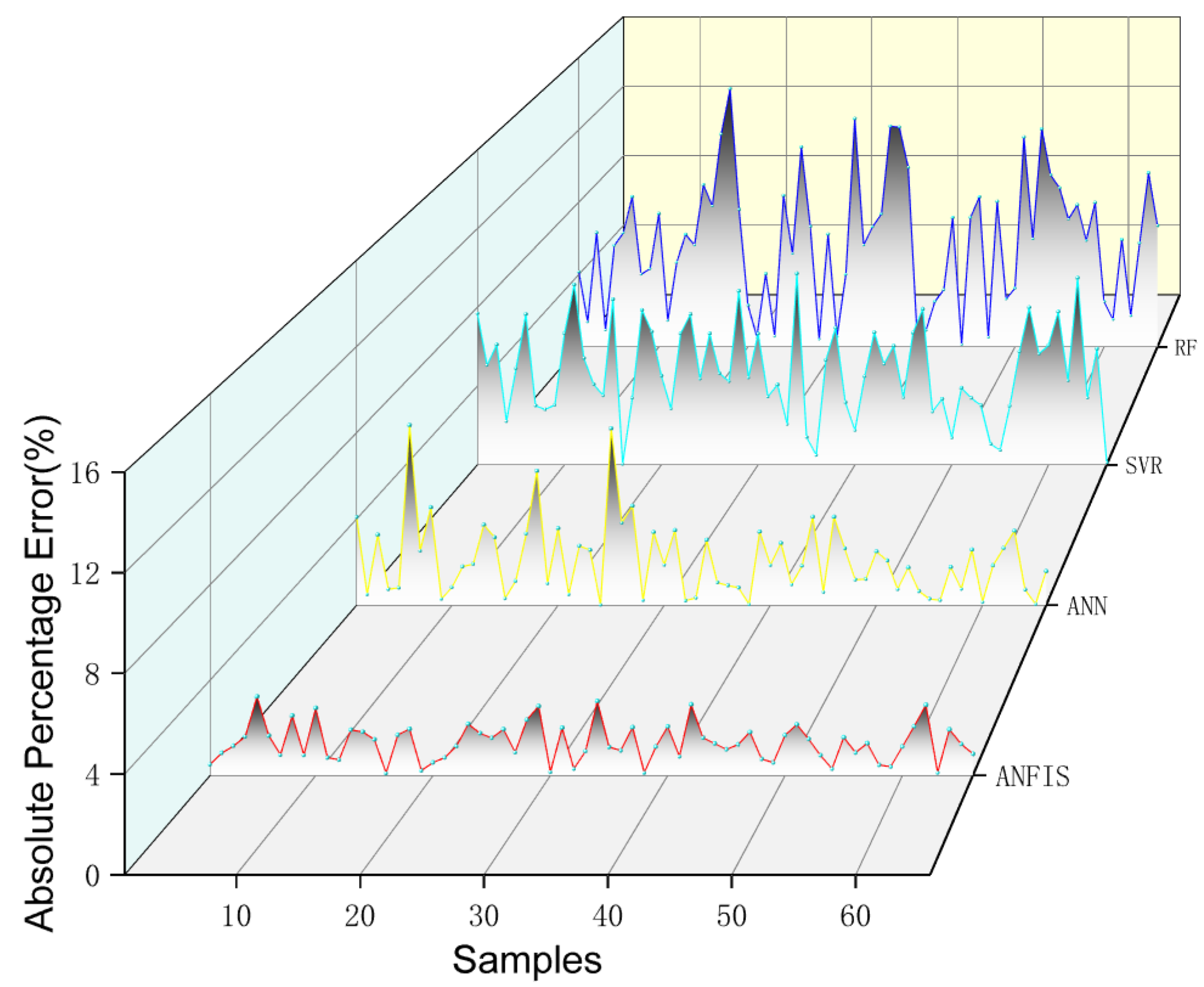
14] carried out thorough comparisons with grinding data using methods like ANFIS, Artificial Neural Networks (ANN), Support Vector Regression (SVR), Random Forest (RF), etc. Based on the research in the above literature, this paper used the data obtained from the experiments to compare and analyze the four regression algorithms (ANFIS, ANN, SVR, and RF), and this provided a scientific basis for the selection of the ANFIS method.
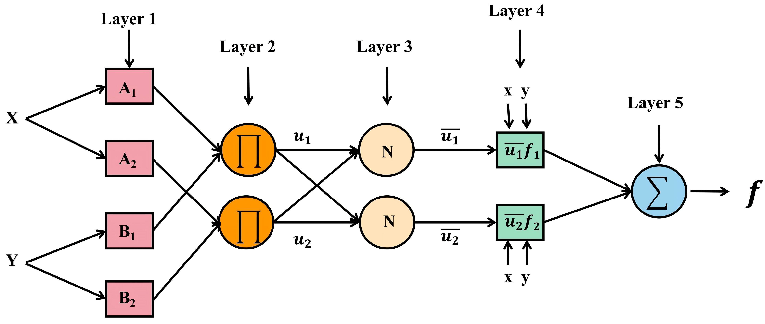
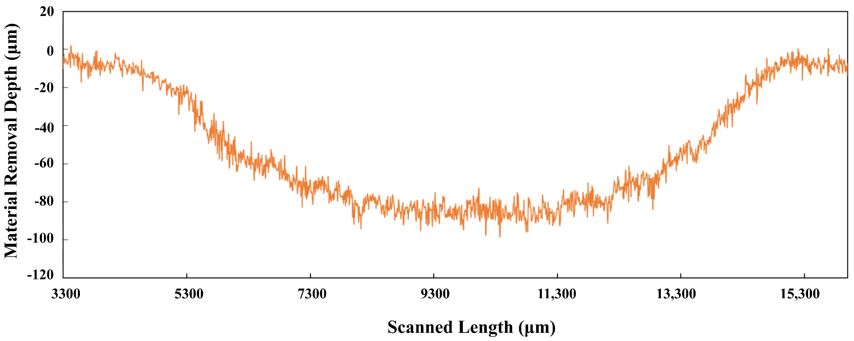
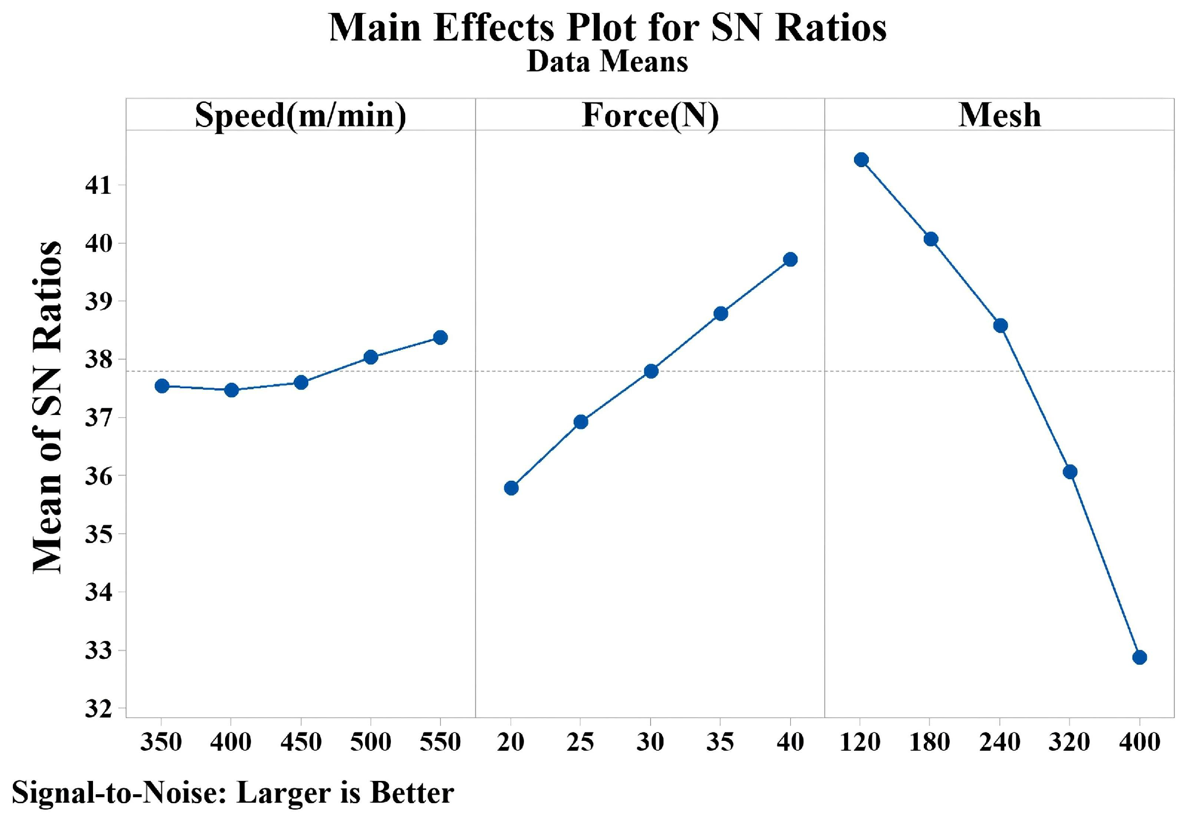
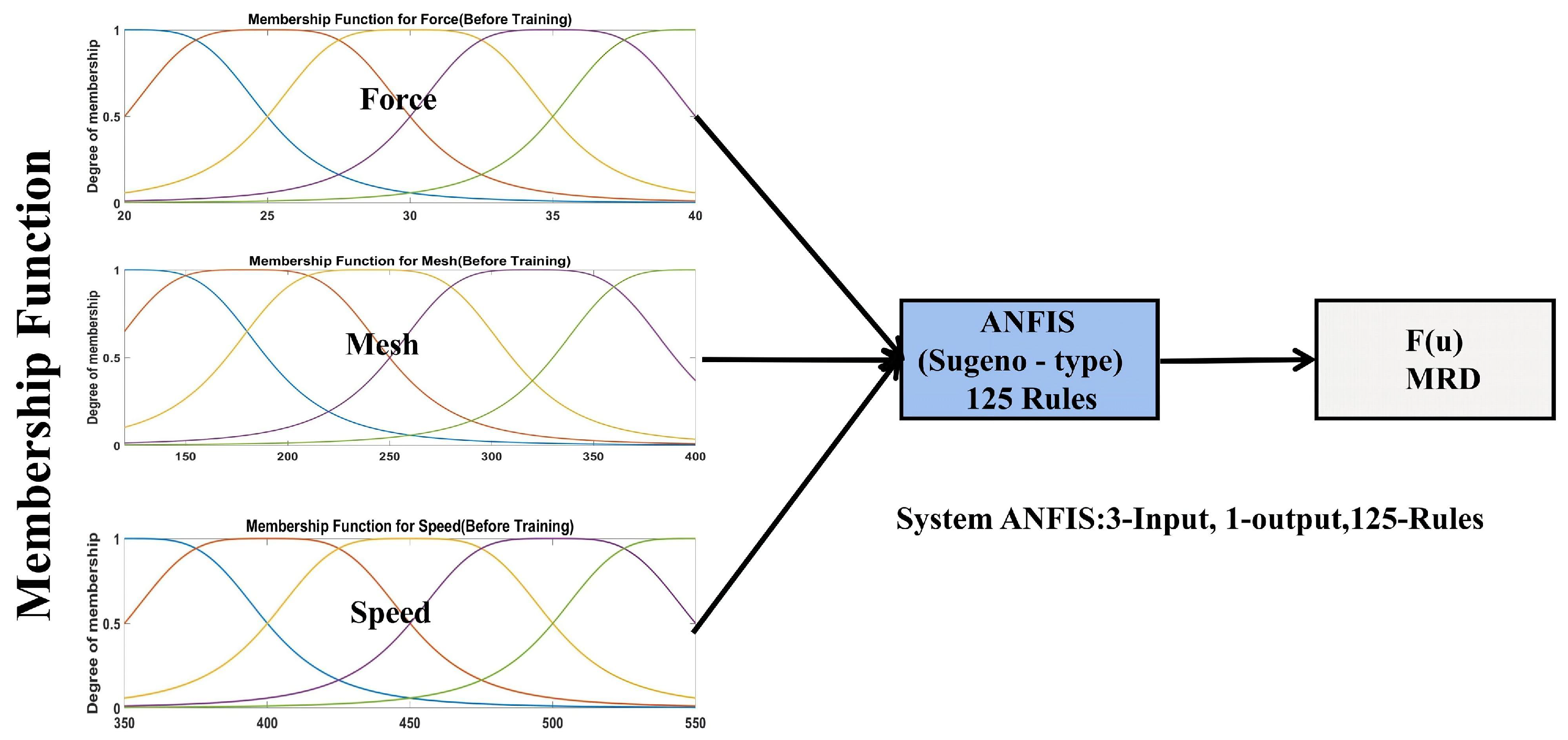
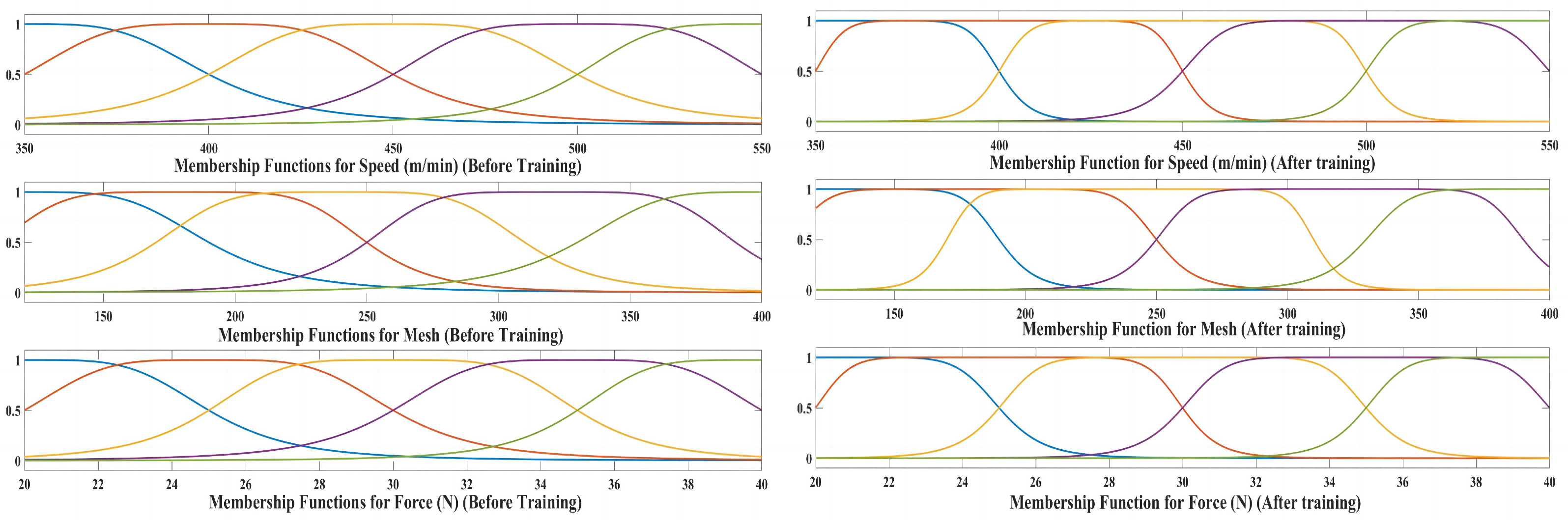
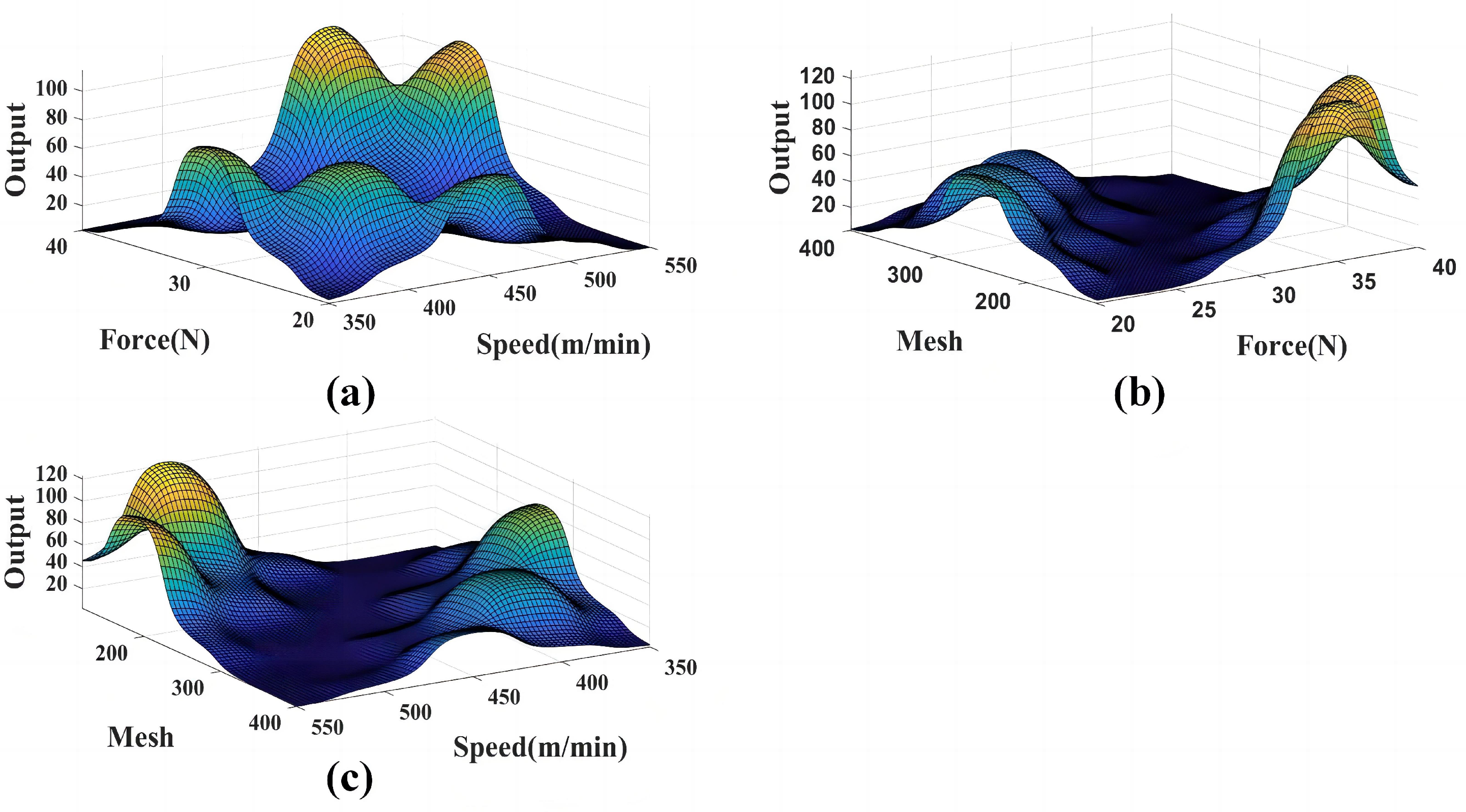
In this study, the three grinding factors, speed, mesh, and force, which were suggested to have the biggest effects on the material removal depth (MRD) in previous literature, are modeled. Firstly, orthogonal experiments were designed, using the Taguchi method, to reduce the number of experiments performed in order to find the optimal solution. Secondly, three-dimensional modeling of the robot hand-held blade grinding was applied to the actual grinding process. Finally, the regression model ANFIS was used to model the experimental results, and the influence of different parameters on material removal was studied. The reason for choosing ANFIS model will be discussed later. In contrast with the traditional linear modeling method, the relationship between the grinding tool and the workpiece was non-linear. The ANFIS method exploited in this paper is more suitable for practical situations. Therefore, it can predict the material removal depth without experiments.
The remainder of the paper is organized as follows: Section 2 introduces the theoretical basis of belt grinding and the basic structure of ANFIS. Section 3 conducts trajectory planning and orthogonal experimental design for the robot abrasive belt grinding steam turbine blade experiment. Moreover, the experimental results in Section 3 are analyzed and discussed in Section 4. Finally, the discussion results are summarized and conclusions drawn.

2. Preliminary

2.1. Belt Grinding

Belt grinding is a kind of elastic grinding processing method, which consists of the belt abrasive particles being fixed on the ring carrier with a certain elastic material, such as a cloth base or paper base, through a binder [22,23]. The belt is tightened by using at least two polymer rubber wheels, as shown in Figure 1. One of the wheels is the driving wheel, which is responsible for rotating the belt. Another wheel is the contact wheel, which is used to grind the workpiece with the abrasive belt. Therefore, the belt grinding is a composite process with a variety of functions, including rough grinding, fine grinding, and polishing. Since the soft contact wheel can make corresponding adjustments according to the shape of the workpiece, it can polish the workpiece with a free surface. Additionally, by modifying the abrasive belt grinding process parameters, we can alter the circumstances in which the abrasive belt comes into contact with the workpiece. This means that the amount of material removed during grinding can be controlled by changing the nonlinear behavior of the contact wheel and workpiece surface [24].

2.2. ANFIS Architecture

In the early 1990s, Jang applied fuzzy systems to adaptive network structures to obtain ANFIS. ANFIS can be divided into two parts: artificial neural network (ANN) and fuzzy inference system (FIS) [25]. Specifically, the two methods complement each other. On the one hand, FIS gives clear physical meaning to the nodes and weights of the neural network, avoiding the “black box” phenomenon in the traditional neural network processing. On the other hand, ANN has strong learning ability and can optimize the assumption rules of the fuzzy system in the process of data training, which solves the problem of unclear rules division in FIS operation [26,27]. This is helpful to the development of hybrid intelligent system network [28,29].
In general, ANFIS is usually divided into five layers. Its structure is shown in Figure 2, where x and y are inputs and f is an output.
Layer 1: In this layer, each square node i corresponds to a node function. As shown in formula (3):
O i 1 = v A i ( x ) , i = 1 , 2 o r O i 1 = v B j ( y ) , j = 1 , 2
where x (or y) are the two initial inputs and A i , B j represent the linguistic labels of the degree of ambiguity. The membership function of A (or B) can be arbitrary. The bell-shaped function v A i ( x ) (or v B j ( y ) ) is usually chosen, such as:
v A i ( x ) = 1 1 + x k i h i 2 m i
where { h i , k i , m i } is the set of parameters whose values control the shape of the membership function.
Layer 2: In this layer, each circle node ∏ is used to calculate the product of the signal passed into the node and then passed into the third layer.
O i 2 = u i = v A i ( x ) × v B i ( y ) , i = 1 , 2
Layer 3: In layer 3, there are circle nodes marked with N, which are normalized with the trigger intensity from the previous layer.
O i 3 = u i ¯ = u i i 2 u i = u i u 1 + u 2 , i = 1 , 2
Layer 4: This layer receives the normalized trigger intensity u i ¯ from the third layer.
O i 4 = u i ¯ f i = u i ¯ ( d i x + e i y + g i )
where { d i , e i , g i } is the parameter set.
Layer 5: This layer has only one circle node labeled ∑. Its function is to accumulate all the signals from the previous layer and output the result.
O i 5 = i u i ¯ f i = i u i f i i u i
In this way, a five-layer fuzzy adaptive network structure is constructed. We can also combine some of the layers to get a network structure with fewer layers. Likewise, we can perform weight normalization in the last layer of the network. Clearly, the assignment of node functions and the structure of the network are arbitrary as long as each node and each layer make sense and perform modular functions.

3. Main Results

3.1. Experimental Procedures

3.1.1. Materials

In this section, the turbine blade was used, which is one of the most delicate and important parts of the turbine. Particularly, the quality of the blade is directly related to the overall safety and reliability of the unit. The specific parameters of the blade are shown in the Computer Aided Design (CAD) drawing and physical drawing in Figure 3. The main component of the blade is 14Cr11MoV5 and the size is 65 × 12.5 × 11 mm. The aim of this experiment mainly addressed the material removal of the blade back arc surface by the grinding process parameters.

3.1.2. Experimental Setup

Figure 4 shows the experimental setup for robotic grinding of steam turbine blades. The six-degree-of-freedom ABB robot model used in the experiment was IRB 4600 45 / 2.05 . In Figure 4a shows that the robot places the blade on the belt grinder for grinding through the pneumatic gripper. In Figure 4b shows that the turbine blade is fixed on the pneumatic gripper. In Figure 4c shows coordinate measuring machine with probe used to measure the depth of cut across the grinded path at three different locations A, B and C. A six-axis sensor (ATI Omega 160) was installed at the end of the robot actuator to measure the grinding force in different directions when the robot ground the blade [6]. A pneumatic gripper was installed on the force sensor and clamped the blade. The grinding tool adopted a belt grinder, and the contact wheel of the belt grinder was 20 mm in diameter and 10 mm in width. The core material of the contact wheel was aluminum and the outer layer was elastic rubber with an average hardness of 13–18 HRC. The abrasive grains on the abrasive belt were alumina ceramics. Specifically, the parameters of the six-axis sensor are shown in Table 1. Additionally, it was crucial to confirm that the ground sample’s surface conditions were uniform and constant before the blade experiment was conducted.

3.1.3. Grinding Trajectory

The blade grinding workstation was built by the off-line simulation software RobotStudio. Moreover, the 3D model of the blade and grinding equipment was imported into the workstation. The grinding trajectory of the blade back arc was designed as shown in Figure 5. During the experiment, the force data between the workpiece and the contact wheel was sensed by the sensor and transmitted to the computer in real time by the DAQ (Data Acquisition) device. First, the blade back arc trajectory program to be polished on the RobotStudio was set. Second, the blade back arc trajectory program to be polished was transmitted to the actual robot teach pendant. Finally, the actual grinding path was fitted by manipulating the teaching point of the actual teach pendant.

3.1.4. Taguchi Experimental Design

In cases where the influence of each parameter of sand belt grinding on the sample was not clear, the Taguchi experimental design method was selected to show only the influence of each parameter on the grinding effect. Taguchi’s L25 orthogonal array (3 factors, 5 levels) was chosen to evaluate the impact of grinding parameters on the blade’s material removal depth. In this study, mesh number, rotational speed, and grinding force of the belt were used to analyze the influence of material removal. Table 2 shows the parameters set and levels used in the Taguchi experiment for specific sand belts. The three grinding parameters are presented in Table 3, using the L 25 orthogonal array. Furthermore, the removal depth of blade material was quantified according to the linear cutting depth of the blade profile. A coordinate measuring machine (CMM) was used to measure the removal amount of blade back arc material before and after grinding. The removal depth of the blade back arc was obtained as shown in Figure 4.

3.2. Experimental Conditions

The Taguchi experimental design method was used to study the belt grinding device based on grinding process parameters. Moreover, the following experimental conditions were kept constant during the grinding experiment to make the experiment controllable.
1. The position of the belt sander was kept unchanged in each experiment, so that the contact state of the blade and contact wheel was consistent during the experiment.
2. The experiment was carried out during the service life of the sand belt. Every time the sand belt was replaced with a new sand belt, the discarded blade was used to test the sand belt to prevent the excessive grinding amount of the new sand belt from affecting the accuracy of the experimental data.
3. The surface mass of the dorsal camber of the blade was uniform, about 9 µm.
4. The experiment was carried out in dry conditions.
5. Three measuring trajectories were taken from the grinding path in each experiment. Three measuring points were taken from each measuring line. The material removal depth before and after grinding was measured by CMM. Nine experimental data points were obtained.
According to the parameter combination of the Taguchi experiment, 25 tests were obtained, as shown in Table 3. A total of 225 grinding depth readings were obtained.

3.3. Data Acquisition for Grinding Depth

The three axes of the CMM are equipped with an air source brake switch and a micro-moving device, which can realize precision transmission of a single axis and adopt a high-performance data acquisition system. In this study, CMM was used to measure the material removal depth of the blades before and after grinding along the grinding path. Moreover, a confocal laser scanning microscope was used to scan the three straight trajectories (A, B and C) across the grinding path, in order to extract 2D contour of the grinding traces on the leaf surface. The depth of grinding is shown in Figure 6.
Blade back arc removal depth is defined as the distance difference between the deepest grinding point and the surface point. Each experiment was performed three times to guarantee the validity of the results. In addition, the blade thickness was measured at the same position before and after each experiment. The data values of 9 measurement points were obtained. Table 3 shows the average material removal depth (MRD) and corresponding SNR. The SNR is defined as follows:
S N R = 10 × l o g 10 ( 1 n i = 1 n 1 y i 2 )
where n is the number of values obtained in each Taguchi experiment and y i is all values obtained in each experiment. The greater the SNR, the greater the MRD. Therefore, the ideal level of process parameter values was the most significant level of SNR.

4. Results and Discussion

Figure 7 shows the average SNR plots for MRD for three factors and five levels. It can be seen from Figure 7 that the maximum removal depth of blade material was obtained when the speed of the sand belt was 550 m/min (level 5), the grinding force was 40 N (level 5) and the mesh number of the abrasive belt was 120 (level 1). As shown, the material removal ratio increased with the speed and grinding force of the belt, but decreased with the mesh number. In particular, when the belt speed rose, the area of contact between the abrasive belt and the workpiece expanded, increasing the amount of grinding [30]. As the grinding force increased, the friction between the contact wheel and the grinding area of the workpiece also increased. As a result, the workpiece and abrasive particles on the abrasive belt ground more vigorously, increasing MRD. In addition, the higher the mesh number, the smaller the abrasive particles in the sand belt and the smaller the grinding scratches caused to the workpiece during grinding, so the amount of grinding decreased as the mesh number of the sand belt increased.

4.1. Analysis of Variance

In order to understand, in detail, the effects of each parameter on the material removal depth (MRD) of the leaf back-arc, Analysis of Variance (ANOVA) was used. According to the ANOVA, the influence of each parameter on the MRD of blade material was compared, to determine the optimal MRD parameter combination more accurately. Table 4 shows the variance data of the Taguchi experimental results of the grinding process. There were three factors in this experiment, each of which had five levels. The results are shown in Table 4. When the significance level was 5 % , the confidence level was 95 % . According to Table 4, F 0.05 ( 4 , 12 ) = 3.259 was the distribution value of F. When the variation F was greater than 3.259 , the effect was significant. The degree of influence is Mesh > Force > Speed.
In order to reflect the interaction between each factor in the ANOVA process more intuitively, an interaction diagram was introduced. Figure 8 shows the interaction diagram of the influence of the three process parameters in the study of blade MRD [2].

4.2. ANFIS in Predicting MRD

Obviously, the prediction model developed in this study contained three input variables and one output variable, according to the characteristics of the input parameters and output parameters of the model, making it a standard multiple-input, single-output (MISO) system. The system structure of ANFIS is shown in Figure 9.

4.2.1. ANFIS Rules and Membership Function

ANFIS utilizes the neural network’s capacity for learning to implement the three fundamental processes of fuzzy control, fuzzy reasoning, and defuzzification. The self-adaptive tuning of the ANFIS system changes the membership function of each parameter of the model, and the optimal parameters of the membership function can be effectively calculated through self-learning, so that the designed fuzzy reasoning system can best simulate the desired input–output relations. Finding the fuzzy controller’s input and output variables is the first stage in the ANFIS system. Speed, force, and mesh were the three input parameters for the ANFIS model discussed in this article. The output was the blade’s material clearance depth (MRD). An ANFIS is a multiple-input single-output (MISO) system, as explained in this paper.
In this study, the Generalized Bell-shaped membership function was used to design 125 fuzzy rules for MRD prediction in the topology diagram of ANFIS, as shown in Figure 10. Three feature sets were used as inputs to build fifteen membership functions. For the purpose of fuzzifying the input features, each feature produced five member functions. The second level displays the 15 component functions in question. MF 1-1, …, and MF 1-5 were the membership functions for the input feature speed. The membership functions of the input feature Force were MF 2-1, …, and MF 2-5. The input feature Mesh had membership functions MF 3-1, …, and MF 3-5. The 225 data points in the sample used for this study were split between training and testing, with 70 % of the data being used for training and 30 % for testing. The “andMethod” and “orMethod” functions used in this paper to determine the second layer’s emission intensity were “Prod” and “Max”. By dividing the incoming signals, this function determined the emission intensity of each rule. For layers 3-5, “wtaver”, “prod”, and “max” were chosen as the appropriate “defuzz method”, “imp method”, and “agg method” in this work, respectively. The Generalized Bell-shaped membership function was chosen as the membership function. It was decided to use the least squares estimation-gradient descent method for the overall learning rule algorithm. The ANFIS parameter is shown in Table 5.
Figure 11 shows the membership function images of three grinding input parameters obtained by training the generalized bell-shaped membership function before and after training. The membership function is a function used to describe the degree to which a variable belongs to a fuzzy set, in which the possible value range is ( 0 ,   1 ) . The membership function used in this paper was generalized bell-shaped membership (Gbellmf). The three membership functions with grinding input parameters obtained by training the Gbellmf can be observed.
It can be seen from Figure 11 that the shape of the membership function of the input parameters changed significantly before and after training. By analyzing the generalized bell-shaped membership functions before and after training, it was found that, among the three process parameters, the most influential factor for material removal was mesh, followed by force and speed. The results were consistent with the results of variance analysis in Section 4.1.

4.2.2. Training Network and Prediction Performance

The interdependencies between the input and output parameters of the control surface, being led by different rules in a specific universe, are shown in Figure 12. Specifically, fuzzy logic toolbox was utilized in the MATLAB environment to implement these rules. In Figure 12a the control surface shows the interdependence among MRD, Force and Speed. In Figure 12b the control surface shows the interdependence among MRD, Force, and Mesh. In Figure 12c the control surface shows the interdependence among MRD, Mesh, and Speed.
The ANFIS model was trained using experimental data, then tested. Figure 13 compares the anticipated and actual values. The prediction results show that the designed ANFIS robot abrasive belt grinding material removal prediction model had decent precision.

4.3. ANN, SVR and RF

In order to verify the scientificity of the ANFIS material removal model we developed, three other regression models (ANN, SVR and RF) were tested with the same data. The model parameters for ANN, SVR and RF were carefully chosen to obtain the best accuracy, giving objective and unbiased comparative results.
In this study, the model was trained using 70 % of the data set, and tested using the remaining 30 % of the data set. The architecture and training process of an ANN model affects its accuracy. One neuron is employed in the output layer to represent MRD, whereas three neurons in the ANN input layer represent the three input parameters. In regard to ANN, nonlinear structures between input and output are built using back-propagation neural networks. First, the network’s weights were modified at the output neurons during the learning phase. Second, the weights were inversely adjusted at the hidden layer throughout the training process, up till the predicted error was obtained. Finally, the modeling results were produced using the ANN toolbox in the MATLAB software and the hyperbolic tangent sigmoid transfer function. The back-propagation method used by ANN was Bayesian regularization and the remaining data was used for model verification.
For SVR, first it is necessary to define the datasets and predictors. Then, the kernel function is fitted to be Gaussian and an ideal model chosen to train the predictor and response of the input data [31]. Moreover, the Bayesian optimization model was used to train the model in the MATLAB environment. Finally, the test set was used to validate the model. The random forest regression algorithm’s fundamental tenet is to construct a data sample with a sample size of N, having a retrieval of N times, and then to create a sample set ( x 1 ,   x 2 x n ) . There are M attributes for the sample x i . When the decision tree needs to be split at each node, m attributes are chosen at random from the M attributes, where mM. The split attribute of the node is then chosen using information obtained from among m attributes. Each node must be divided until it can no longer be divided as part of the decision tree construction process. After creating a substantial number of decision trees, a random forest is created.
Finally, the mean absolute percentage error ( M A P E ) was used to assess the accuracy of the ANFIS, ANN, SVR, and RF models in comparison. Table 6 shows the partial prediction data and error percentage of the four models. M A P E is defined as:
M A P E = 100 % n k = 1 n M k P k M k
where M k and P k are the measured and predicted grinding quantities and n is the total number of samples used [32].
The M A P E of ANFIS, ANN, SVR, and RF were 3.976 % , 5.713 % , 12.717 % , and 16.635 % , respectively. Notice that ANN was close to the prediction result of ANFIS and that the RF performance was relatively poor [21]. The absolute percentage error (APE) of the four models is shown in Figure 14.
As shown in Figure 14, the absolute percentage error (APE) of the ANFIS model was the smallest, compared to the other three models. ANN and ANFIS had similar APEs. The M A P E of the predicted value of the ANFIS model was 3.976 % and the minimum APE was 0.27 % . The findings indicate that the suggested ANFIS model is reliable and accurate for predicting material removal depth during grinding.

5. Conclusions

In this study, a method based on Taguchi experimental design was analyzed and demonstrated. The influences of various process parameters on material removal of robotic belt grinding were studied. In the Taguchi experiment, five-level values of force, speed, and mesh for three factors were applied. According to the analysis and discussion of the experimental results, the following general conclusions can be drawn:
1. Adaptive Neuro-Fuzzy Inference System (ANFIS) was applied to predict the removal depth of robot belt grinding material. Based on ANFIS, a MISO system with different grinding parameters affecting MRD was established and verified by practical data. The prediction outcomes demonstrated the high accuracy of the ANFIS robot abrasive belt grinding material removal prediction model, with a M A P E of only 3.976 % .
2. Based on the main effect analysis diagram in Figure 7, it can be concluded that speed: 550 m/min, force: 40 N, and mesh: 120 were the parameters corresponding to the maximum MRD.
3. The same data set was applied to three models, ANN, SVR, and RF, and their M A P E values compared with ANFIS. The M A P E values of ANFIS, ANN, SVR, and RF were 3.976 % , 5.713 % , 12.717 % , and 16.635 % , respectively. As can be observed, ANFIS significantly outperformed the other models, while RF performed poorly.
4. ANFIS is flexible and can be used as an alternative to traditional modeling techniques after a large amount of data training. After a suitable fuzzy inference model is established, the depth of material removal can be analyzed without actual experiments. Therefore, the model may be used for actual grinding, and the quantity of grinding can be monitored online.

Author Contributions

H.J., D.C. and X.L. have generated the new research idea, done investigations and conducted experiments; H.J., Y.X., X.L. and J.C. have conducted the experiments and writing original draft; C.B. supported the material and equipment. H.J. and D.C. revised the manuscript. All authors have read and agreed to the published version of the manuscript.

Funding

This research was funded by Zhejiang Province’s “Leading Goose” R&D Program: Key Technology and System Engineering R&D Project of Surface Grinding and Polishing Robot, China, [NO. 2022C01096].

Institutional Review Board Statement

Not applicable.

Informed Consent Statement

Not applicable.

Data Availability Statement

Restrictions apply to the availability of this data. The data were obtained from Wahaha Intelligent Robotics Company and are available from the corresponding author with the permission of Wahaha Intelligent Robotics Company.

Conflicts of Interest

The authors declare that they have no conflict of interest.

References

  1. Korchak, S. Performance of the Process of Grinding Steel Parts; Mashinostroenie (Mechanical Engineering): Moscow, Russia, 1974; p. 230. [Google Scholar]
  2. Zhu, D.; Feng, X.; Xu, X.; Yang, Z.; Li, W.; Yan, S.; Ding, H. Robotic grinding of complex components: A step towards efficient and intelligent machining–challenges, solutions, and applications. Robot. Comput. Integr. Manuf. 2020, 65, 101908. [Google Scholar] [CrossRef]
  3. Zhang, X.; Cabaravdic, M.; Kneupner, K.; Kuhlenkoetter, B. Real-time simulation of robot controlled belt grinding processes of sculptured surfaces. Int. J. Adv. Robot. Syst. 2004, 1, 12. [Google Scholar] [CrossRef] [Green Version]
  4. Wu, S.; Kazerounian, K.; Gan, Z.; Sun, Y. A material removal model for robotic belt grinding process. Mach. Sci. Technol. 2014, 18, 15–30. [Google Scholar] [CrossRef]
  5. Yang, Z.; Chu, Y.; Xu, X.; Huang, H.; Zhu, D.; Yan, S.; Ding, H. Prediction and analysis of material removal characteristics for robotic belt grinding based on single spherical abrasive grain model. Int. J. Mech. Sci. 2021, 190, 106005. [Google Scholar] [CrossRef]
  6. Lv, Y.; Peng, Z.; Qu, C.; Zhu, D. An adaptive trajectory planning algorithm for robotic belt grinding of blade leading and trailing edges based on material removal profile model. Robot. Comput. Integr. Manuf. 2020, 66, 101987. [Google Scholar] [CrossRef]
  7. Bigerelle, M.; Hagege, B.; El Mansori, M. Mechanical modelling of micro-scale abrasion in superfinish belt grinding. Tribol. Int. 2008, 41, 992–1001. [Google Scholar] [CrossRef]
  8. Wang, W.; Liu, F.; Liu, Z.; Yun, C. Prediction of depth of cut for robotic belt grinding. Int. J. Adv. Manuf. Technol. 2017, 91, 699–708. [Google Scholar] [CrossRef]
  9. Hammann, G. Modellierung des Abtragsverhaltens Elastischer, Robotergeführter Schleifwerkzeuge; Springer: Berlin/Heidelberg, Germany, 2013; Volume 123. [Google Scholar]
  10. Preston, F. The theory and design of plate glass polishing machines. J. Glass Technol. 1927, 11, 214–256. [Google Scholar]
  11. Pandiyan, V.; Caesarendra, W.; Tjahjowidodo, T.; Praveen, G. Predictive modelling and analysis of process parameters on material removal characteristics in abrasive belt grinding process. Appl. Sci. 2017, 7, 363. [Google Scholar] [CrossRef]
  12. Zhe, H.; Jianyong, L.; Yueming, L.; Meng, N.; Wengang, F. Investigating the effects of contact pressure on rail material abrasive belt grinding performance. Int. J. Adv. Manuf. Technol. 2017, 93, 779–786. [Google Scholar] [CrossRef]
  13. Xiao, G.; Song, K.; Liu, S.; Wu, Y.; Wang, W. Comprehensive investigation into the effects of relative grinding direction on abrasive belt grinding process. J. Manuf. Process. 2021, 62, 753–761. [Google Scholar] [CrossRef]
  14. Pandiyan, V.; Caesarendra, W.; Glowacz, A.; Tjahjowidodo, T. Modelling of material removal in abrasive belt grinding process: A regression approach. Symmetry 2020, 12, 99. [Google Scholar] [CrossRef] [Green Version]
  15. Gill, S.S.; Singh, J. An Adaptive Neuro-Fuzzy Inference System modeling for material removal rate in stationary ultrasonic drilling of sillimanite ceramic. Expert Syst. Appl. 2010, 37, 5590–5598. [Google Scholar] [CrossRef]
  16. Khalick Mohammad, A.E.; Hong, J.; Wang, D. Polishing of uneven surfaces using industrial robots based on neural network and genetic algorithm. Int. J. Adv. Manuf. Technol. 2017, 93, 1463–1471. [Google Scholar] [CrossRef]
  17. Gao, K.; Chen, H.; Zhang, X.; Ren, X.; Chen, J.; Chen, X. A novel material removal prediction method based on acoustic sensing and ensemble XGBoost learning algorithm for robotic belt grinding of Inconel 718. Int. J. Adv. Manuf. Technol. 2019, 105, 217–232. [Google Scholar] [CrossRef]
  18. Pandiyan, V.; Shevchik, S.; Wasmer, K.; Castagne, S.; Tjahjowidodo, T. Modelling and monitoring of abrasive finishing processes using artificial intelligence techniques: A review. J. Manuf. Process. 2020, 57, 114–135. [Google Scholar] [CrossRef]
  19. Pandiyan, V.; Caesarendra, W.; Tjahjowidodo, T.; Tan, H.H. In-process tool condition monitoring in compliant abrasive belt grinding process using support vector machine and genetic algorithm. J. Manuf. Process. 2018, 31, 199–213. [Google Scholar] [CrossRef]
  20. Kecman, V. Learning and Soft Computing: Support Vector Machines, Neural Networks, and Fuzzy Logic Models; MIT Press: Cambridge, MA, USA, 2001. [Google Scholar]
  21. Caesarendra, W.; Wijaya, T.; Tjahjowidodo, T.; Pappachan, B.K.; Wee, A.; Roslan, M.I. Adaptive neuro-fuzzy inference system for deburring stage classification and prediction for indirect quality monitoring. Appl. Soft Comput. 2018, 72, 565–578. [Google Scholar] [CrossRef]
  22. He, Z.; Li, J.; Liu, Y.; Yan, J. Single-grain cutting based modeling of abrasive belt wear in cylindrical grinding. Friction 2020, 8, 208–220. [Google Scholar] [CrossRef] [Green Version]
  23. Zou, L.; Liu, X.; Huang, Y.; Fei, Y. A numerical approach to predict the machined surface topography of abrasive belt flexible grinding. Int. J. Adv. Manuf. Technol. 2019, 104, 2961–2970. [Google Scholar] [CrossRef]
  24. Zou, L.; Wang, T.; Wang, C.; Li, Z.; Wu, Y.; Huang, Y. Modelling and analysis of the effect of nonlinear time-varying contact deformation on flexible precision grinding process. Int. J. Adv. Manuf. Technol. 2021, 115, 77–89. [Google Scholar] [CrossRef]
  25. Jain, A.K.; Mao, J.; Mohiuddin, K.M. Artificial neural networks: A tutorial. Computer 1996, 29, 31–44. [Google Scholar] [CrossRef] [Green Version]
  26. Luis Pérez, C. A Proposal of an Adaptive Neuro-Fuzzy Inference System for Modeling Experimental Data in Manufacturing Engineering. Mathematics 2020, 8, 1390. [Google Scholar] [CrossRef]
  27. Marani, M.; Songmene, V.; Zeinali, M.; Kouam, J.; Zedan, Y. Neuro-fuzzy predictive model for surface roughness and cutting force of machined Al–20 Mg2Si–2Cu metal matrix composite using additives. Neural Comput. Appl. 2020, 32, 8115–8126. [Google Scholar] [CrossRef]
  28. Jang, J.S. ANFIS: Adaptive-network-based fuzzy inference system. IEEE Trans. Syst. Man Cybern. 1993, 23, 665–685. [Google Scholar] [CrossRef]
  29. Jang, J.S.R.; Sun, C.T.; Mizutani, E. Neuro-fuzzy and soft computing-a computational approach to learning and machine intelligence [Book Review]. IEEE Trans. Autom. Control 1997, 42, 1482–1484. [Google Scholar] [CrossRef]
  30. Ren, J.; Hao, M.; Liang, G.; Wang, S.; Lv, M. Study of subsurface damage of monocrystalline nickel in nanometric grinding with spherical abrasive grain. Phys. B Condens. Matter 2019, 560, 60–66. [Google Scholar] [CrossRef]
  31. Smola, A.J.; Schölkopf, B. A tutorial on support vector regression. Stat. Comput. 2004, 14, 199–222. [Google Scholar] [CrossRef] [Green Version]
  32. Pei, L.; Sun, Z.; Yu, T.; Li, W.; Hao, X.; Hu, Y.; Yang, C. Pavement aggregate shape classification based on extreme gradient boosting. Constr. Build. Mater. 2020, 256, 119356. [Google Scholar] [CrossRef]
Figure 1. Principle of belt grinding process.
Applsci 13 04248 g001
Figure 2. Structure of ANFIS.
Applsci 13 04248 g002
Figure 3. Computer Aided Design (CAD) and physical drawing of the workpiece used for the grinding experiment.
Applsci 13 04248 g003
Figure 4. Experimental setup for (a) robotic grinding device, (b) blade, (c) grinding depth measurement device.
Applsci 13 04248 g004
Figure 5. Off-line trajectory planning of blade polishing.
Applsci 13 04248 g005
Figure 6. 2D contour of the removal depth of blade grinding material.
Applsci 13 04248 g006
Figure 7. Average signal-to-noise ratio (SNR) of MRD.
Applsci 13 04248 g007
Figure 8. Two-way interaction between speed, force and mesh and their influences on MRD at different initial parameter levels.
Applsci 13 04248 g008
Figure 9. Input and output display of ANFIS model for abrasive belt grinding.
Applsci 13 04248 g009
Figure 10. Topological structure of ANFIS.
Applsci 13 04248 g010
Figure 11. Image of the generalized bell-shaped membership function before and after training for each input parameter.
Applsci 13 04248 g011
Figure 12. The control surface of the fuzzy model shows the interdependence between (a) MRD, Force (N), and Speed (m/min); (b) MRD, Force (N), and Mesh; (c) MRD, Speed (m/min), and Mesh.
Applsci 13 04248 g012
Figure 13. Comparison between experimental grinding depth and ANFIS prediction.
Applsci 13 04248 g013
Figure 14. Absolute percentage error (APE) of the four models.
Applsci 13 04248 g014
Table 1. Parameters of the ATI Omega160 sensor.
F x / F y ( N ) F z ( N ) M x (N·M) M y / M z (N·M)
Measuring range±1500±3750±240±240
Measurement accuracy1/161/81/1601/160
Uncertainty of measurement1.50%1.25%1.00%1.25%
Table 2. Grinding parameters and the level of abrasive belt.
ParametersUnitLevels
1 2 3 4 5
Mesh-120180240320400
Speedm/min350400450500550
ForceN2025303540
Table 3. Partial Taguchi experiments and corresponding cutting depth and signal-to-noise ratio (SNR).
Experiment No.Speed (m/min)Force (N)MeshMRD (µm)SNR (db)
13502012094.4939.45
23502518087.3038.78
33503024079.9438.00
43503532067.5536.62
53504040055.5734.80
64002018081.1638.19
74002524073.9637.34
84003032060.9835.58
94003540048.8333.72
1040040120132.8242.44
114502024068.2036.62
124502532054.6334.74
134503040042.4132.97
1445035120126.7842.07
1545040180119.6841.52
165002032051.1734.16
175002540041.4432.34
1850030120122.8541.79
1950035180115.3241.19
2050040240108.5640.61
215502040033.6430.46
2255025120116.9941.34
2355030180106.8940.59
2455035240102.6440.26
255504032090.2739.14
Table 4. Analysis of variance results from MRD.
Machining ParameterDegrees of FreedomSum of SquaresMean SquareF Ratio F 0.05 (4, 12)
Speed42.9980.7493.4103.259
Force447.30311.82553.8803.259
Mesh4231.25057.812263.4103.259
Error122.6340.219-3.259
Total24284.185--3.259
Table 5. ANFIS parameters.
ParameterValue
Neuron level3
Size of input data set225
Training set 70 %
Testing set 30 %
andMethodProd
orMethodMax
defuzzificationWtaver
AggregationMax
Maxepoch160
Membership functionGbellmf
Clustering TypeGrid Partitioning
Learning rulesLeast square estimation-gradient decent algorithm
Table 6. Partial measured and predicted values of the four models.
Cutting Depth (µm)ANFISANNSVRRF
Predicted MRD (µm)Error (%)Predicted MRD (µm)Error (%)Predicted MRD (µm)Error (%)Predicted MRD (µm)Error (%)
92.4993.771.3895.313.0592.350.1581.2512.15
78.6778.970.3878.540.1777.641.3167.5414.15
74.3572.871.9974.620.3676.272.5868.328.11
47.9448.070.2746.522.9646.213.6155.1415.02
133.21132.140.80131.671.16130.262.21117.3611.90
40.6541.973.2543.236.3545.2811.3947.5116.88
120.67118.701.63117.652.50122.341.38105.2412.79
123.54122.071.19120.322.61130.485.62132.987.64
106.74105.930.76108.942.06101.365.0499.217.05
62.4560.243.5459.125.3364.823.8053.1514.89
Disclaimer/Publisher’s Note: The statements, opinions and data contained in all publications are solely those of the individual author(s) and contributor(s) and not of MDPI and/or the editor(s). MDPI and/or the editor(s) disclaim responsibility for any injury to people or property resulting from any ideas, methods, instructions or products referred to in the content.

