Gaussian Mutation Specular Reflection Learning with Local Escaping Operator Based Artificial Electric Field Algorithm and Its Engineering Application

Abstract

During the contribution of a metaheuristic algorithm for solving complex problems, one of the major challenges is to obtain the one that provides a well-balanced exploration and exploitation. Among the possible solutions to overcome this issue is to combine the strengths of the different methods. In this study, one of the recently developed metaheuristic algorithms, artificial electric field algorithm (AEFA), has been used, to improve its converge speed and the ability to avoid the local optimum points of the given problems. To address these issues, Gaussian mutation specular reflection learning (GS) and local escaping operator (LEO) have been added to the essential steps on AEFA and called GSLEO-AEFA. In order to observe the effect of the applied features, 23 benchmark functions as well as engineering and real-world application problems were tested and compared with the other algorithms. Friedman and Wilcoxon rank-sum statistical tests, and complexity analyses were also conducted to measure the performance of GSLEO-AEFA. The overall effectiveness of the algorithm among the compared algorithms obtained in between 84.62–92.31%. According to the achieved results, it can be seen that GSLEO-AEFA has precise optimization accuracy even in changing dimensions, especially in engineering optimization problems.

1. Introduction

The development of optimization techniques is crucial since there are many optimization issues that need to be resolved in the real world. The majority of these techniques depend on being able to find derivatives of the involved functions. However, for various reasons, the derivatives might be occasionally challenging to get. Those problems include electromagnetic problems which were difficult to tackle because of limitations in computational sources [1]. However due to the advancement of computers many different optimization methods are applied to solve these kind of scattering problems [2,3]. Metaheuristic algorithms which are a crucial component of derivative-free approaches are becoming more and more popular due to their effective searching capabilities. Metaheuristic algorithms can be categorized into groups based on what they imitate or mimic. Swarm intelligence mimicking algorithms are gaining popularity due to a variety of features including powerful searching capabilities, straightforward implementation, minimal parameters, and the capacity to avoid becoming stuck in a sub-optimal position [4]. The search agents collaborate and share information with one another in these algorithms, ensuring that the search space’s information is effectively used. This allows the entire swarm to advance toward more promising areas of the search space. Numerous swarm intelligence techniques have been presented in several of the literatures and used to solve practical issues during the last few decades [5,6,7,8,9,10]. Physics law mimicking algorithms imitate the physical principles that control how agents interact with one another and their search environment. These principles include the principle of gravity, light, and refraction [11]. They are being implemented in several areas to solve engineering challenges [12,13,14,15].

Evolution theory mimicking algorithms through various combination and permutations of populations obtain the best solution. The main benefit of this method is that the individuals with the best solutions combine to create the next generation [16,17,18,19]. The exploitation and exploration patterns of behavior are basically the patterns the metaheuristic algorithms will follow as it advances towards the optimal solution. The discovery of new search space areas is called exploration. Exploitation is the procedure of locating and investigating the most promising areas in the hunt for potentially superior solutions [20]. Any metaheuristic algorithms share a potential problem in trying to maintain an adequate balance between these two patterns since they contradict each other [21].

In 2019, Anita and Yadav suggested the artificial electric field algorithm (AEFA) [22]. The leadership influence of the lead particle, in other words, the particle with the strongest charge and the behavior of the other particles as they are drawn along the search area by the lead particle, serve as the foundation for the search mechanism of the AEFA. This approach ensures that the algorithm is able to exploit promising areas for the best solution consistently [15]. AEFA has earned a reputation and has been effectively applied to several sectors in recent years due its various benefits, including ease of implementation, low computing cost, and great search efficiency. A few of the areas in which AEFA has proved a useful optimization algorithm are tumor detection [23], multi-objective problem [24], parameter extraction for photovoltaic model [25], assembly line balancing optimization problem [26], and feature selection [27]. Despite AEFA being applicable in many areas, prior research has revealed that it has significant shortcomings such as premature convergence, exploration and exploitation imbalance, and a propensity to become stuck at sub-optima [15,28,29], which are also present in other metaheuristic algorithms. However, the attraction force mechanism of the AEFA has a significant impact on population diversification. In the typical AEFA, a dominating particle directs the search process. This causes the population to gather around a single particle. As a result, this particle’s information is crucial for the population, and when it results in a less-than-ideal solution, it lowers the search efficiency of the algorithm.

The absence of techniques for population mutation, the propensity to enter sub optimal and delayed convergence are some of the issues that restrict the practical uses of AEFA, despite the fact that it is an effective optimization technique. To address the shortcomings of AEFA, researchers have produced a number of variants in recent years. To improve the search efficiency and stability of AEFA, the artificial electric field algorithm with pattern search algorithm (AEFA-PS) was suggested for open switch network problem. It was shown to be capable of getting objective function fitness values of greater quality [30]. The improved artificial electric field algorithm (IAEFA) developed a unique method for calculating the electrostatic force that solved the limitations of AEFA such as early convergence and low search performance. The performance of IAEFA was assessed using 18 different test functions and it was discovered to be a more effective and efficient at solving the optimization problems [31]. Although AEFA has limited global search capabilities, it offers excellent local search capabilities. In order to overcome this, the adaptive search sine-cosine algorithm with artificial electric field algorithm (SC-AEFA) technique was created to dynamically balance the global and local search abilities of the algorithm. Experiments demonstrated the greater performance was achieved [15]. In order to overcome the problem of entering the sub-optimality in the original AEFA, the Moth Levy adopted artificial electric field algorithm (ML-AEFA) was proposed. In comparison to other algorithms, experiments revealed superior performance [32]. By instantly introducing the fittest particles into the population for the following generation and keeping the best particles from one iteration to the next, the elitism strategy boosts the potential of AEFA for optimization. Studies demonstrate the higher performance of AEFA [33].

The primary driving force for this study is to solve the aforementioned issues. Our goal is to successfully strike a balance between the capacity for exploration and exploitation and the enhancement of population variety. The suggested AEFA is based on Gaussian mutation specular reflection (GS) and local escaping operator (LEO) called GSLEO-AEFA. Firstly, the convergence efficiency of an algorithm is impacted by the low diversity and the use of starting agents that are randomly generated. The specular reflection learning approach is applied in this study to produce high-quality starting populations. Gaussian mutation is introduced for the mutation of the new population to further increase the variety of the starting population. Additionally, the local escape operator mechanism is added to the algorithm to update particle positions and prevent the population from settling into sub-optimal, thereby enhancing the capabilities for global search. It is also designed to advance the population toward the global optimum and achieve equilibrium between exploration and exploitation.

During the forming of the GSLEO-AEFA, no modifications have been applied on the combined methods except the opposition-based learning (OBL). In this paper, we proposed an enhanced form of OBL called Gaussian mutation-based specular reflection (GS) and applied it to the standard AEFA algorithm. OBL is a technique that generates diverse candidate solutions in multimodal problems by having each solution learn from its opposite candidate [34]. It is a principle that inspired from the development of specular reflection. Specular reflection models the reflection of light in physics [35]. Our approach involves introducing the mutated form of specular reflection using Gaussian mutation only during the population initialization stage to enhance the diversity. This differs from the OBL introduced by Alkayem et al. [36] which is applied at initialization and later during iteration, and the quasi-based opposition learning introduced by Alkayem et al. [37] which aims to improve convergence speed and escape local optima during both initialization and iteration.

The main contributions of this paper are:

• We introduce a GSLEO-AEFA algorithm to improve the performance and balance in between exploitation and exploration phases of the original AEFA.
• We introduce a Gaussian mutation with specular learning strategy to enhance population diversity and as a new strategy for population initialization.
• We introduce a local escaping operator as a method for avoiding stagnation in local optimal.
• We use real world engineering problems to evaluate GSLEO-AEFA.

The remainder of the paper is organized as follows. Section 2 contains the detailed explanations of the artificial electrical field optimization algorithm (AEFA) and the proposed Gaussian mutation specular refraction learning with local escaping operator based AEFA (GSLEO-AEFA). Section 3 shows the experimental results and discussions of GSLEO-AEFA with its counterpart algorithms using 23 benchmark functions and engineering problems. Some necessary analyses such as convergence trajectory analysis, complexity analysis, diversity analysis and statistical analyses are implemented and discussed here. Lastly, in Section 4 the conclusion of the study is given.

2. Methodology

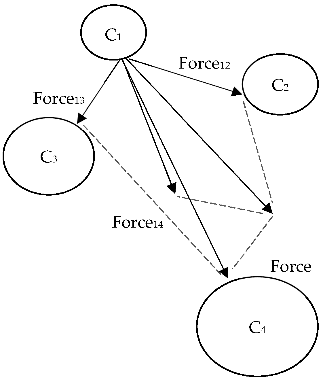
2.1. Artificial Electric Field Algorithm (AEFA)

The artificial electric field algorithm (AEFA) imitates how charged particles flow in an electrostatic field. The repulsive force between charged particles is ignored by AEFA, and only the attractive force between particles is considered. This enables surrounding low-charge particles to be drawn by high-charge particles in the electric field.

Each charged particle in the search area represents a potential solution. The charge associated with a particle determines the quality of the solution. The solution is closer to the ideal solution as the charge increases. Figure 1 illustrates the motion of the charged particles where the circles represent the several particles as they are located across the electric field and the circle sizes represent the quantity values of the charges that the particles carry. Particle $C_1$ experiences a force named $\mathrm{Force}$ in Figure 1 and it accelerates in the direction of the other three charged particles as a result of being attracted towards them. As can be seen, $C_4$ has the highest charge and it strongly attract $C_1$. As a result, the direction of the force acting on $C_1$ is more closely drawn towards the direction of $C_4$. Particles in the search area with low charges would therefore gravitate towards those with high charges throughout the AEFA iteration phase, enabling the algorithm to reach to the best outcome [22,38].

Equations (1) and (2) explains the theoretical formulation of the AEFA [39].

$$Ve{l}_i^{t+1}=\mathrm{r}\times Ve{l}_i^t+acc{l}_i^t$$

(1)

$$P_i^{t+1}=P_i^t+Ve{l}_i^t$$

(2)

The $i$th charged particle’s velocity is given as $Ve{l}_i^{t+1}$ and the location of that particle is represented with $P_i^{t+1}$ using Equations (1) and (2). The velocity and current position can be updated at iteration $t+1$; $r$ denotes random number in the range [0, 1]. The acceleration of particle at the $t$ iteration is denoted by $acc{l}_i^t$.

The formula of acceleration when a particle is exposed to an electric fields’ force is defined in Equation (3) as follows by Newton’s second law,

$$acc{l}_i^t=\frac{C_i^t\times E{F}_i^t}{m_i^t}$$

(3)

where $m_i^t$ denote mass of a particle and $C_i^t$ represent the charge of a particle. The electric field intensity of the $i$th particle at iteration $t$ is expressed as,

$$E{F}_i^t=\frac{Forc{e}_i^t}{C_i^t}$$

(4)

The charged particle’s resulting force in the search space is given as,

$$Forc{e}_i^t={{\displaystyle \sum }}_{j=1,j\ne i}^N\mathrm{r}\times Forc{e}_{ij}^t$$

(5)

According to the Coulomb’s force, the resulting force exacted on particle $i$ by $j$ is computed as follows.

$$Forc{e}_{ij}^t=K^t\times \frac{C_i^t\times C_j^t\times \left(P_{\mathrm{best}}^t-P_i^t\right)}{R_{ij}^t+\epsilon }$$

(6)

$$R_{ij}=\Vert P_i\left(t\right),P_j{\left(t\right)\Vert }_2$$

(7)

$$K^t=K_0\times \exp \left(-\alpha \times \frac{\mathrm{iteration}}{{\mathrm{Max}}_{\mathrm{iteration}}}\right)$$

(8)

In Equation (7), $R_{ij}$ denote the distance between two agents $i$ and $j$, $P_{\mathrm{best}}^t$ is the particle with ideal solution at the iteration $i$, and $\epsilon$ denote a very tiny positive value. The Coulomb constant $K_0$ is initially set at 500 and drops by a factor of 30 which is denoted as $\alpha$ in Equation (8) at every iteration. This progressive decline enables the algorithm to start with a global search and switch to a local search later on.

Each particles charge $C_i^t$ at a given iteration as given as follows,

$$C_i^t=\frac{c{q}_i^t}{{{\displaystyle \sum }}_{i=1}^N\mathrm{c}{q}_i^t}$$

(9)

$$c{q}_i^t=\exp \left(\frac{fi{t}_i^t-\mathrm{worst}\left(t\right)}{\mathrm{best}\left(t\right)-\mathrm{worst}\left(t\right)}\right)$$

(10)

In Equation (9), the total number of particles which is represented by $N$, the normalization of $c{q}_i^t$ is denoted by $C_i^t$, where $c{q}_i^t$ is the charge of the $i$th particle. In Equation (10), $\mathrm{best}\left(t\right)$ and $\mathrm{worst}\left(t\right)$ denote the ideal and worst fitness values at the $t$th iteration, respectively. $fi{t}_i^t$ is the fitness value of the $i$th particle. Using a greedy method, the algorithm updates the positions particles at each iteration.

$$P_i^{t+1}=\{\begin{array}{ll}{P}_i^t\hfill & \mathrm{when}\mathrm{fit}\left({\mathit{P}}_{\mathit{i}}^{\mathit{t}}\right)<\mathrm{fit}\left(P_i^{t+1}\right)\hfill \\ P_i^{t+1}\hfill & \mathrm{when}\mathrm{fit}\left(P_i^t\right)\ge \mathrm{fit}\left(P_i^{t+1}\right)\hfill \end{array}$$

(11)

The position of the individual in the following generation is determined by its fitness, according to Equation (11). The individual’s position is unaffected, if it has less fitness value than the fitness value of newly generated individual. If not, its position is re-adjusted. The pseudocode of AEFA can be seen in the following Algorithm 1.

Algorithm 1 Artificial Electric Field Algorithm (AEFA)

Initialize the population of size $N$ within search range $\left[P_{\min },P_{\max }\right]$ Set the Initial $Ve{l}_i^t$ to 0 Calculate fitness value for all particles Set iteration $i\leftarrow 1$ while stopping requirement is not met do         Compute $K^t$$,\mathrm{best}\left(t\right)$ $\mathrm{and}\mathrm{worst}\left(t\right)$                 for $i\leftarrow 1$ to $N$ do                      Calculate fitness values                      Calculate the total force in each direction Equation (5)                      Calculate acceleration Equation (3) $Ve{l}_i^{t+1}\leftarrow \mathrm{r}\times Ve{l}_i^t+acc{l}_i^t$ $P_i^{t+1}\leftarrow P_i^t+Ve{l}_i^t$              end for end while

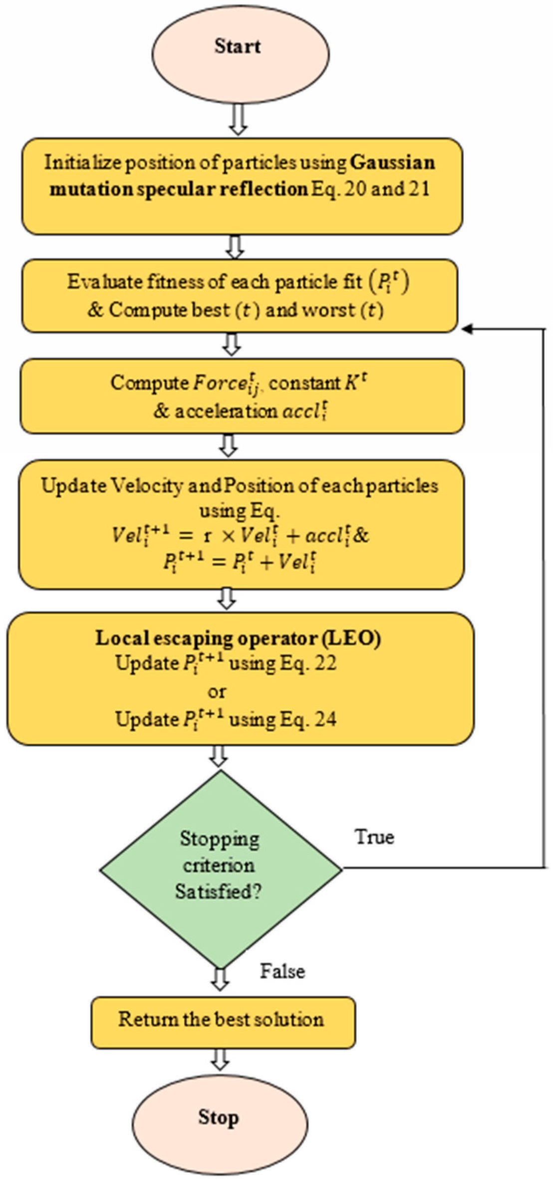
2.2. Proposed GSLEO-AEFA

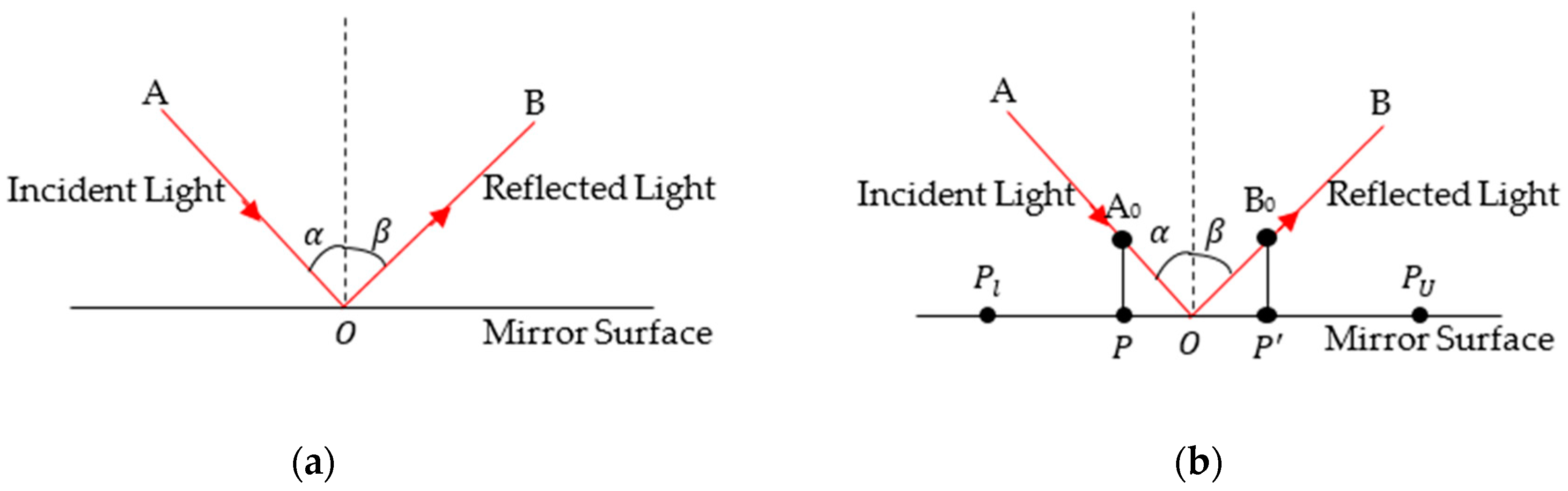
2.2.1. Population Initialization Using Gaussian Mutation Specular Reflection Learning (GS)

The variety of the starting agents has a major influence on the convergence rate and solution precision of metaheuristic algorithms [40]. However, AEFA frequently uses random initialization to generate the starting population. This initialization strategy lacks prior information of the search space, which might impact the updating method of the search agents. The population has the possibility of moving away from the ideal solution if the optimal solution is situated in the opposite location from where the randomly produced individuals are positioned. Solutions generated by the specular reflection learning (SRL) technique has been shown to outperform those produced only by random approaches [41]. This study introduces the application of specular reflection learning for the initialization of population and will produce an opposing population of the initial population. Afterwards, the Gaussian mutation (GM) process will be applied to the newly generated population to improve population variety from the generated agents. It is decided which individuals should be retained by comparing their fitness values with that of the original individuals.

Due to its superior performance, opposition-based learning (OBL) is frequently employed to enhance metaheuristic algorithms [42]. OBL uses simultaneous examination of potential solution and its opposing solution to promote rapid convergence. Within the range [$lb,ub$], the opposing value of $p$ is defined as follows:

$$p^{\ast }=lb+ub-p$$

(12)

Zhang introduced the specular reflection learning (SRL) which was motivated by the specular reflection in physics and illustrated in Figure 2. Figure 2a shows the clear correlation between the incident light and the reflected light [35]. Based on this concept, it is possible to compute a solution and its reverse solution in the manner depicted in Figure 2b. Based on the aforementioned occurrence, it may be concluded that a solution and its opposing solution corresponds to some extent. A superior solution could be discovered, if both solutions are compared. The superiority of the SRL method over OBL has been established [43,44]. Therefore, SRL is introduced during the initialization of the population of GSLEO-AEFA. The incorporation of GM allows for further mutation to be carried out on the population.

Consider point $P=\left(a,0\right)$ in the horizontal plane and its opposite point $P^{\prime }=\left(b,0\right)$, $\forall P,P^{\prime }\in \left[P_l,P_u\right]$. The incidence angle is denoted by $\alpha$ and the reflection angle is symbolized by $\beta$. $O=\left(p_0,0\right)$ represents the midpoint of $\left[P_l,P_u\right].$ From Figure 2b, the following equation can be deduced.

$$\tan \left(\alpha \right)=\frac{p_0-a}{A_0}$$

(13)

$$\tan \left(\beta \right)=\frac{b-p_0}{B_0}$$

(14)

According to the reflection law $\alpha$ and $\beta$ are equal and the Equations (13) and (14) are represented as,

$$\frac{p_0-a}{A_0}=\frac{b-p_0}{B_0}$$

(15)

From Equation (15), $b$ is equal to either (16)–(18).

$$b=\frac{B_0\left(p_0-a\right)}{A_0}+p_0$$

(16)

If $B_0=\mu A_0$ then

$$b=\mu \left(p_0-a\right)+p_0$$

(17)

$$b=\left(\mu +1\right)p_0-\mu a=\left(0.5\mu +0.5\right)\ast \left(P_l+P_u\right)-\mu a$$

(18)

where $\mu$ denoted a preset factor for scaling and when it changes, $b$ can be computed as given as follows.

$$b=\{\begin{array}{ll}{b}_1,\hfill & \mu \in \left(0,1\right),\hfill \\ 2p_0-a,\hfill & \mu =1\hfill \\ b_2,\hfill & \mu \in \left(1,+\infty \right)\hfill \end{array}$$

(19)

When $\mu$ changes, $b$ can explore all values of $\left[P_l,P_u\right]$. Hence, it may be used to initialize the population and improve its variety and exploration.

Let $P=\left(p_1,p_2,\dots ,p_n\right)$ represent an individual in a n-dimensional space. Individual $p_i$ is within the range of $\left[p_{\min },p_{\max }\right]$ and $i$ within the range of $\left\{1,2,\dots ,n\right\}$ where $n$ is the number of individuals. The opposing individual in Equation (12) can be deduced as follows with the in cooperation of the fundamental specular reflection law in Equation (18). Therefore, the opposing solution of $p_i$ is expressed as follows,

$$p^{\ast }=\left(0.5\mu +0.5\right)\ast \left(p_{\min }+p_{\max }\right)-\mu p_i$$

(20)

where $\mu$ is a random number within the range of [0, 1]. Worthy of note is the fitness values of $p_i$ and $p^{\ast }$ must be compared to select the best population. It is generally known that metaheuristic algorithms are significantly influenced by diversification of the population [45]. The use of SRL is justified because more diversity can make it possible for the search agents to expand the search area by resulting with the avoidance of suboptimal positions. To further enhance the diversification, GM is used to carry out mutation operations after creating the reverse solution.

$$p_{gi}=p^{\ast }\ast \left(1+y\ast \mathrm{Gaussian}\left(1\right)\right)$$

(21)

where Gaussian represents a Gaussian distribution with mean set 0 and variance set to 1, it returns a matrix of 1*1, $y$ denotes a weight this is set to 1, $p^{\ast }$ is an individual generated by SRL in Equation (20), $p_{gi}$ denotes the newly generated point using Gaussian mutation.

2.2.2. Local Escaping Operator (LEO)

To improve the search capabilities of the gradient-based optimizer (GBO), local escaping operator (LEO) was initially developed by Iman et al. [46] by adjusting the locations of the individuals in relation to a certain criteria. LEO improves the quality of solutions. In particular, it enhances the convergence of the algorithm and keeps it from becoming stuck in local optima. It is worth to note here that local escaping operator (LEO) from the gradient-based optimizer (GBO) has been utilized to enhance the local escaping functionality of GSLEO-AEFA without altering the LEO itself. By incorporating the LEO within the algorithm, we leverage its ability to escape local optima and converge towards the global optimum, thereby improving the overall performance of the GSLEO-AEFA.

The best individual’s position $P_{\mathrm{best}}$, two randomly created individuals’ positions $P_{r1}^m$ and $P_{r2}^m$, two randomly selected positions $P{1}_n^m$ and $P{2}_n^m$, and a new randomly generated solution $P_k^m$ are used to generate a new solution $P_{\mathrm{LEO}}$, which has great performance [15]. LEO formulas are expressed in Equations (22) and (24). If $rand$ < 0.5, Equation (22) is computed, otherwise Equation (24).

$$P_{\mathrm{LEO}}=P_n^m+f_1\left(u_1{P}_{\mathrm{best}}-u_2{P}_k^m\right)+f_2{\rho }_1\left(u_3\left(P{2}_n^m-P{1}_n^m\right)\right)+u_2\left(P_{r1}^m-P_{r2}^m\right)/2$$

(22)

$$P_n^{m+1}=P_{LEO}$$

(23)

$$P_{\mathrm{LEO}}=P_{\mathrm{best}}+f_1\left(u_1{P}_{\mathrm{best}}-u_2{P}_k^m\right)+f_2{\rho }_1\left(u_3\left(P{2}_n^m-P{1}_n^m\right)\right)+u_2\left(P_{r1}^m-P_{r2}^m\right)/2$$

(24)

$$P_n^{m+1}=P_{LEO}$$

(25)

where $P_n^m$ is the position being modified by LEO, $rand$ is a random number within the range of [0, 1]. Within the range of [−1, 1], $f_1$ and $f_2$ are random numbers uniformly distributed.

$$P{1}_n^m,P{2}_n^m=lb+\mathrm{rand}\left(\dim \right)\times \left(ub-lb\right)$$

(26)

$$u_1=L_1\times 2\times rand+\left(1-L_1\right)$$

(27)

$$u_2=L_1\times rand+\left(1-L_1\right)$$

(28)

$$u_3=L_1\times rand+\left(1-L_1\right)$$

(29)

where $ub$ and $lb$ denote the upper and lower boundaries, respectively, $\dim$ represents the solution dimension, $n$ denotes the number of individuals in the population, $m$ represents a decision variable in a given solution. $u_1$, $u_2$, and $u_3$ are randomly generated variables. If $k_1$< 0.5, $L_1$ set to 1, otherwise 0. $k_1$ is number within the range [0, 1].

ρ₁ in Equations (22) and (23) is expressed as follows,

$${\rho }_1=2\times \mathrm{rand}\times \alpha -\alpha$$

(30)

$$\alpha =\left|\beta \times \sin \left(\frac{3\pi }{2}+\sin \left(\beta \times \frac{3\pi }{2}\right)\right)\right|$$

(31)

$$\beta ={\beta }_{min}+\left({\beta }_{max}-{\beta }_{min}\right)\times {\left(1-{\left(\frac{i}{i_{max}}\right)}^3\right)}^2$$

(32)

where ${\beta }_{min}$ and ${\beta }_{max}$ are set to 0.2 and 1.2, $i_{max}$ and $i$ denote the maximum iteration and current iteration, respectively. To balance exploitation and exploration ${\rho }_1$ is regulated by $\alpha$.

$P_k^m$ in Equations (22) and (23) is computed as follows:

$$P_k^m=\{\begin{array}{ll}{P}_{\mathrm{rand}}\hfill & \mathit{if}{k}_2<0.5\hfill \\ P_r^m\hfill & \mathrm{otherwise}\hfill \end{array}$$

(33)

where $P_{\mathrm{rand}}$ is expressed in Equation (34), $P_r^m$ is a random solution selected from the population. $k_2$ denotes random float number between [0, 1].

$$P_{\mathrm{rand}}=lb+\mathrm{rand}\times \left(ub-lb\right)$$

(34)

In Equation (35), if $k_1$< 0.5, $L_2$ set to 1, otherwise 0. $k_1$ is number within the range [0, 1].

$$P_k^m=L_2\times P_r^m+\left(1-L_2\right)\times P_{\mathrm{rand}}$$

(35)

Algorithm 2 and Figure 3 show the pseudocode and the flowchart of GSLEO-AEFA, respectively. The method begins with the population initialization using SRL and then uses GM to further increase the population diversity. The LEO is placed afterwards to improve the position of each particle.

Algorithm 2 Gaussian Mutation Specular Reflection Learning with Local Escaping Operator Based Artificial Electric Field Algorithm (GSLEO-AEFA)

Initialize the population of $p^{\ast }$ and $p_{gi}$ using Equations (20) and (21) Calculate the fitness of all particles initialized and select $N$ best particles after ranking fitness from best to worst Set the Initial $Ve{l}_i^t$ to 0 Calculate fitness value for all particles Set iteration $i\leftarrow 1$ while stopping requirement is not met do         Compute $K^t$$,\mathrm{best}\left(t\right)$ $\mathrm{and}\mathrm{worst}\left(t\right)$                 for $i\leftarrow 1$ to $N$ do                      Calculate fitness values                      Calculate the total force in each direction Equation (5)                      Calculate acceleration Equation (3) $Ve{l}_i^{t+1}\leftarrow \mathrm{r}\times Ve{l}_i^t+acc{l}_i^t$ $P_i^{t+1}\leftarrow P_i^t+Ve{l}_i^t$ if $rand$ < 0.5 then Update $P_i^{t+1}$ using Equation (22) else Update $P_i^{t+1}$ using Equation (24) end for end while

3. Experimental Results and Discussion

The suggested GSLEO-AEFA method is compared against six other algorithms, including AEFA [22], particle swarm optimization (PSO) algorithm [5], differential evolution (DE) algorithm [47], JAYA [48], sine-cosine algorithm (SCA) [13] and cuckoo search (CS) [49] to precisely assess its efficiency. 1000 iterations were completed with 30 executions to obtain the average and the standard deviation. The population size is set 30. Each algorithm’s parameters were chosen to reflect the original, first-published standard versions by the authors. The parameters for each algorithm are shown in

Table 1. Parameter Settings.

Algorithms	Parameter Setting
GSLEO-AEFA	$k_0=500$, $\alpha =30$
AEFA	$k_0=500$, $\alpha =30$
PSO	$w_{\max }=0.9w_{\min }=0.2c_1=c_2=2$ $v_{\max =}6$
DE	$F$ $=0.5$$,CR$$=0.7$
SCA	$a$ $=2$
CS	$Pa$$=0.25$, $r$$=0.05$

.

This test set consists of 10 fixed-dimension functions (F14–F23), six multi-modal functions (F8–F13), and seven single-modal functions (F1–F7). The detailed information is given in

Table 2. Benchmark functions.

Function	Range	Dim	Fmin
$f_1\left(x\right)={{{\displaystyle \sum }}^{}}_{i=1}^n{x}_i^2$	[−100, 100]	30	0
$f_2\left(x\right)={{{\displaystyle \sum }}^{}}_{f_{\min }}^n\left|x_i\right|+{{{\displaystyle \prod }}^{}}_{i=1}^n\left|x_i\right|$	[−10, 10]	30	0
$f_3\left(x\right)={{{\displaystyle \sum }}^{}}_{i=1}^n{\left({{{\displaystyle \sum }}^{}}_{j-1}^i{x}_j\right)}^2$	[−100, 100]	30	0
$f_4\left(x\right)=\min \left\{\left|x_i\right|,1\le i\le n\right\}$	[−100, 100]	30	0
$f_5\left(x\right)={{{\displaystyle \sum }}^{}}_{i=1}^{n-1}{100}^i{\left(x_{i+1}-x_i^2\right)}^2+{\left(x_i-1\right)}^2$	[−30, 30]	30	0
$f_6\left(x\right)={{{\displaystyle \sum }}^{}}_{i=1}^n{\left(\left[x_i+0.5\right]\right)}^2$	[−100, 100]	30	0
$f_7\left(x\right)={{{\displaystyle \sum }}^{}}_{i=1}^{n}i{x}_i^4+\mathrm{random}\left[0,1\right)$	[−1.28, 1.28]	30	0
$f_8\left(x\right)={{{\displaystyle \sum }}^{}}_{i=1}^n-x_i\sin \left(\sqrt{\left|x_i\right|}\right)$	[−500, 500]	30	$-418.9892\text{ ×}$ dim
$f_9\left(x\right)={{{\displaystyle \sum }}^{}}_{i=1}^n\left[x_i^2-10\cos \left(2\pi x_i\right)+10\right]$	[−5.12, 5.12]	30	0
$\begin{array}{ll}{f}_{10}\left(x\right)=-20\exp & \left(-0.2\sqrt{\frac{1}{n}{{{\displaystyle \sum }}^{}}_{i=1}^n{x}_i^2}\right)\\ & -\exp \left(\left(1/n\right){{{\displaystyle \sum }}^{}}_{i=1}^n\cos \left(2\pi x_i\right)\right)+20\\ & +e\end{array}$	[−32, 32]	30	0
$f_{11}\left(x\right)=1/4000{{{\displaystyle \sum }}^{}}_{i=1}^n{{\displaystyle \sum }}^{}{x}_i^2-{{{\displaystyle \prod }}^{}}_{i=1}^n\cos \left(x_i/\sqrt{i}\right)+1$	[−600, 600]	30	0
$$\begin{gathered} f_{12}\left(x\right)=\pi /n\left\{{{{\displaystyle \sum }}^{}}_{i=1}^{n-1}{\left(y_i-1\right)}^2\left[1+10{\sin }^2\left(\pi y_{i+1}\right)\right] \\ +{\left(y_n-1\right)}^2\right\} \end{gathered}$$ $+{{{\displaystyle \sum }}^{}}_{i=1}^{n}u\left(x_i,10,100,4\right)+\pi /n10\sin \left(\pi y_1\right)$ $$\begin{gathered} y_i=1+x_i+\left(1/4\right)u\left(x_i,a,k,m\right) \\ =\{\begin{array}{ll}k{\left(x_i-a\right)}^m\hfill & x_i>a\hfill \\ 0\hfill & -a<x_i<a\hfill \\ k{\left(-x_i-a\right)}^m\hfill & x_i<-a\hfill \end{array} \end{gathered}$$	[−50, 50]	30	0
$\begin{array}{ll}{f}_{13}\left(x\right)=0.1\{{{{\displaystyle \sum }}^{}}_{i=1}^n& {\left(x_i-1\right)}^2\left[1+{\sin }^2\left(3\pi x_i+1\right)\right]\\ & +{\left(x_n-1\right)}^2\left[1+{\sin }^2\left(2\pi x_n\right)\right]\}\\ & +0.1{\sin }^2\left(3\pi x_1\right)\\ & +{{{\displaystyle \sum }}^{}}_{i=1}^{n}u\left(x_i,5,100,4\right)\end{array}$	[−50, 50]	30	0
$f_{14}\left(x\right)={\left(\left(1/500\right)+{{{\displaystyle \sum }}^{}}_{j=1}^{25}1/j+{{{\displaystyle \sum }}^{}}_{i=1}^2{\left(x_i-a_{ij}\right)}^6\right)}^{-1}$	[−65, 65]	2	1
$f_{15}\left(x\right)={{{\displaystyle \sum }}^{}}_{i=1}^{11}{\left[a_i-x_1\left(b_i^2+b_i{x}_2\right)/b_i^2+b_i{x}_3+x_4\right]}^2$	[−5, 5]	4	0.0003
$f_{16}\left(x\right)=4x_1^2-2.1x_1^4+1/3x_1^6+x_1{x}_2-4x_2^2+4x_2^4$	[−5, 5]	2	−1.0316
$$\begin{gathered} f_{17}\left(x\right)={\left(x_2-5.1/4{\pi }^2{x}_1^2+5/\pi x_1-6\right)}^2+10\left(1 \\ -\left(1/8\pi \right)\right)\cos x_1+10 \end{gathered}$$	[−5, 5]	2	0.398
$\begin{array}{ll}{f}_{18}\left(x\right)=[1+(x_1& +x_2+1{)}^2(19-14x_1+3x_1^2\\ & -14x_2+6x_1{x}_2+3x_2^2\left)\right]\\ & \times [30\\ & +{\left(2x_1-3x_2\right)}^2\\ & \times (18-32x_1+12x_1^2+48x_2\\ & -36x_1{x}_2+27x_2^2\left)\right]\end{array}$	[−2, 2]	2	3
$f_{19}\left(x\right)=-{{{\displaystyle \sum }}^{}}_{i=1}^4{c}_i\exp \left[-{{{\displaystyle \sum }}^{}}_{j=1}^3{a}_{ij}{\left(x_j-p_{ij}\right)}^2\right]$	[1, 3]	3	−3.86
$f_{20}\left(x\right)=-{{{\displaystyle \sum }}^{}}_{i=1}^4{c}_i\exp \left[-{{{\displaystyle \sum }}^{}}_{j=1}^{j=1}{a}_{ij}{\left(x_i-p_{ij}\right)}^2\right]$	[0, 1]	6	−3.32
$f_{21}\left(x\right)=-{{{\displaystyle \sum }}^{}}_{i=1}^5{\left[\left(X-a_i\right){\left(X-a_i\right)}^T+c_i\right]}^{-1}$	[0, 10]	4	−10.1532
$f_{22}\left(x\right)=-{{{\displaystyle \sum }}^{}}_{i=1}^{F=1}{\left[\left(X-a_i\right){\left(X-a_i\right)}^T+c_i\right]}^{-1}$	[0, 10]	4	−10.4028
$f_{23}\left(x\right)=-{{{\displaystyle \sum }}^{}}_{i=1}^{10}{\left[\left(X-a_i\right){\left(X-a_i\right)}^T+c_i\right]}^{-1}$	[0, 10]	4	−10.5363

.

3.1. Impact of Problem Dimension Analysis

To assess how effectively the algorithms worked in high dimensions, the F1–F13 functions in this study were expanded from 30 to 100 dimensions. The accuracy and stability of the algorithm were assessed using the mean and the standard deviation as the evaluation measures. Lower mean values and lower standard deviations indicate that the method is able to tackle the optimization problem well. Maximum iterations for all dimensions were set to 1000 and the total population size was set to 30.

The empirical results displayed in

Table 3. F1-F23 Comparison with dimension = 30, significant values are in bold.

		GSLEO-AEFA	AEFA	PSO	DE	JAYA	SCA	CS
F1	AVG	3.166 × 10−76	2.827 × 10−21	1.357 × 10−8	4.675 × 10−13	6.832 × 10−12	2.439 × 10−2	6.799 × 10−3
	STD	2.431 × 10−77	2.779 × 10−21	9.256 × 10−10	1.958 × 10−14	8.728 × 10−15	7.300 × 10−3	1.435 × 10−3
F2	AVG	1.071 × 10−37	1.156 × 102	5.334	1.194 × 10−7	2.093 × 10−9	1.408 × 10−5	1.631 × 10−1
	STD	3.198 × 10−38	4.408 × 101	6.310 × 10−5	5.981 × 10−8	2.115 × 10−10	3.339 × 10−6	5.914 × 10−2
F3	AVG	6.323 × 10−72	1.774 × 103	1.414 × 101	9.579 × 103	1.211 × 104	3.726 × 103	3.379 × 102
	STD	6.534 × 10−73	5.231 × 102	4.401	4.586 × 102	3.148 × 103	1.379 × 103	5.314 × 101
F4	AVG	5.486 × 10−38	1.314	6.036 × 10−1	1.068 × 101	1.041 × 101	1.925 × 101	5.726
	STD	1.030 × 10−38	1.196	8.508 × 10−2	5.046	6.554	1.208 × 101	3.251
F5	AVG	2.635 × 101	4.102 × 102	5.220 × 101	3.564 × 101	9.954 × 102	4.391 × 102	4.301 × 101
	STD	2.495 × 10−1	4.270 × 102	7.801	1.369 × 10−1	1.519 × 10−1	5.683 × 10−1	3.175 × 101
F6	AVG	1.751 × 10−21	2.148 × 10−21	1.258 × 10−8	2.671 × 10−13	3.284	4.519	7.427 × 10−3
	STD	2.239 × 10−22	5.626 × 10−22	1.805 × 10−9	1.590 × 10−14	1.952 × 10−1	9.424 × 10−2	9.015 × 10−5
F7	AVG	3.495 × 10−4	2.632	6.237	1.958 × 10−2	2.528 × 10−2	3.961 × 10−2	4.488 × 10−2
	STD	4.928 × 10−5	1.781 × 10−1	4.678 × 10−3	1.513 × 10−3	8.613 × 10−3	3.066 × 10−2	1.219 × 10−2
F8	AVG	−2.483 × 105	−7.901 × 104	−1.922 × 105	−2.023 × 105	−1.686 × 105	−1.158 × 105	−3.243 × 105
	STD	−8.278 × 103	−2.634 × 103	−6.406 × 103	−6.742 × 103	−5.619 × 103	−3.859 × 103	−1.127 × 104
F9	AVG	0	4.554 × 101	9.836 × 101	1.639 × 102	6.256 × 101	1.884 × 101	7.841 × 101
	STD	0	9.949 × 101	2.097 × 101	1.246 × 101	2.709 × 101	1.204 × 10−1	1.165 × 101
F10	AVG	4.441 × 10−16	3.164 × 10−1	5.499 × 10−2	2.089 × 10−7	1.407 × 10−7	1.165 × 101	1.152
	STD	0	0	8.231 × 10−1	6.441 × 10−9	2.748 × 10−8	1.008 × 101	4.479 × 10−1
F11	AVG	0	5.602 × 10−1	9.275 × 10−3	2.053 × 10−3	1.157 × 10−2	2.772 × 10−1	8.599 × 10−2
	STD	0	7.477 × 10−2	7.390 × 10−3	2.460 × 10−4	7.472 × 10−14	1.884 × 10−1	7.931 × 10−2
F12	AVG	1.291 × 10−23	2.225	3.482 × 10−11	2.729 × 10−12	6.147 × 10−1	1.519 × 101	1.652
	STD	6.678 × 10−24	2.885 × 10−1	2.243 × 10−11	1.113 × 10−13	1.271 × 10−2	1.020	7.550 × 10−1
F13	AVG	3.296 × 10−3	6.300	5.127 × 10−3	2.695 × 10−3	2.957 × 104	2.185 × 102	7.119 × 10−1
	STD	0	7.164 × 10−1	1.099 × 10−3	1.084 × 10−3	1.166	3.592 × 10−1	3.981 × 10−1
F14	AVG	9.980 × 10−1	2.985	4.763	9.980 × 10−1	1.065	1.263	9.980 × 10−1
	STD	0	1.149	2.456	0	1.062 × 10−3	7.200 × 10−4	0
F15	AVG	3.109 × 10−4	3.054 × 10−3	4.344 × 10−3	1.826 × 10−3	1.119 × 10−3	9.437 × 10−4	3.289 × 10−4
	STD	1.019 × 10−5	6.377 × 10−5	1.540 × 10−4	2.196 × 10−4	2.765 × 10−4	3.308 × 10−5	6.779 × 10−6
F16	AVG	−1.032	−1.032	−1.032	−1.032	−1.032	−1.032	−1.032
	STD	4.441 × 10−16	0	0	0	5.000 × 10−7	3.000 × 10−6	0
F17	AVG	3.979 × 10−1	3.979 × 10−1	3.979 × 10−1	3.979 × 10−1	3.979 × 10−1	3.985 × 10−1	3.979 × 10−1
	STD	0	0	0	0	0	8.784 × 10−4	0
F18	AVG	3	3	3	3	3.284	3	3
	STD	0	0	0	0	4.250 × 10−4	5.500 × 10−6	0
F19	AVG	−3.863	−3.777	−3.861	−3.863	−3.667	−3.855	−3.863
	STD	0	0	0	0	1.088 × 10−1	2.215 × 10−3	0
F20	AVG	−3.314	−1.646	−3.237	−3.259	−1.957	−2.886	−3.322
	STD	0	3.028 × 10−1	1.527 × 10−1	5.945 × 10−2	1.353 × 10−1	1.960 × 10−1	0
F21	AVG	−1.015 × 101	−6.101	−8.294	−8.652	−1.379	−2.450	−1.015 × 101
	STD	0	3.735	3.735	0	1.265	5.761 × 10−1	0
F22	AVG	−1.040 × 101	−1.010 × 101	−9.621	−1.023 × 101	−1.854	−3.455	−1.040 × 101
	STD	0	0	0	0	1.559	1.078	0
F23	AVG	−1.054 × 101	−1.054 × 101	−9.862	−1.031 × 101	−2.339	−4.853	−1.054 × 101
	STD	0	0	4.057	0	7.908 × 10−2	4.472 × 10−1	0
	W/L/T	12/3/8	1/18/4	0/19/4	1/17/5	0/22/1	0/23/0	1/14/8
	OE	86.95%	21.73%	17.39%	26.08%	4.34%	0%	39.13%

for dimension set as 30. In order to determine the overall effectiveness (OE) of the algorithms, we utilized the formula developed by Qaraad et al. [50], which takes into account the number of Wins (W), Losses (L) and Ties (T) as outlined in Table 3,

Table 4. F1–F13 Comparison with dimension = 50, significant values are in bold.

		GSLEO-AEFA	AEFA	PSO	DE	JAYA	SCA	CS
F1	AVG	1.312 × 10−75	1.311 × 101	3.983 × 10−3	6.081 × 10−6	9.955 × 10−8	1.376 × 102	2.774
	STD	6.044 × 10−76	3.475 × 10−1	1.564 × 10−4	4.101 × 10−6	5.847 × 10−9	1.154 × 101	1.152
F2	AVG	1.620 × 10−37	2.192 × 102	2.681 × 101	1.064 × 10−3	1.191 × 10−6	1.124 × 10−2	1.990
	STD	2.567 × 10−37	6.187 × 101	5.091	7.480 × 10−4	8.203 × 10−7	2.452 × 10−3	5.229 × 10−1
F3	AVG	1.773 × 10−69	5.275 × 103	6.116 × 102	7.020 × 104	6.268 × 104	3.841 × 104	3.916 × 103
	STD	9.445 × 10−69	8.081 × 102	1.721 × 102	9.668 × 103	7.966 × 102	7.215 × 103	1.412 × 101
F4	AVG	5.798 × 10−38	8.926	2.353	5.746 × 101	5.065 × 101	5.776 × 101	1.445 × 101
	STD	7.141 × 10−38	8.845 × 10−1	2.473 × 10−1	2.310 × 101	1.968	4.991	7.853 × 10−1
F5	AVG	4.698 × 101	5.315 × 104	1.652 × 102	1.685 × 103	9.021 × 103	1.438 × 106	6.367 × 102
	STD	4.170 × 10−1	3.820 × 104	3.482 × 101	2.009 × 101	1.645 × 10−1	2.404 × 105	2.091 × 102
F6	AVG	7.007 × 10−3	1.113 × 101	2.008 × 10−3	6.021 × 10−6	7.942	1.409 × 102	2.841
	STD	1.019 × 10−4	5.086 × 10−1	7.776 × 10−5	2.923 × 10−6	8.489 × 10−1	3.747 × 101	7.485 × 10−1
F7	AVG	2.918 × 10−4	4.201 × 102	4.192 × 101	6.239 × 10−2	6.597 × 10−2	5.376 × 10−1	1.918 × 10−1
	STD	1.265 × 10−4	2.671 × 101	1.212 × 101	1.567 × 10−2	1.756 × 10−2	3.018 × 10−1	6.508 × 10−2
F8	AVG	−1.177 × 104	−3.109 × 103	−1.020 × 104	−8.514 × 103	−6.917 × 103	−5.053 × 103	−1.381 × 104
	STD	1.283 × 102	2.806 × 102	3.958 × 102	6.519 × 102	1.020 × 102	3.026 × 102	1.781 × 103
F9	AVG	0	1.906 × 102	2.523 × 102	3.497 × 102	1.150 × 102	5.247 × 101	1.637 × 102
	STD	0	2.702 × 101	1.893	1.600 × 101	3.186 × 101	3.542	1.172 × 101
F10	AVG	4.441 × 10−16	3.316	6.905 × 10−1	6.402 × 10−1	4.707 × 10−5	1.824 × 101	3.490
	STD	0	2.252 × 10−1	2.308 × 10−1	1.130 × 10−3	2.021 × 10−5	9.498	9.095 × 10−2
F11	AVG	0	7.215	5.453 × 10−3	2.384 × 10−3	6.795 × 10−3	2.092	9.397 × 10−1
	STD	0	1.062	3.695 × 10−3	9.500 × 10−7	9.182 × 10−4	8.224 × 10−1	1.529 × 10−1
F12	AVG	2.584 × 10−3	7.278	2.718 × 10−2	6.784 × 10−2	1.357	2.117 × 106	3.802
	STD	1.779 × 10−4	1.109	2.290 × 10−5	5.922 × 10−2	6.044 × 10−2	4.215 × 105	7.237 × 10−1
F13	AVG	6.550 × 10−2	1.240 × 102	7.207 × 10−3	2.900	3.611 × 103	1.074 × 107	3.649 × 101
	STD	1.586 × 10−3	1.541 × 102	8.781 × 10−4	2.738 × 10−4	4.381	6.499 × 104	1.280 × 101
	W/L/T	11/2/0	0/13/0	1/12/0	1/12/0	0/13/0	0/13/0	0/13/0
	OE	84.62%	0%	7.69%	7.69%	0%	0%	0%

and

Table 5. F1–F13 Comparison with dimension = 100, significant values are in bold.

		GSLEO-AEFA	AEFA	PSO	DE	JAYA	SCA	CS
F1	AVG	1.825 × 10−73	1.091 × 103	3.321	4.915	1.084 × 102	5.953 × 103	3.227 × 102
	STD	3.217 × 10−74	3.016 × 102	2.080	3.551	5.745 × 10−3	6.759 × 102	5.338 × 101
F2	AVG	2.717 × 10−37	4.315 × 102	1.135 × 102	1.405	1.336 × 10−3	1.799	1.579 × 101
	STD	2.624 × 10−37	1.948 × 101	8.413	6.684 × 10−1	3.283 × 10−4	6.289 × 10−3	5.369 × 10−1
F3	AVG	6.493 × 10−71	1.600 × 104	1.097 × 104	3.346 × 105	2.863 × 105	1.876 × 105	3.266 × 104
	STD	2.866 × 10−72	7.989 × 102	8.134 × 102	3.184 × 104	7.466 × 104	1.587 × 103	2.355 × 103
F4	AVG	3.877 × 10−37	1.662 × 101	9.432	9.636 × 101	9.338 × 101	8.730 × 101	2.282 × 101
	STD	6.640 × 10−38	1.495	2.698 × 10−1	6.600 × 10−1	6.479 × 10−1	8.400 × 10−1	2.082
F5	AVG	9.737 × 101	2.570 × 106	5.257 × 103	1.481 × 104	7.654 × 103	6.989 × 107	7.093 × 104
	STD	4.531 × 10−1	2.367 × 103	7.594 × 101	5.708 × 102	3.352 × 103	1.956 × 107	2.230 × 104
F6	AVG	2.314	1.067 × 103	2.575	3.749	2.248 × 101	5.981 × 103	3.865 × 102
	STD	1.672 × 10−1	4.358 × 101	1.103	1.543	6.895 × 10−1	1.614 × 103	5.581 × 101
F7	AVG	2.347 × 10−4	1.842 × 103	3.258 × 102	5.446 × 10−1	4.352 × 10−1	4.594 × 101	1.285
	STD	6.276 × 10−5	7.705 × 101	1.977	6.282 × 10−2	1.667 × 10−1	9.523	4.334 × 10−1
F8	AVG	−2.052 × 104	−5.031 × 103	−1.824 × 104	−1.176 × 104	−1.053 × 104	−7.068 × 103	−1.954 × 104
	STD	2.074 × 102	1.335 × 103	3.748 × 102	6.889 × 102	1.966 × 103	4.924 × 102	1.082 × 103
F9	AVG	0	8.151 × 102	7.145 × 102	8.851 × 102	3.946 × 102	2.222 × 102	4.332 × 102
	STD	0	9.659 × 101	5.014 × 101	1.278 × 101	1.397 × 101	2.628 × 101	1.417
F10	AVG	4.441 × 10−16	8.082	2.605	4.815	1.090 × 10−2	1.971 × 101	6.946
	STD	0	8.989 × 10−2	2.132 × 10−1	2.543	2.179 × 10−3	5.400 × 10−3	6.168 × 10−1
F11	AVG	0	4.747 × 101	4.632 × 10−2	7.983 × 10−1	6.488 × 10−2	4.328 × 101	4.429
	STD	0	2.710	3.568 × 10−3	2.028 × 10−1	9.182 × 10−4	7.405	7.023 × 10−1
F12	AVG	3.018 × 10−2	6.694 × 101	2.211	1.185 × 104	5.679 × 104	1.592 × 108	1.092 × 101
	STD	1.485 × 10−2	4.174 × 101	1.714	2.051 × 103	1.489	4.429 × 107	1.461
F13	AVG	2.857	2.595 × 105	1.454 × 101	8.643 × 104	5.953 × 104	2.934 × 108	5.143 × 103
	STD	3.944 × 10−1	1.496 × 105	6.216	3.281 × 104	3.263 × 102	2.322 × 108	2.547 × 103
	W/L/T	12/1/0	0/13/0	0/13/0	1/12/0	0/13/0	0/13/0	0/13/0
	OE	92.31%	0%	0%	7.69%	0%	0%	0%

. The resulting OE values ranged from 84.62% to 92.31% with variation depending on the complexity of the problem in terms of dimension.

The data make it clear that GSLEO-AEFA receives the near optimal solution in seven of the seven single-modal functions (F1–F7). It is absolutely critical to note that the achievement of GSLEO-AEFA is a significant improvement over the original AEFA and other algorithms in F1–F7. This improvement is expected due to the introduction of LEO, which improves GSLEO-AEFAs ability to do local search. As a result, there is significant improvement in exploitation too.

GSLEO-AEFA achieves the best performance on F9–F12 and F14–F23 in the multi-modal benchmark functions (F8–F23). Each of the results obtained by GSLEO-AEFA is better than what the initial AEFA is able to achieve. Global search capacity and population diversity of GSLEO-AEFA in comparison to the initial AEFA are drastically improved. Additionally, the demonstration of multimodal functions with fixed dimension characteristics proves that the new mechanism introduced successfully achieves a good balance between global search and local exploitation.

Table 4 and Table 5 display the results of expanding the dimension from 50 and 100, respectively. The tables present the evidence that as the problem’s dimension increases, it becomes less easy to find optimum solutions. Table 4 clearly shows that GSLEO-AEFA achieves the best performance in F1–F5, F7 and F9–F12 despite the growth in dimension. GSLEO-AEFA achieves the best results in thirteen benchmark function when dimension is 100 in Table 5. When the results from the tables are analyzed, it can be seen that GSLEO-AEFA is quite robust for handling complex problems. This indicates that population diversity improved based on proposed GM based SRL. Additionally, LEO is used to update the positions of particles, so that they continually progress in the direction of the global best, achieved early exploration and late exploitation.

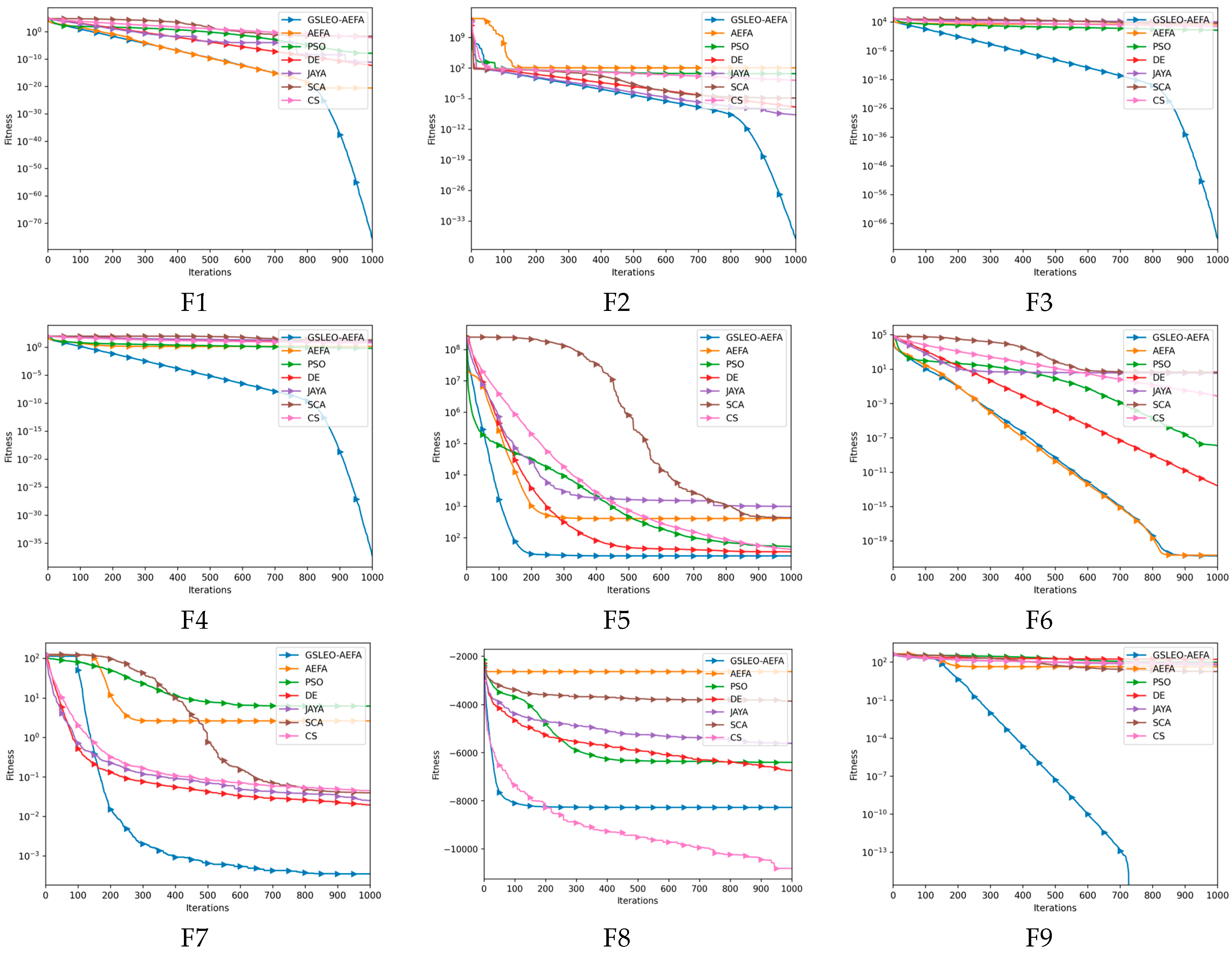
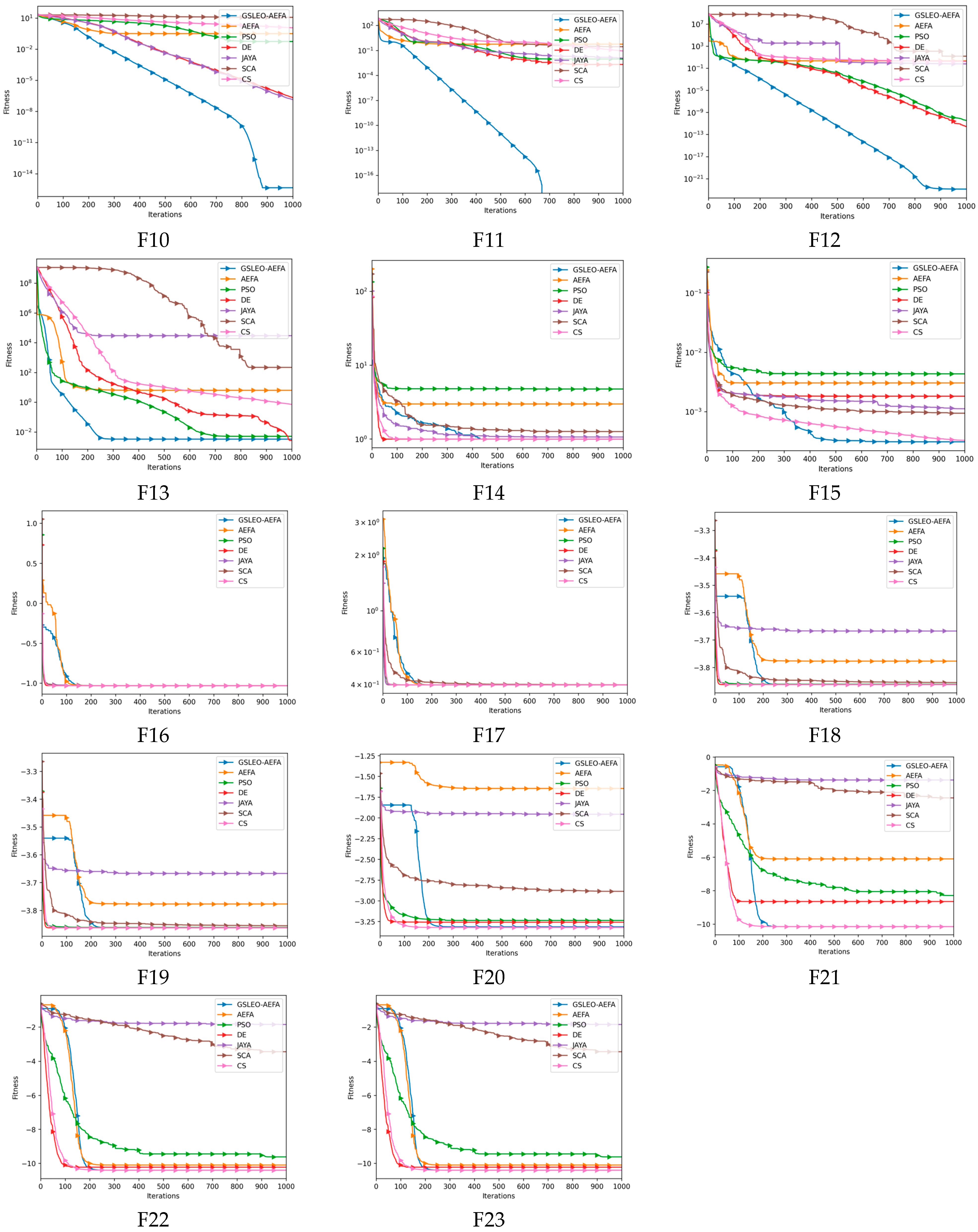
3.2. Convergence Trajectory Analysis

In Figure 4, with F1–F13 set to 30 dimensions, displays the convergence curves of seven different methods. GSLEO-AEFA converged to the global optimum on F9–F11, F16–F17, and F16–F23 and exhibited a greater convergence rate than compared algorithms in multi-modal functions. GSLEO-AEFA significantly increased the convergence accuracy for unimodal functions as compared to the original AEFA (F1–F7). The effective implementation of the LEO mechanism and application of changes to the initial population generation approach ensure that GSLEO-AEFA has enhanced optimization and convergence performance.

3.3. Statistical Test

It is suggested that not only mean and standard deviation comparisons but more evaluation metrics should be used to assess the effectiveness of the metaheuristic algorithms [51]. The use of statistical tests such as the Friedman test and Wilcoxon rank-sum test are advised as effective evaluation metrics to compare the performance of different algorithms.

The significance threshold for the Wilcoxon rank-sum test was set at 0.05. The approach was deemed statistically better, when p < 0.05.

Table 6. Wilcoxon test analysis results.

Dimension	Case	−	+	=	R−	R+	p-Value
30	GSLEO-AEFA vs. AEFA	0	19	4	0	190	1.32 × 10−4
	GSLEO-AEFA vs. PSO	0	19	4	0	190	1.32 × 10−4
	GSLEO-AEFA vs. DE	1	17	5	6	165	5.35 × 10−4
	GSLEO-AEFA vs. JAYA	0	21	2	0	231	6.00 × 10−5
	GSLEO-AEFA vs. SCA	0	20	3	0	210	8.90 × 10−5
	GSLEO-AEFA vs. CS	2	13	8	19	101	1.99 × 10−2
50	GSLEO-AEFA vs. AEFA	0	13	0	0	91	1.32 × 10−4
	GSLEO-AEFA vs. PSO	2	11	0	7	84	1.32 × 10−4
	GSLEO-AEFA vs. DE	1	12	0	7	87	5.35 × 10−4
	GSLEO-AEFA vs. JAYA	0	13	0	0	91	6.00 × 10−5
	GSLEO-AEFA vs. SCA	0	13	0	0	91	8.90 × 10−5
	GSLEO-AEFA vs. CS	1	12	0	12	79	1.99 × 10−2
100	GSLEO-AEFA vs. AEFA	0	13	0	0	91	1.47 × 10−3
	GSLEO-AEFA vs. PSO	0	13	0	0	91	1.47 × 10−3
	GSLEO-AEFA vs. DE	0	13	0	0	91	1.47 × 10−3
	GSLEO-AEFA vs. JAYA	0	13	0	0	91	1.47 × 10−3
	GSLEO-AEFA vs. SCA	0	13	0	0	91	1.47 × 10−3
	GSLEO-AEFA vs. CS	0	13	0	0	91	1.47 × 10−3

displayed the Wilcoxon rank-sum test findings with the notation “+/−/=” denoting whether the recommended approach was superior to, inferior to, or equal to the compared approach [52]. According to Table 6, GSLEO-AEFA always provides R+ values that are greater than R− values. Additionally, Table 6 reveals that the p values of the six algorithms are less than 0.05, indicating that GSLEO-AEFA is superior to the others. The + value of GSLEO-AEFA increased as the dimension increased from 50 to 100, as shown in Table 6. This indicates that the GSLEO-AEFA algorithm performs better than other algorithms, as the dimension increases. The results show that GSLEO-AEFA has higher level of solution accuracy.

The validity of the experiments is evaluated using the Friedman test by contrasting the proposed GSLEO-AEFA with other algorithms. The Friedman test is one of the widely used statistical tests which is used to determine whether more than one techniques’ outputs differ significantly [53]. The outcomes of the Friedman tests are presented in

Table 7. Friedman test for dimension 30, 50, and 100 dimensions for 20 functions.

Test	Dimension	GSLEO-AEFA	AEFA	PSO	DE	JAYA	SCA	CS
Friedman value	30	1.7	4.74	4.3	3.35	5.07	5.33	3.52
Friedman rank		1	5	4	2	6	7	3
Friedman value	50	1.31	5.69	3.31	3.69	4	5.92	4.08
Friedman rank		1	6	2	3	4	7	5
Friedman value	100	1	5.69	3.08	4.62	3.69	5.77	4.15
Friedman rank		1	6	2	5	3	7	4

. The technique that obtains the lowest rank is the most efficient according to Friedman test. In each of the various scenarios, the suggested GSLEO-AEFA is always rated first. Table 7 shows the results for the 30, 50 and 100 dimensions. The GSLEO-AEFA outperforms other algorithms in terms of competitiveness.

In conclusion, AEFA-CSR is more competitive than innovative algorithms such as SCA and CS as well as traditional algorithms such as DE and PSO. The greater accomplishments of GSLEO-AEFA can be attributed to the newly implemented strategies. The LEO solution strategy makes the local optimal escape mechanism better and the GM based SRL makes the population more diversified. As a result, when the two methods are combined, the capacity of GSLEO-AEFA to solve multimodal and unimodal functions is significantly improved.

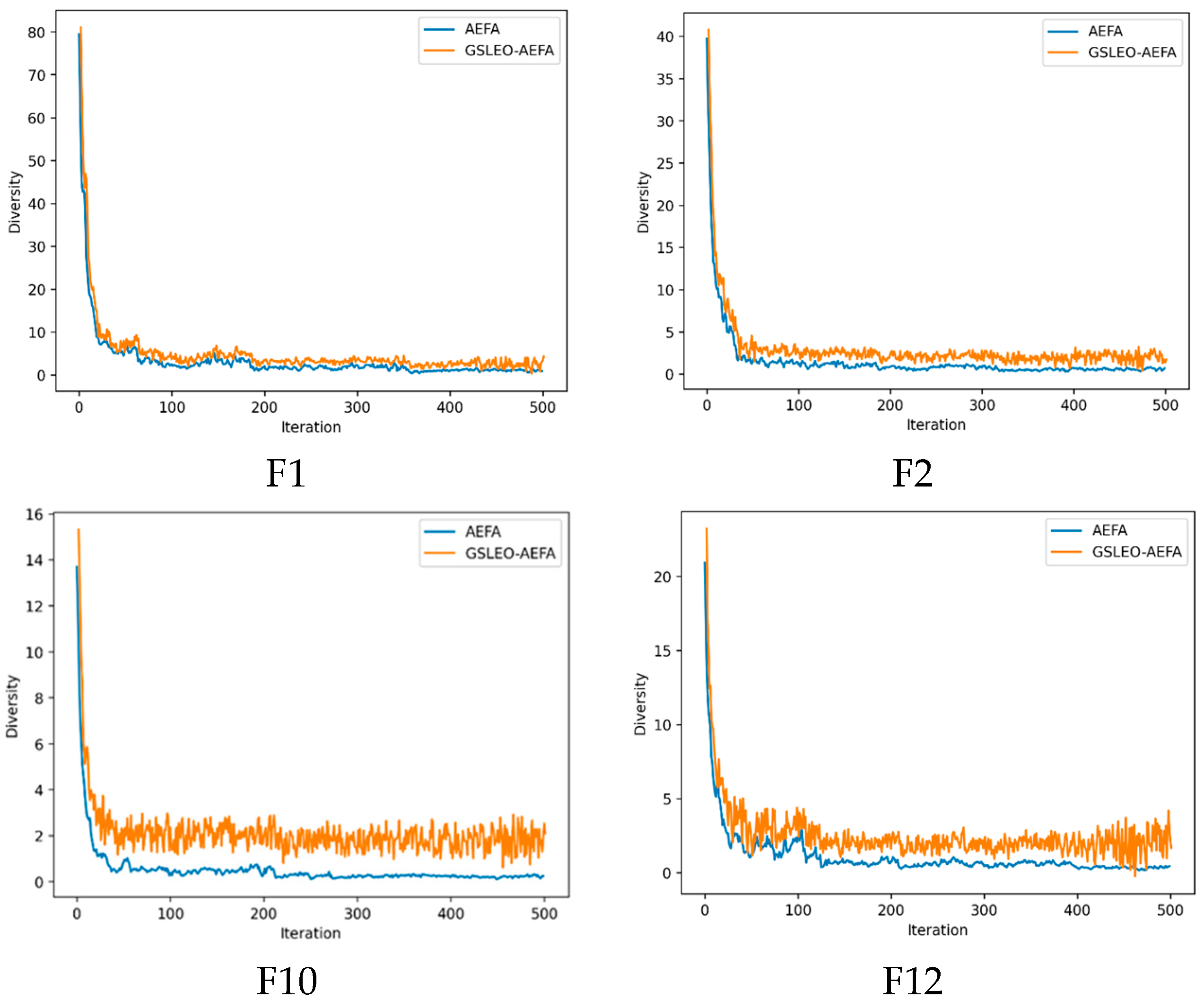
3.4. Diversity Analysis

In order to comprehensively evaluate the performance of the GSLEO-AEFA optimization algorithm, it is imperative to thoroughly investigate the impact of Gaussian mutation and specular reflection on its diversity. To accomplish this, we must calculate the population diversity of both GSLEO-AEFA and AEFA using the following equation [20].

$$\mathit{Diversity}=\frac{1}{N}{{{\displaystyle \sum }}^{}}_{i=1}^N\sqrt{{{{\displaystyle \sum }}^{}}_{j=1}^D}{\left(x_{i,j}-\overline{x_j}\right)}^2,\overline{x_j}=\frac{{{{\displaystyle \sum }}^{}}_{i=1}^N{x}_{i,j}}{N}$$

(36)

Here, D denotes dimension, N represents the number of particles, $x_j$ is jth dimension for the particle at the center of the population and $x_{i,j}$ represents jth dimension of a given particle $i$. To validate the success of GSLEO-AEFA on diversity over the algorithm which is originated from, diversity plots for two unimodal; F1 and F2 and two multimodal; F10 and F12 functions are plotted in Figure 5.

According to the diversity plots for all of the functions analyzed GSLEO-AEFA produces higher diversity than AEFA at each time when it is analyzed. This is an indication of well applied and well suited principles that GSLEO-AEFA contains. Gaussian mutation with local escaping operator successfully enhance the diversification ability of the original algorithm and this is well observed in the plots.

On the other hand, AEFA produces lower diversity and as a result its convergence speed is high. This was expected because of the hybrid nature of the GSLEO-AEFA, since it contains multiple methods to be executed during the optimization.

3.5. Computational Time and Space Complexity Analyses

The total amount of memory used by an algorithm points out the space complexity of that algorithm through the optimization process. The Big O notation of GSLEO-AEFA space complexity can be considered as O (Max_iteration × N × D) where Max_iteration is the number of iterations, N is the number of agents in the population and D is the dimension.

With respect to the computational time, GSLEO-AEFA and the counterpart algorithms are analyzed and the results are shown in

Table 8. Computational time comparison, high values are in bold.

	GSLEO-AEFA	AEFA	PSO	DE	JAYA	SCA	CS
F1	23.990	23.874	40.696	1.801	10.423	10.757	9.059
F2	23.468	23.744	37.481	1.889	10.821	11.391	9.719
F3	30.354	26.628	14.308	4.643	7.535	14.579	15.415
F4	25.580	23.877	11.405	1.593	2.984	10.922	9.229
F5	25.433	24.087	11.716	1.926	3.235	11.538	9.476
F6	32.218	23.863	11.717	1.811	3.135	11.492	9.388
F7	26.256	24.369	12.371	2.109	3.374	11.440	9.427
F8	25.878	24.007	12.553	1.805	3.158	11.541	9.496
F9	25.843	24.081	11.327	1.857	3.075	10.961	9.703
F10	54.693	24.279	12.558	2.208	3.476	11.874	33.917
F11	92.284	24.405	12.796	2.244	3.545	21.765	36.307
F12	90.376	25.107	13.412	3.071	4.267	12.985	37.827
F13	28.186	25.230	13.675	3.263	4.528	12.889	11.843
F14	27.039	15.286	12.312	12.026	10.989	12.206	21.921
F15	8.413	6.382	2.331	1.406	0.968	2.211	2.726
F16	6.080	4.495	0.983	0.740	0.312	0.911	1.224
F17	6.240	4.504	1.017	0.762	0.331	0.947	1.290
F18	6.562	4.608	1.084	0.856	0.414	1.027	1.444
F19	9.443	6.186	2.421	1.785	1.328	2.296	3.366
F20	11.910	8.449	3.723	1.913	1.719	3.529	4.399
F21	17.979	10.459	6.707	5.602	5.251	6.713	10.894
F22	21.677	12.070	8.376	7.261	6.798	8.481	16.520
F23	27.239	14.630	24.862	9.742	9.256	11.081	21.001

. Out of 23 benchmark functions analyzed, for 22 functions, GSLEO-AEFA needs higher CPU time than the others. As a consequence of its hybrid nature, the algorithm GSLEO-AEFA requires more time to figure out the optimization. On the other hand, in terms of precise solutions, GSLEO-AEFA produces high quality results and a researcher may negotiate between the high solution quality and the computational time depending on the problem specifications.

3.6. Overall Discussion

To observe the performance of the newly proposed algorithm GSLEO-AEFA, proper analyses and a set of various experiments were conducted. Considering the original AEFA suffers from the insufficient diversification such powerful tools are added to overcome this issue as well as by allowing the algorithm to escape from local optima and to find solutions that are closer to the global optimum. By achieving this equilibrium between exploration and exploitation, high solution quality is achieved. However, there may be some limitations to consider. Since the proposed algorithm is a hybrid one and formed by multiple methods, the computational time of the algorithm is slightly worse than the other algorithms analyzed. It is because of the running each of the methods during the optimization process, respectively. However, for the ones who consider the precise solution quality, this limitation might be omitted. It is important to consider these factors carefully and to tailor the used of these techniques to the specific problems being solved.

3.7. Engineering Problems

The application of metaheuristics to the solution of engineering problems is one important area of research. In this section, the ability of GSLEO-AEFA to solve engineering problems was evaluated. Four common engineering problems with low and high variables from CLEC 2011 Real World Optimization Problems were used for this test [54]. The evaluation is based on 30 independent runs with 30 populations and a maximum of 1000 iterations. For comparison, the best solution from each optimization algorithm was used.

3.7.1. Parameter Estimation for Frequency-Modulated (FM) Sound Waves

Frequency modulation is a complex multimodal problem. The parameter vector is defined as at $X=\left[a_1,{\omega }_1,a_2,{\omega }_2,a_3,{\omega }_3\right]$ and the fitness function used in the analysis is the sum of the square errors between the estimated wave and the target wave and is given as follows:

$$F(\overrightarrow{X})={{\displaystyle \sum }}_{t=0}^{100}{\left(y\left(t\right)-y_0\left(t\right)\right)}^2$$

(37)

where

$$y\left(t\right)=a_1\cdot \sin \left({\omega }_1\cdot t\cdot \theta +a_2\cdot \sin \left({\omega }_2\cdot t\cdot \theta +a_3\cdot \sin \left({\omega }_3\cdot t\cdot \theta \right)\right)\right)$$

(38)

$$y_0\left(t\right)=\left(1.0\right)\cdot \sin \left(\left(5.0\right)\cdot t\cdot \theta -\left(1.5\right)\cdot \sin \left(\left(4.8\right)\cdot t\cdot \theta +\left(2.0\right)\cdot \sin \left(\left(4.9\right)\cdot t\cdot \theta \right)\right)\right)$$

(39)

The minimum value that needs to be attained is 0. The parameters in the aforementioned equation are defined in the range [−6.4, 6.35] and $\theta$ = $2\pi /100$.

Table 9. Results of parameter estimation for frequency-modulated sound waves.

	GSLEO-AEFA	AEFA	PSO	DE	JAYA	SCA	CS
x(1)	1.00	0.43	−1.00	1.00	−0.63	−1.06	−1.04
x(2)	5.00	0.15	−5.00	5.00	0.00	0.00	−5.02
x(3)	−1.50	2.03	1.50	1.50	4.29	0.69	−1.36
x(4)	4.80	4.98	4.80	−4.80	4.87	0.00	−4.75
x(5)	2.00	0.83	−2.00	−2.00	0.18	−4.45	2.01
x(6)	4.90	−4.41	−4.90	4.90	0.08	−4.88	−4.90
f(x)	0	1.963 × 101	1.950 × 10−27	7.796 × 10−21	1.164 × 101	1.220 × 101	1.888

shows that GSLEO-AEFA discovered superior solution and PSO and DE followed with competitive accuracy. In comparison to other optimizers, GSLEO-AEFA has performed exceptionally well.

3.7.2. Lennard–Jones Potential Problem (LJ)

The Lennard–Jones potential energy minimization problem is a multi-modal optimization problem that involves finding the minimum molecular potential energy of a molecular cluster using the Lennard–Jones potential. The problem has an exponential number of local minima, and the global minima often have structures based on Mackay icosahedrons. The Lennard–Jones potential for $N$ atoms is given by Equation (40), and the optimization algorithm can be used to conform the molecular structure in a way that minimizes energy. To reduce the dimensionality of the problem, one approach is to fix an atom at the origin, choose the second atom to lie on the positive X-axis, and the third atom to lie in the upper half of the X-axis. For each additional atom, three variables (coordinates of the position of the atom) are added to determine the potential energy of the cluster. The variables of the problem have three components for three atoms, six components for four atoms, and so on. The coordinates of each atom are restricted to certain ranges.

Lennard–Jones pair potential for N atoms is given as follows:

$${\overrightarrow{p}}_i=\left\{{\overrightarrow{x}}_i,{\overrightarrow{y}}_i,{\overrightarrow{z}}_i\right\},i=1,\dots ,N$$

(40)

$${\mathrm{V}}_N\left(p\right)={{\displaystyle \sum }}_{i=1}^{N-1}{{\displaystyle \sum }}_{j=i+1}^N\left(r_{ij}^{-12}-2\cdot r_{ij}^{-6}\right)$$

(41)

where $r_{ij}=\Vert {\overrightarrow{p}}_j-{\overrightarrow{p}}_i\Vert {}_2$ with gradient

$${\mathsf{\nabla }}_j{V}_N\left(p\right)=-12{{\displaystyle \sum }}_{i=1,i\ne j}^N\left(r_{ij}^{-14}-r_{ij}^{-8}\right)\left({\overrightarrow{p}}_j-{\overrightarrow{p}}_i\right)$$

(42)

The first decision variable due to the second atom, i.e., $x_1\in \left[0,4\right]$, then the second and third variables are such that $x_2\in \left[0,4\right]$ and $x_3\in \left[0,\pi \right]$. The coordinates $x_i$ for any other atom is taken to be bound in the range; $\left[-4-\frac{1}{4}\left[\frac{i-4}{3}\right],4+\frac{1}{4}\frac{i-4}{3}]\right]$.

The performance results of GSLEO-AEFA and other optimization methods in resolving the Lennard–Jones potential problem are shown in

Table 10. Results Lennard–Jones Potential Problem.

	GSLEO-AEFA	AEFA	PSO	DE	JAYA	SCA	CS
x(1)	0.673	1.338	0.000	0.319	0.551	0.000	2.140
x(2)	0.329	3.307	4.000	0.567	0.035	0.000	2.789
x(3)	0.847	2.115	3.142	1.947	0.745	0.000	1.473
x(4)	0.316	3.639	−4.000	−3.980	−0.237	1.184	0.508
x(5)	−0.608	−3.723	−0.687	3.761	0.661	0.008	−0.682
x(6)	0.884	0.427	4.000	3.855	0.820	0.341	0.722
x(7)	−0.292	0.706	−1.507	−3.970	−0.992	0.337	0.393
x(8)	−0.419	1.807	−3.925	2.768	1.094	−1.074	0.265
x(9)	−0.750	−3.380	−0.706	4.250	0.559	0.005	0.443
x(10)	−0.533	−1.841	−1.260	−4.250	−0.219	−0.909	−1.221
x(11)	0.298	−2.964	−4.109	4.500	0.658	0.382	0.694
x(12)	−0.148	−3.440	0.286	4.453	1.910	−4.500	−1.556
x(13)	0.359	2.205	−1.105	4.500	2.766	0.220	0.327
x(14)	−0.092	2.806	−4.750	−3.053	0.004	0.575	−0.435
x(15)	−0.019	1.921	−1.239	−1.506	−4.750	0.921	−0.238
x(16)	−0.390	2.510	−3.925	−4.357	−0.384	0.172	−2.438
x(17)	−0.681	2.646	−0.770	3.520	0.064	−0.396	0.519
x(18)	0.193	−2.276	5.000	5.000	0.109	0.901	−2.169
x(19)	0.601	0.835	−1.502	−4.099	0.002	0.314	0.090
x(20)	−0.780	3.274	−4.848	5.202	−0.400	−4.879	−1.240
x(21)	−0.879	1.261	−0.337	5.188	1.740	0.073	1.516
x(22)	0.596	−0.687	−3.449	−5.197	0.242	−0.085	0.888
x(23)	−1.042	−0.199	−1.414	4.858	0.795	−0.164	−1.337
x(24)	0.065	3.430	4.400	4.681	−0.010	−0.999	0.042
x(25)	−0.130	0.348	−0.642	−4.883	1.285	−1.179	−1.877
x(26)	−1.369	3.231	−4.341	3.459	0.341	0.350	−0.091
x(27)	−0.494	2.142	−0.456	4.257	0.277	0.044	−1.566
x(28)	−0.289	0.692	−0.814	−3.372	−0.743	−0.659	1.224
x(29)	0.147	4.094	−3.390	5.390	0.003	−0.579	−0.373
x(30)	0.774	1.788	−0.224	4.311	1.361	0.296	0.015
f(x)	−26.027	−7.072	−15.126	−10.615	−14.233	−11.513	−11.646

. The findings make it simple to draw the conclusion that GSLEO-AEFA has superior performance when compared to other algorithms and is capable of solving this issue with high-quality outcomes.

3.7.3. Tersoff Potential Function Minimization Problem (TPF)

Researchers have shown a lot of interest in the evaluation of inter atomic potentials for covalent systems, notably for silicon. One such potential is the Tersoff potential, which controls the interaction of silicon atoms with strong covalent bonding [54]. Two parameterizations of silicon have been provided by Tersoff and are known as Sc (B) and Sc (C). According to the Tersoff formulation, the binding energy is expressed as a sum over atomic sites in the form,

$$E_i=\frac{1}{2}{{\displaystyle \sum }}_{j\ne i}{f}_c\left(r_{ij}\right)\left(V_R\left(r_{ij}\right)-B_{ij}{V}_A\left(r_{ij}\right)\right)$$

(43)

where $V_R$ is a repulsion term, $V_A$ is an attraction term, $f_c\left(r_{ij}\right)$ is a switching function, and $B_{ij}$ is a many-body term that relies on the locations of atoms $i$ and $j$ as well as atom $i$’s neighbors.

$$B_{ij}={\left(1+{\gamma }^{n_1}{\xi }_{ij}^{n_1}\right)}^{-1/2n_1}$$

(44)

$n_1$ and $\gamma$ are standard fitted parameters. For $i$ and $j$ the term ${\xi }_{ij}^{n_1}$ is given as,

$${\xi }_{ij}={{\displaystyle \sum }}_{k\ne i}{f}_c\left(r_{ij}\right)g\left({\theta }_{ijk}\right)\exp \left({\lambda }_3^3{\left(r_{ij}-r_{ik}\right)}^3\right)$$

(45)

The bond angle between $ij$ and $ik$ is denoted as ${\theta }_{ijk}$ which is given as,

$$g\left({\theta }_{ijk}\right)=1+c^2/d^2-c^2/\left(d^2+{\left(h-\cos \left({\theta }_{ijk}\right)\right)}^2\right)$$

(46)

${\lambda }_3$, $c,$ $h$ and $d$ are known as fitted terms. From Equation (41), $V_R$ and $V_A$ are expressed as,

$$V_R\left(r_{ij}\right)=A{e}^{-{\lambda }_1{r}_{ij}}$$

(47)

$$V_A\left(r_{ij}\right)=B{e}^{-{\lambda }_2{r}_{ij}}$$

(48)

Expressed as fitted parameters are $A$, $B$, ${\lambda }_1$ and ${\lambda }_2$. In Equation (43), the switching function $f_c\left(r_{ij}\right)$ is expressed as,

$$f_c\left(r_{ij}\right)=\{\begin{array}{c}1\\ \frac{1}{2}-\frac{1}{2}\sin \left[\frac{\pi \left(r_{ij}-R\right)}{D}\right]\\ 0\end{array}\begin{array}{c}if r_{ij}<R-D\\ if R-D<r_{ij}<R+D\\ if r_{ij}\ge R+D\end{array}$$

(49)

We must determine the energy of each atom in order to determine the minimal potential energy for atoms. Each atom, let us say atom $i$ has a unique potential energy, $E_i$, which is determined by Equation (43). Therefore, in order to compute Equation (43), which requires the computation of Equations (44)–(49) for each neighbor of that atom, to know the potential energy of a single atom.

Similar to the Lennard–Jones potential problem, the first decision variable due to the second atom, i.e., $x_1\in \left[0,4\right]$, then the second and third variables are such that $x_2\in \left[0,4\right]$ and $x_3\in \left[0,\pi \right]$. The coordinates $x_i$ for any other atom is taken to be bound in the range; $\left[-4-\frac{1}{4}\left[\frac{i-4}{3}\right],4+\frac{1}{4}\frac{i-4}{3}]\right]$.

Table 11. Results of Tersoff Potential Function Minimization Problem.

	GSLEO-AEFA	AEFA	PSO	DE	JAYA	SCA	CS
x(1)	0.000	2.497	1.984	3.427	1.135	4.000	1.613
x(2)	4.000	1.998	2.758	3.992	3.908	0.000	0.041
x(3)	3.142	2.318	2.274	0.482	0.544	0.000	1.485
x(4)	−1.000	3.773	−0.367	−1.000	−1.000	−0.643	2.922
x(5)	−1.000	−0.847	2.762	−0.564	2.594	1.112	1.791
x(6)	3.708	2.595	2.675	1.612	1.478	0.203	3.856
x(7)	2.029	1.302	1.293	−0.282	0.650	−0.004	2.913
x(8)	3.931	4.107	−0.081	4.250	−0.336	4.250	4.246
x(9)	4.250	1.767	3.521	−1.000	1.907	0.869	−0.678
x(10)	4.250	1.168	2.749	4.250	3.417	0.378	2.498
x(11)	0.988	3.042	4.337	2.937	−0.068	−1.000	1.256
x(12)	−1.000	−0.259	0.648	4.500	0.543	−0.008	−0.216
x(13)	−0.252	3.947	2.291	4.500	0.733	2.123	2.467
x(14)	0.925	−0.869	−0.738	0.681	3.206	4.536	3.973
x(15)	4.750	0.265	1.450	3.802	2.760	0.635	3.515
x(16)	1.140	3.452	3.454	0.258	4.672	1.995	0.205
x(17)	−0.914	3.721	−1.000	1.553	−1.000	0.314	0.707
x(18)	4.581	1.334	3.504	2.542	−1.000	1.082	−0.223
x(19)	5.000	2.934	0.756	1.062	−0.443	0.957	1.043
x(20)	−1.000	4.288	4.810	0.250	5.148	0.865	2.234
x(21)	−0.085	−0.324	1.972	1.091	2.056	4.665	1.313
x(22)	0.438	1.828	4.238	−1.000	5.167	1.721	0.115
x(23)	5.500	−0.530	0.585	1.432	1.281	3.192	−0.580
x(24)	4.847	−0.955	1.934	0.299	−0.048	−0.799	4.081
x(25)	1.548	5.123	3.034	3.795	−0.393	−0.054	3.977
x(26)	5.689	1.252	4.830	2.514	−1.000	−0.474	2.986
x(27)	2.827	2.750	2.998	2.063	−0.757	2.376	1.977
x(28)	−0.686	4.798	1.078	1.325	5.491	−1.000	4.752
x(29)	−0.972	4.188	3.857	2.934	−0.865	−0.077	3.163
x(30)	6.000	4.687	4.240	−1.000	1.094	4.160	4.110
f(x)	−34.108	−14.888	−30.559	−24.606	−31.065	−20.620	−31.737

of the test results for the TPF demonstrates that GSLEO-AEFA outperformed other optimizers and was able to offer a significantly superior solution. Additionally, it has performed effectively as engineering issues have become more constrained.

3.7.4. Antenna Optimization Problem

Zhang et al. suggested a validated a benchmark test suite for Antenna S-parameter optimization [55]. In the test suite there are unimodal, multimodal, and compositional functions. Each of these functions matches a typical landscape of electromagnetic simulated antenna problems. For this analysis two functions were chosen which can approximate the s-parameter optimization function behavior of two different antennas. Equations (50) and (51) model the single antenna and multi-antenna problems, respectively. Function in Equation (50) is continuous and separable and the landscape has a rose shape which is similar to the patterns of the dual band antenna. Function in Equation (51) is continuous non-differentiable and non-separable and its landscape is similar to the reflection pattern of the (multiple input–multiple output) MIMO antenna.

$$s_1\left(x\right)=20\log \left(2\left({{\displaystyle \sum }}_{i=1}^n\left|{\left(\sin \left(\frac{x_i}{8}\right)\right)}^2\right|+{{\displaystyle \prod }}_{i=1}^n\left|\sin \left(\frac{x_i}{8}\right)\right|\right)+1\right)$$

(50)

$$\begin{gathered} \begin{array}{c}{s}_2\left(x\right)=100\sqrt{\left|x_2+1-0.01{\left(x_1-10\right)}^2\right|}+0.01\left|x_1\right|\end{array}+ \\ 20\log \left(0.01{\left({{\displaystyle \sum }}_{i=1}^n\left|x_i\right|\right)}^2{\left(\sin \left(0.8x_1\right)+2\right)}^4+1\right) \end{gathered}$$

(51)

We evaluated GSLEO-AEFA and its counterpart algorithms with a population size of 30, iteration of 500 and a dimension set to 8, as recommended by Zhang et al. [55], by considering that the s-parameters of most antennas are around 10. The performance of each algorithm after 30 independent runs in Table 11, using average and standard deviation metrics are recorded. Our analysis indicates that GSLEO-AEFA provided the best results for both single-antenna and multi-antenna problems by demonstrating its effectiveness in solving complex optimization problems in this domain, as seen in

Table 12. Results of antenna S-parameter optimization problem, significant values are in bold.

		GSLEO-AEFA	AEFA	PSO	DE	JAYA	SCA	CS
s1	AVG	0.000	1.351	1.083 × 10−2	1.603	5.448	1.370 × 101	5.477
	STD	0.000	2.469 × 10−1	5.946 × 10−4	2.752 × 10−1	4.379	1.915	5.862 × 10−1
s2	AVG	8.611 × 10−7	6.839 × 101	7.255 × 101	3.407 × 101	9.047 × 101	8.684 × 101	8.040 × 101
	STD	1.756 × 10−6	9.564	4.589	5.161	1.687 × 10+1	1.192 × 101	3.057

.

To observe the performance of the newly proposed algorithm GSLEO-AEFA, proper analyses and a set of various experiments were conducted. Considering the original AEFA suffers from the insufficient diversification such powerful tools are added to overcome this issue as well as by allowing the algorithm to escape from local optima and to find solutions that are closer to the global optimum. By achieving this equilibrium between exploration and exploitation, high solution quality is achieved. However, there may be some limitations to consider. Since the proposed algorithm is a hybrid one and formed by multiple methods, the computational time of the algorithm is slightly worse than the other algorithms analyzed. It is because of running each of the methods during the optimization process, respectively. However, for the ones who consider the precise solution quality, this limitation might be omitted. It is important to consider these factors carefully and to tailor the used of these techniques to the specific problems being solved.

4. Conclusions

The performance of the proposed methodology GSLEO-AEFA with its counterpart algorithms were tested on 23 benchmark functions by conducting overall effectiveness, convergence analysis, Friedman and Wilcoxon rank-sum statistical tests as well as computational analysis. Even in the varying dimension sizes, GSLEO-AEFA has achieved the best optimization accuracy among the algorithms tested.

The performance of GSLEO-AEFA was then validated on real engineering design problems including antenna optimization. In here, it has been outlined that the success of the proposed algorithm was maintained at the same level for all of the design problems. The proper use of local escaping operator (LEO), Gaussian mutation (GM) and specular reflection learning (SRL) techniques in the algorithm GSLEO-AEFA provides a better balance in exploration and exploitation by overcoming not only the original algorithm which is derived from but the other algorithms used in the comparison.

Although its performance is quite satisfactory, it can be acknowledged that the computational time is not always satisfactory. This is mainly caused because of the structure of the GSLEO-AEFA, since it was generated by having three individual methods as well as AEFA. However, researchers may debate for a fine balance between the optimization accuracy and the computational time for the problem to be solved.

References

1. Mahariq, I. On the application of the spectral element method in electromagnetic problems involving domain decomposition. Turk. J. Electr. Eng. Comput. Sci. 2017, 25, 1059–1069. [Google Scholar] [CrossRef]
2. Yang, C.X.; Zhang, J.; Tong, M.S. A Hybrid Quantum-Behaved Particle Swarm Optimization Algorithm for Solving Inverse Scattering Problems. IEEE Trans. Antennas Propag. 2021, 69, 5861–5869. [Google Scholar] [CrossRef]
3. Donelli, M.; Franceschini, D.; Rocca, P.; Massa, A. Three-Dimensional Microwave Imaging Problems Solved Through an Efficient Multiscaling Particle Swarm Optimization. IEEE Trans. Geosci. Remote Sens. 2009, 47, 1467–1481. [Google Scholar] [CrossRef]
4. Gupta, S.; Deep, K. A memory-based Grey Wolf Optimizer for global optimization tasks. Appl. Soft Comput. 2020, 93, 106367. [Google Scholar] [CrossRef]
5. Kennedy, J.; Eberhart, R. Particle swarm optimization. In Proceedings of the ICNN’95-International Conference on Neural Networks, Perth, WA, Australia, 27 November–1 December 1995; Volume 4, pp. 1942–1948. [Google Scholar]
6. Abbas, M.; Alshehri, M.A.; Barnawi, A.B. Potential Contribution of the Grey Wolf Optimization Algorithm in Reducing Active Power Losses in Electrical Power Systems. Appl. Sci. 2022, 12, 6177. [Google Scholar] [CrossRef]
7. El Gmili, N.; Mjahed, M.; El Kari, A.; Ayad, H. Particle Swarm Optimization and Cuckoo Search-Based Approaches for Quadrotor Control and Trajectory Tracking. Appl. Sci. 2019, 9, 1719. [Google Scholar] [CrossRef] [Green Version]
8. Li, Y.; Pei, Y.-H.; Liu, J.-S. Bat optimal algorithm combined uniform mutation with Gaussian mutation. Kongzhi Yu Juece/Control Decis. 2017, 32, 1775–1781. [Google Scholar] [CrossRef]
9. Yuan, X.; Miao, Z.; Liu, Z.; Yan, Z.; Zhou, F. Multi-Strategy Ensemble Whale Optimization Algorithm and Its Application to Analog Circuits Intelligent Fault Diagnosis. Appl. Sci. 2020, 10, 3667. [Google Scholar] [CrossRef]
10. Ni, J.; Tang, J.; Wang, R. Hybrid Algorithm of Improved Beetle Antenna Search and Artificial Fish Swarm. Appl. Sci. 2022, 12, 13044. [Google Scholar] [CrossRef]
11. Sun, L.; Feng, B.; Chen, T.; Zhao, D.; Xin, Y. Equalized Grey Wolf Optimizer with Refraction Opposite Learning. Comput. Intell. Neurosci. 2022, 2022, e2721490. [Google Scholar] [CrossRef]
12. David, R.-C.; Precup, R.-E.; Petriu, E.M.; Rădac, M.-B.; Preitl, S. Gravitational search algorithm-based design of fuzzy control systems with a reduced parametric sensitivity. Inf. Sci. 2013, 247, 154–173. [Google Scholar] [CrossRef]
13. Mirjalili, S. SCA: A Sine Cosine Algorithm for solving optimization problems. Knowl.-Based Syst. 2016, 96, 120–133. [Google Scholar] [CrossRef]
14. Kaveh, A.; Mahdavi, V.R. Colliding Bodies Optimization method for optimum discrete design of truss structures. Comput. Struct. 2014, 139, 43–53. [Google Scholar] [CrossRef]
15. Zheng, H.; Gao, J.; Xiong, J.; Yao, G.; Cui, H.; Zhang, L. An Enhanced Artificial Electric Field Algorithm with Sine Cosine Mechanism for Logistics Distribution Vehicle Routing. Appl. Sci. 2022, 12, 6240. [Google Scholar] [CrossRef]
16. Juárez-Pérez, F.; Cruz-Chávez, M.A.; Rivera-López, R.; Ávila-Melgar, E.Y.; Eraña-Díaz, M.L.; Cruz-Rosales, M.H. Grid-Based Hybrid Genetic Approach to Relaxed Flexible Flow Shop with Sequence-Dependent Setup Times. Appl. Sci. 2022, 12, 607. [Google Scholar] [CrossRef]
17. Wang, S.L.; Adnan, S.H.; Ibrahim, H.; Ng, T.F.; Rajendran, P. A Hybrid of Fully Informed Particle Swarm and Self-Adaptive Differential Evolution for Global Optimization. Appl. Sci. 2022, 12, 11367. [Google Scholar] [CrossRef]
18. Eltaeib, T.; Mahmood, A. Differential Evolution: A Survey and Analysis. Appl. Sci. 2018, 8, 1945. [Google Scholar] [CrossRef] [Green Version]
19. Fogel, G.B. Evolutionary Programming. In Handbook of Natural Computing; Rozenberg, G., Bäck, T., Kok, J.N., Eds.; Springer: Berlin, Heidelberg, 2012; pp. 699–708. ISBN 978-3-540-92910-9. [Google Scholar]
20. Liu, X.; Wang, Y.; Zhou, M. Dimensional Learning Strategy-Based Grey Wolf Optimizer for Solving the Global Optimization Problem. Comput. Intell. Neurosci. 2022, 2022, 3603607. [Google Scholar] [CrossRef]
21. Črepinšek, M.; Liu, S.-H.; Mernik, M. Exploration and exploitation in evolutionary algorithms: A survey. ACM Comput. Surv. 2013, 45, 35:1–35:33. [Google Scholar] [CrossRef]
22. Anita; Yadav, A. AEFA: Artificial electric field algorithm for global optimization. Swarm Evol. Comput. 2019, 48, 93–108. [Google Scholar] [CrossRef]
23. Sinthia, P.; Malathi, M. Cancer detection using convolutional neural network optimized by multistrategy artificial electric field algorithm. Int. J. Imaging Syst. Technol. 2021, 31, 1386–1403. [Google Scholar] [CrossRef]
24. Petwal, H.; Rani, R. An Improved Artificial Electric Field Algorithm for Multi-Objective Optimization. Processes 2020, 8, 584. [Google Scholar] [CrossRef]
25. Selem, S.I.; El-Fergany, A.A.; Hasanien, H.M. Artificial electric field algorithm to extract nine parameters of triple-diode photovoltaic model. Int. J. Energy Res. 2021, 45, 590–604. [Google Scholar] [CrossRef]
26. Niroomand, S. Hybrid artificial electric field algorithm for assembly line balancing problem with equipment model selection possibility. Knowl.-Based Syst. 2021, 219, 106905. [Google Scholar] [CrossRef]
27. Das, H.; Naik, B.; Behera, H.S. Optimal Selection of Features Using Artificial Electric Field Algorithm for Classification. Arab. J. Sci. Eng. 2021, 46, 8355–8369. [Google Scholar] [CrossRef]
28. Houssein, E.H.; Hashim, F.A.; Ferahtia, S.; Rezk, H. An efficient modified artificial electric field algorithm for solving optimization problems and parameter estimation of fuel cell. Int. J. Energy Res. 2021, 45, 20199–20218. [Google Scholar] [CrossRef]
29. Bi, J.; Zhou, Y.; Tang, Z.; Luo, Q. Artificial electric field algorithm with inertia and repulsion for spherical minimum spanning tree. Appl. Intell. 2022, 52, 195–214. [Google Scholar] [CrossRef]
30. Alanazi, A.; Alanazi, M. Artificial Electric Field Algorithm-Pattern Search for Many-Criteria Networks Reconfiguration Considering Power Quality and Energy Not Supplied. Energies 2022, 15, 5269. [Google Scholar] [CrossRef]
31. Cheng, J.; Xu, P.; Xiong, Y. An improved artificial electric field algorithm and its application in neural network optimization. Comput. Electr. Eng. 2022, 101, 108111. [Google Scholar] [CrossRef]
32. Malisetti, N.; Pamula, V.K. Energy efficient cluster based routing for wireless sensor networks using moth levy adopted artificial electric field algorithm and customized grey wolf optimization algorithm. Microprocess. Microsyst. 2022, 93, 104593. [Google Scholar] [CrossRef]
33. Nayak, S.C.; Sanjeev Kumar Dash, C.; Behera, A.K.; Dehuri, S. An Elitist Artificial-Electric-Field-Algorithm-Based Artificial Neural Network for Financial Time Series Forecasting. In Biologically Inspired Techniques in Many Criteria Decision Making; Dehuri, S., Prasad Mishra, B.S., Mallick, P.K., Cho, S.-B., Eds.; Springer Nature: Singapore, 2022; pp. 29–38. [Google Scholar]
34. Rahnamayan, S.; Tizhoosh, H.R.; Salama, M.M.A. Opposition-Based Differential Evolution. IEEE Trans. Evol. Comput. 2008, 12, 64–79. [Google Scholar] [CrossRef] [Green Version]
35. Zhang, Y. Backtracking search algorithm with specular reflection learning for global optimization. Knowl.-Based Syst. 2021, 212, 106546. [Google Scholar] [CrossRef]
36. Alkayem, N.F.; Shen, L.; Al-hababi, T.; Qian, X.; Cao, M. Inverse Analysis of Structural Damage Based on the Modal Kinetic and Strain Energies with the Novel Oppositional Unified Particle Swarm Gradient-Based Optimizer. Appl. Sci. 2022, 12, 11689. [Google Scholar] [CrossRef]
37. Alkayem, N.F.; Shen, L.; Asteris, P.G.; Sokol, M.; Xin, Z.; Cao, M. A new self-adaptive quasi-oppositional stochastic fractal search for the inverse problem of structural damage assessment. Alex. Eng. J. 2022, 61, 1922–1936. [Google Scholar] [CrossRef]
38. Adegboye, O.R.; Ülker, E.D. A Quick Performance Assessment for Artificial Electric Field Algorithm. In Proceedings of the 2022 International Congress on Human-Computer Interaction, Optimization and Robotic Applications (HORA), Ankara, Turkey, 9–11 June 2022; pp. 1–5. [Google Scholar]
39. Sajwan, A.; Yadav, A. A study of exploratory and stability analysis of artificial electric field algorithm. Appl. Intell. 2022, 52, 10805–10828. [Google Scholar] [CrossRef]
40. Yang, W.; Xia, K.; Li, T.; Xie, M.; Zhao, Y. An Improved Transient Search Optimization with Neighborhood Dimensional Learning for Global Optimization Problems. Symmetry 2021, 13, 244. [Google Scholar] [CrossRef]
41. Liu, Y.; Heidari, A.A.; Cai, Z.; Liang, G.; Chen, H.; Pan, Z.; Alsufyani, A.; Bourouis, S. Simulated annealing-based dynamic step shuffled frog leaping algorithm: Optimal performance design and feature selection. Neurocomputing 2022, 503, 325–362. [Google Scholar] [CrossRef]
42. Dai, M.; Feng, X.; Yu, H.; Guo, W. An opposition-based differential evolution clustering algorithm for emotional preference and migratory behavior optimization. Knowl.-Based Syst. 2023, 259, 110073. [Google Scholar] [CrossRef]
43. Nama, S.; Saha, A.K.; Sharma, S. Performance up-gradation of Symbiotic Organisms Search by Backtracking Search Algorithm. J Ambient. Intell Hum. Comput. 2022, 13, 5505–5546. [Google Scholar] [CrossRef]
44. Duan, Y.; Liu, C.; Li, S.; Guo, X.; Yang, C. Gaussian Perturbation Specular Reflection Learning and Golden-Sine-Mechanism-Based Elephant Herding Optimization for Global Optimization Problems. Comput. Intell. Neurosci. 2021, 2021, e9922192. [Google Scholar] [CrossRef]
45. Emambocus, B.A.S.; Jasser, M.B.; Mustapha, A.; Amphawan, A. Dragonfly Algorithm and Its Hybrids: A Survey on Performance, Objectives and Applications. Sensors 2021, 21, 7542. [Google Scholar] [CrossRef]
46. Ahmadianfar, I.; Bozorg-Haddad, O.; Chu, X. Gradient-based optimizer: A new metaheuristic optimization algorithm. Inf. Sci. 2020, 540, 131–159. [Google Scholar] [CrossRef]
47. Storn, R.; Price, K. Differential Evolution–A Simple and Efficient Heuristic for global Optimization over Continuous Spaces. J. Glob. Optim. 1997, 11, 341–359. [Google Scholar] [CrossRef]
48. Venkata Rao, R. Jaya: A simple and new optimization algorithm for solving constrained and unconstrained optimization problems. Int. J. Ind. Eng. Comput. 2016, 7, 19–34. [Google Scholar] [CrossRef]
49. Yang, X.-S.; Deb, S. Cuckoo Search via Lévy flights. In Proceedings of the 2009 World Congress on Nature & Biologically Inspired Computing (NaBIC), Coimbatore, India, 9–11 December 2009; pp. 210–214. [Google Scholar]
50. Qaraad, M.; Amjad, S.; Hussein, N.K.; Mirjalili, S.; Halima, N.B.; Elhosseini, M.A. Comparing SSALEO as a Scalable Large Scale Global Optimization Algorithm to High-Performance Algorithms for Real-World Constrained Optimization Benchmark. IEEE Access 2022, 10, 95658–95700. [Google Scholar] [CrossRef]
51. García, S.; Molina, D.; Lozano, M.; Herrera, F. A study on the use of non-parametric tests for analyzing the evolutionary algorithms’ behaviour: A case study on the CEC’2005 Special Session on Real Parameter Optimization. J. Heuristics 2008, 15, 617. [Google Scholar] [CrossRef]
52. Derrac, J.; García, S.; Molina, D.; Herrera, F. A practical tutorial on the use of nonparametric statistical tests as a methodology for comparing evolutionary and swarm intelligence algorithms. Swarm Evol. Comput. 2011, 1, 3–18. [Google Scholar] [CrossRef]
53. Zamani, H.; Nadimi-Shahraki, M.H.; Gandomi, A.H. CCSA: Conscious Neighborhood-based Crow Search Algorithm for Solving Global Optimization Problems. Appl. Soft Comput. 2019, 85, 105583. [Google Scholar] [CrossRef]
54. Swagatam, D.; Suganthan, P.N. Problem Definitions and Evaluation Criteria for CEC 2011 Competition on Testing Evolutionary Algorithms on Real World Optimization Problems; Jadavpur University, Nanyang Technological University: Kolkata, India, 2011. [Google Scholar]
55. Zhang, Z.; Chen, H.; Jiang, F.; Yu, Y.; Cheng, Q.S. A Benchmark Test Suite for Antenna S-Parameter Optimization. IEEE Trans. Antennas Propagat. 2021, 69, 6635–6650. [Google Scholar] [CrossRef]
Figure 1. Illustration of the forces exerted on charges.
Applsci 13 04157 g001
Figure 2. Specular reflection learning illustration; (a) The phenomenon of specular reflection and (b) The model of specular reflection.
Applsci 13 04157 g002
Figure 3. Flowchart of GSLEO-AEFA.
Applsci 13 04157 g003
Figure 4. Convergence trajectory graphs for all studied benchmark functions F1–F23.
Applsci 13 04157 g004aApplsci 13 04157 g004b
Figure 5. Diversity plots for GSLEO-AEFA and AEFA for the unimodal functions F1, F2 and the multimodal functions F10, F12.
Applsci 13 04157 g005