Qualitative and Quantitative Evaluation of Multivariate Time-Series Synthetic Data Generated Using MTS-TGAN: A Novel Approach

Abstract

To obtain high performance, generalization, and accuracy in machine learning applications, such as prediction or anomaly detection, large datasets are a necessary prerequisite. Moreover, the collection of data is time-consuming, difficult, and expensive for many imbalanced or small datasets. These challenges are evident in collecting data for financial and banking services, pharmaceuticals and healthcare, manufacturing and the automobile, robotics car, sensor time-series data, and many more. To overcome the challenges of data collection, researchers in many domains are becoming more and more interested in the development or generation of synthetic data. Generating synthetic time-series data is far more complicated and expensive than generating synthetic tabular data. The primary objective of the paper is to generate multivariate time-series data (for continuous and mixed parameters) that are comparable and evaluated with real multivariate time-series synthetic data. After being trained to produce such data, a novel GAN architecture named as MTS-TGAN is proposed and then assessed using both qualitative measures namely t-SNE, PCA, discriminative and predictive scores as well as quantitative measures, for which an RNN model is implemented, which calculates MAE and MSLE scores for three training phases; Train Real Test Real, Train Real Test Synthetic and Train Synthetic Test Real. The model is able to reduce the overall error up to 13% and 10% in predictive and discriminative scores, respectively. The research’s objectives are met, and the outcomes demonstrate that MTS-TGAN is able to pick up on the distribution and underlying knowledge included in the attributes of the real data and it can serve as a starting point for additional research in the respective area.

1. Introduction

One of today’s most vital resources is data. However, they are expensive, sensitive, take time to process, and are either unavailable or need to be kept confidential due to personally identifiable information (PII) or compliance problems [1]. Any disclosure or sharing of personally identifiable consumer information may result in expensive legal actions that also harm the reputation of the organization. Additionally, data are typically not accessible for relatively new works [2]. Additionally, the process of the human annotation of data is expensive and time-consuming. Therefore, reducing privacy issues and opting for an economical option is the main justification for why businesses invest in synthetic data-generating techniques. Information that has been intentionally annotated is known as synthetic data. It is produced via simulations or computer algorithms.

Businesses can benefit from synthetic data for three primary reasons: they can be used to train machine learning algorithms, they can be used to test products more quickly, and they can help with privacy issues. The majority of data privacy regulations impose limitations on how sensitive data are handled by organizations [2]. When training artificial intelligent (AI) models, developers frequently need huge datasets with precise labeling. As when trained on a wider variety of data, neural networks become more accurate. Collecting and labeling these massive datasets containing hundreds or even millions of objects or information, however, can be unreasonably time and money-consuming, as well as labor-intensive. For these reasons, the generation of synthetic data is crucial. Some areas which have an application of synthetic data are as follows:

• Financial and banking services.
• Pharmaceuticals and healthcare.
• Manufacturing and automobiles.
• Robotics.
• Digital marketing and internet advertising.
• Espionage and security businesses.

There are different types of data that can be synthesized, such as tabular data, image, video data, sound data, and time-series data. However, creating synthetic time-series data is far trickier than creating synthetic tabular data [3]. The primary distinction is that real tabular data assume that each row of the data contains information on a single person, whereas time-sensitive data, on the other hand, is dispersed across numerous columns and rows in various time sequences or frames. The difficulty of this task is also influenced by the duration of the time-series data; the longer the history, the more challenging it is to learn the features of the original and generated synthetic data from it.

Generative adversarial network models (GANs) [4] can supplement smaller datasets by producing new and unused data. In some circumstances, data may be corrupted, distorted, or missing. GANs can impute data, or substitute the anomalies with information corresponding to clean data. In the case of corrupted data, they can also denoise signals. Data security, privacy, and sharing are now severely controlled; they can add an additional degree of protection by creating differentially private datasets that do not run the danger of being linked to their source data [5].

GANs [4] has become a well-liked way for creating or enhancing datasets, particularly with images and videos. However, when it comes to networking data, which includes both mixed discrete, continuous, and intricate temporal correlation data types, GANs perform poorly [6]. Even while GAN-based time-series generation is possible, for example, for medical time series, these methods fall short for more complicated data, showing low autocorrelation scores on lengthy sequences and being vulnerable to mode collapse [5].

Sensor readings, time-stamped log messages, stock market values, and medical records are a few examples of the potential uses for synthetic time-series data. Synthetic data face numerous difficulties because of the additional dimension of time, where trends and correlations across time are just as significant as correlations between variables [7]. To overcome this, TimeGAN (time-series generative adversarial network) [8] was introduced, but still, the multivariate factor was not properly addressed, and further increasing the number of parameters and size, it was unable to perform adequately.

Unfortunately, there is no set consensus on the metrics for evaluating the generated data for time-series GANs because of the small number of research studies that have been published [9,10,11,12]. Different strategies [13,14] have been put out, but as of now, none has emerged as the leader in the metrics field. Hence, we, in this research, have aimed at improving the time-series (TS) data’s multivariate factor by implementing our proposed model named MTS-TGAN, which is an extension of TimeGAN [8]. The novelty of the paper is designing, implementing, and evaluating (both qualitatively and quantitatively) the model which can generate multivariate time-series data with better evaluation scores. The further novelty of our proposed model (MTS-TGAN) includes the inception of a pre-processing layer, namely, a feature selector which outputs the important features that help in removing extra noise, which hinders the synthetic generation of data, as well as hyper-parameter tuning, such as having a number of GRU layers [15], such as six (for all four modules, namely generator (G), discriminator (D), embedding (E) and recovery (R) functions) [8] and using the activation function ReLU [16] and implementing the proposed model on two datasets, such as a Google stock [17] and UniMiB human activity recognition (HAR) dataset [18] to show that the model is efficient in working with the multivariate TS data.

An outline of the paper is as follows: In Section 2, related research in this field is compared and contrasted. Section 3 presents the problem statement. Section 4 discusses the proposed MTS-TGAN model. By summarizing the experimentation’s outcomes, Section 5 provides a summary of the main findings. Section 6 provides the conclusions and suggests potential directions for additional research.

2. Related Works

Numerous research studies, including Refs. [19,20,21,22,23], have been conducted since the GAN framework was first introduced in 2014 by Goodfellow et al. [4], which consists of two neural networks (NN) models, typically, a generator G and a discriminator D. GANs have gained a lot of attention among deep learning (DL) researchers, but the majority of the experiments were concerned with the creation of images such as creating anime characters [19], creating photos of people’s faces [20], image in-painting [21], creating bedroom images [22], and removing noise (rain) from images [23]. Their success is partly due to their capacity for producing and modifying data across several fields. While computer vision (CV) has been the primary use for GANs up to this point, they have also been successfully used in other contexts, such as natural language processing (NLP). GANs have recently shown that they are capable of generating high-quality images and videos as well as style transfer and image completeness [20,22,23]. 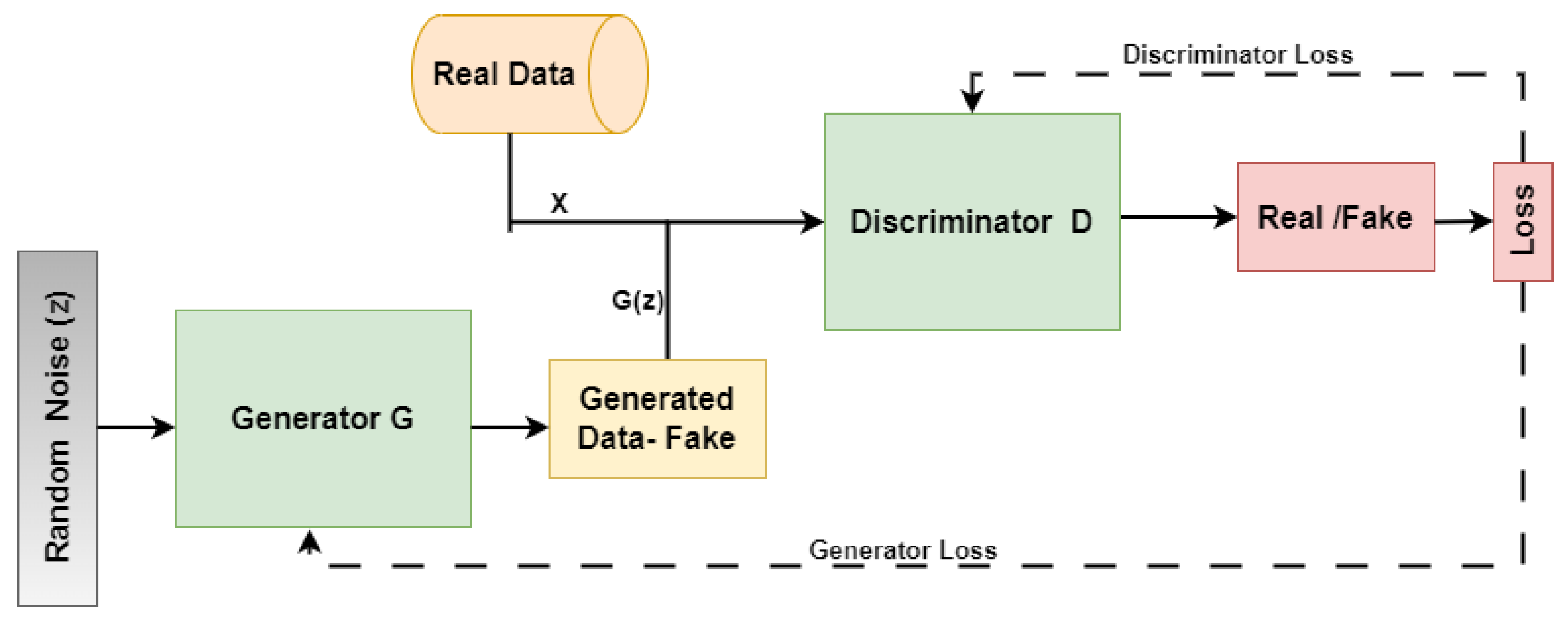Additionally, they have been utilized with effectiveness for imputation, sequence predicting, and audio generation as shown in Figure 1.

A trend has emerged toward the production of time-series and sequential data using GANs, as well as forecasting. However, research on using GANs to generate time-series has not been as thorough. Here are few papers [8,24,25,26,27,28,29,30] that implemented GANs using time-series data as per our knowledge, which is discussed further in this Section.

Mogren et al. [24] carried out one of the earliest research on time-series generation using GANs. In this study, an adversarial training continuous recurrent neural network model for music generation was proposed. The author acknowledged that their approach still requires improvement, particularly in terms of a rigorous assessment of the generated data’s quality.

Time-conditional GAN is a new GAN framework that Ramponi et al. [25] proposed at the beginning of 2019. Its generator and discriminator are both conditioned on the sampling timestamps. The goal of their effort was to identify a time-series data-augmentation technique. They contrasted their model against two very straightforward methods, time slicing and time warping [31]. They carried out a classification task as an evaluation, and they achieved improved classification accuracy using their suggested model.

The model is intended to support end users’ decision-making processes, particularly with regard to financial portfolio decisions. On structured decision-related quantities, it employs a multi-Wasserstein loss [32] by Hao et al. [26]. Sun et al. [27] implemented DAT-CGAN, in which each input, which in this case is assets, the generator G and discriminator D, is a 2-layer feed-forward neural network. Generator G generates outputs that are utilized to calculate quantities relevant to decisions. These parameters are fed into D, a two-layer feed-forward neural network. The incorporation of a decision-aware loss function, according to the authors, makes this model capable of producing high-fidelity time series that enable end-user decision-making. The drawback of this strategy is that it takes a month to train only one generative model because of how computationally intensive DAT-CGAN [27] is.

Long time-series (LTS) data streams may make generative modeling impossible since they dramatically increase the dimensionality requirements. This is a concern that the paper [26] dealt with. By capturing the temporal dependency of LTS models and using it as a discriminator in an LTS-GAN, the authors developed a measure dubbed signature Wasserstein-1 (Sig-W1) to address this problem.

SIMGAN for ECG synthesis was suggested by Golany et al. [28], and it is a simulator-based model to enhance supervised categorization. The generation networks were modified to include ECG simulator equations, and the deep neural networks were trained using the generated ECG signals. Dan et al. [29] proposed an LSTM-RNN model that was trained on multivariate TS data using MAD-GAN architecture, and an innovative discrimination and reconstruction anomaly score was created to employ the discriminator and generator to find anomalies (DR-Score). Authors in the paper [30] proposed a model to create synthetic three-component waveforms of realistic seismic waveforms with numerous labels that sample either earthquake or non-earthquake classes using a conditional GAN on a dataset taken from an earthquake center in Oklahoma.

The major drawback of GAN is that it fails to capture the temporal dynamics of the TS data. Hence, to resolve this issue, Jihoon et al. [8] introduced TimeGAN. Jihoon et al.’s [8] framework TimeGAN combines the adaptability of the unsupervised GAN technique with the control provided by supervised learning to produce multivariate time-series. TS data are defined as a sequence of vectors dependent on time $\left(t\right)$ for both discrete-time and continuous/real-time and can be presented as follows:

$$x_t=x_1,x_2,x_3.....,x_n$$

(1)

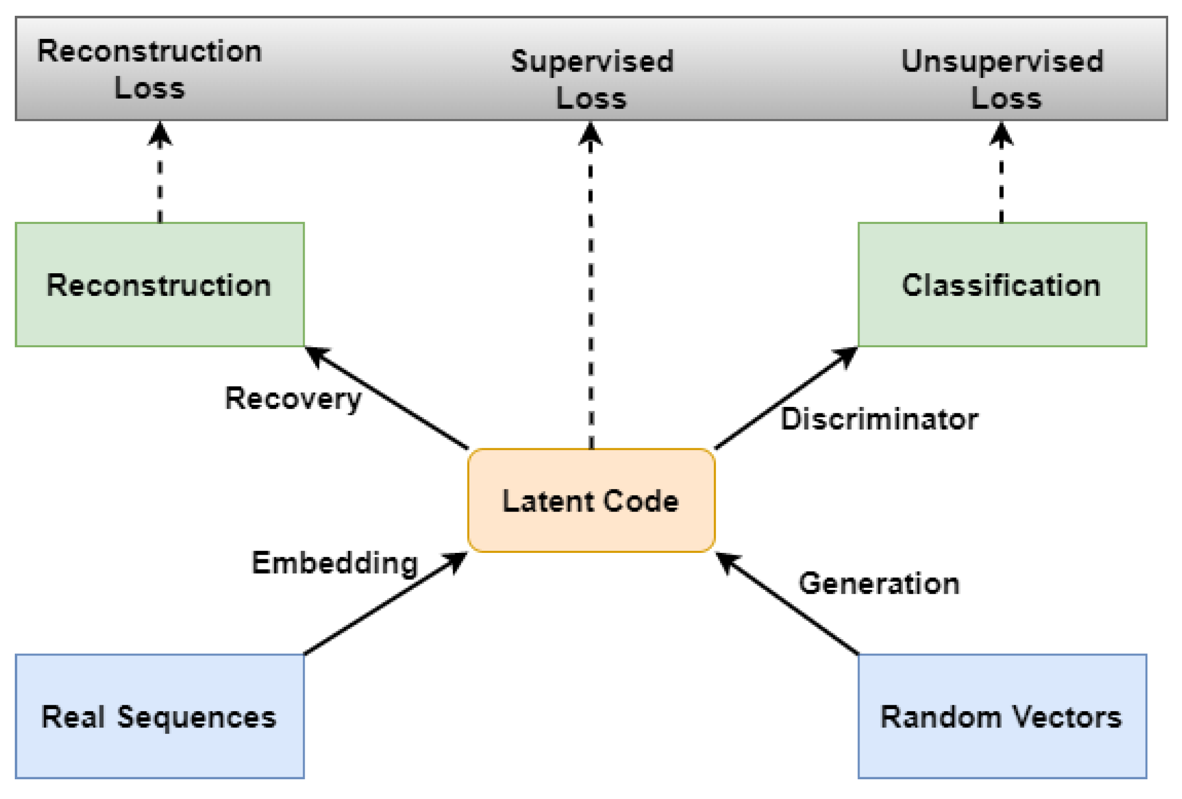
Depending on the number of values recorded, the values in the TS can also be univariate or multivariate. The time-series data typically accept either a real number or an integer value. Jiyoon et al. [8] tested their model on several time-series types and demonstrated that it outperformed previous GAN architectures. The architecture of the TimeGAN as shown in Figure 2 implements the collaborations of a GAN and different components, where G is the generator and D is the discriminator. The GAN is applied with an additional supervised loss on the latent space that was retrieved from the random vectors. They provided a step-wise supervised loss utilizing the original data as supervision in addition to the conventional unsupervised adversarial loss on both real and synthetic data, which aids in learning from the transition dynamics in genuine sequences. Finally, following the training, the false samples are produced using the generator and the classification component. There are three losses [33] defined in TimeGAN [8] that are as follows:

$$L_R=\sum s,x_1:T\sim p\left[\right||s-\widehat{s}{\left|\right|}^2+\sum _t\left|\right|x_t-\widehat{x_t}{\left|\right|}^2]$$

(2)

$$\begin{array}{c}\hfill L_{US}=E_s,x_1:T\sim p[log\left(y_s\right)+\sum _{t}log\left(y_t\right)]+\\ \hfill E_s,x_1:T\sim p\left[\right(log(1-\widehat{y_s})+\sum _t\left(log(1-\widehat{y_t})\right]\end{array}$$

(3)

$$L_S=E_s,x_1:T\sim p[\sum _t\left|\right|h_t-g_x(h_s,h_t-1,z_t){\left|\right|}^2]$$

(4)

where $L_R$ is loss of reconstruction, $L_{US}$ is unsupervised loss, $L_S$ is supervised loss and p is the true distribution. Through back-propagation, the weights of the recovery and embedding functions are updated using the reconstruction loss $L_R$, $\widehat{p}$ is the distribution of the model, x represents the real data, $\widehat{x}$ is the data after reconstruction, and T is the timestamp.

Comparison chart for the related works [8,24,25,26,27,28,29,30] performed in the line of implementing GAN using time-series data is given in

Table 1. Related Works: comparison chart.

S. No.	Paper	Technique Used	Dataset Used	Evaluation Method
1	Mogren et al. [24]	RNN	Classical music dataset	Repetitions and Tone span
2	Ramponi et al. [25]	Time-conditional GAN	Multiple datasets	TSTR
3	Jihoon et al. [8]	TimeGAN	Stock prices and electricity data	Usefulness
4	Hao et al. [26]	Signature Wasserstein-1 (Sig-W1)	Signature dataset	TSTR
5	Sun et al. [27]	DAT-CGAN	Energy and financial dataset	Train Synthetic Test Real (TSTR)
6	Golany et al. [28]	SIMGAN	ECG signals dataset	precision and recall
7	D. Li et al. [29]	MAD-GAN	Water Treatment and distribution datatset	PCA and Discrimination Anomaly Score
8	Wang et al. [30]	SeismoGen	Earthquake dataset	$R^2$

. Table 1 contrasts the related works [8,24,25,26,27,28,29,30] considering the techniques, datasets and evaluation methods used. The reflections of the above papers are discussed in the following Section 3, which explains the challenges faced in dealing with time-series data and the problem statement of the research.

3. Problem Statement

Generative adversarial networks (GANs) [4], which are fundamentally designed to model continuous data but are most frequently used to model images, face a new challenge when modeling continuous time-series data. Time-series problems are made more challenging by the temporal character of continuous data. There are intricate relationships between the temporal features and their characteristics. For instance, when employing multichannel biometric and physiological data, the ECG properties are influenced by the person’s age and health. In contrast to image-based data under a fixed dimension, long-term correlations also exist in the data, which are not always stable in the dimension. Although it is a recognized practice, changing the image size can lower the quality of the image. TimeGAN tried to tackle the temporal dynamics problem of time-series data of GANs.

In TimeGAN, in every stage of training, it is possible to access the distinction between the real and the next-step latent vector (LV), respectively. The unsupervised loss $L_{US}$ trains the generator G to construct real data sequences, while $L_S$, the supervised loss, makes sure that it generates indistinguishable step-wise transitions, but still, it fails to fully capture the features of the multivariate time-series data, and hence, we proposed a novel approach MTS-TGAN to tackle this problem. In the proposed model, we chose to employ a different range of techniques for the model’s evaluation because evaluating GANs for multivariate time-series data is not straightforward and trivial. Hence, we aimed to assert something about the caliber of the generated data. In order to demonstrate that our generated data can be defined from real data samples, we demonstrate the following:

• Behavior of real and synthetic sequences;
• Variety of synthetic sequences;
• Quality of the generated sequences;
• Capturing of the dynamic features of our real dataset by the generator.

A detailed description of the process flow, the proposed model, and its architecture is explained in the next section.

4. Methodology

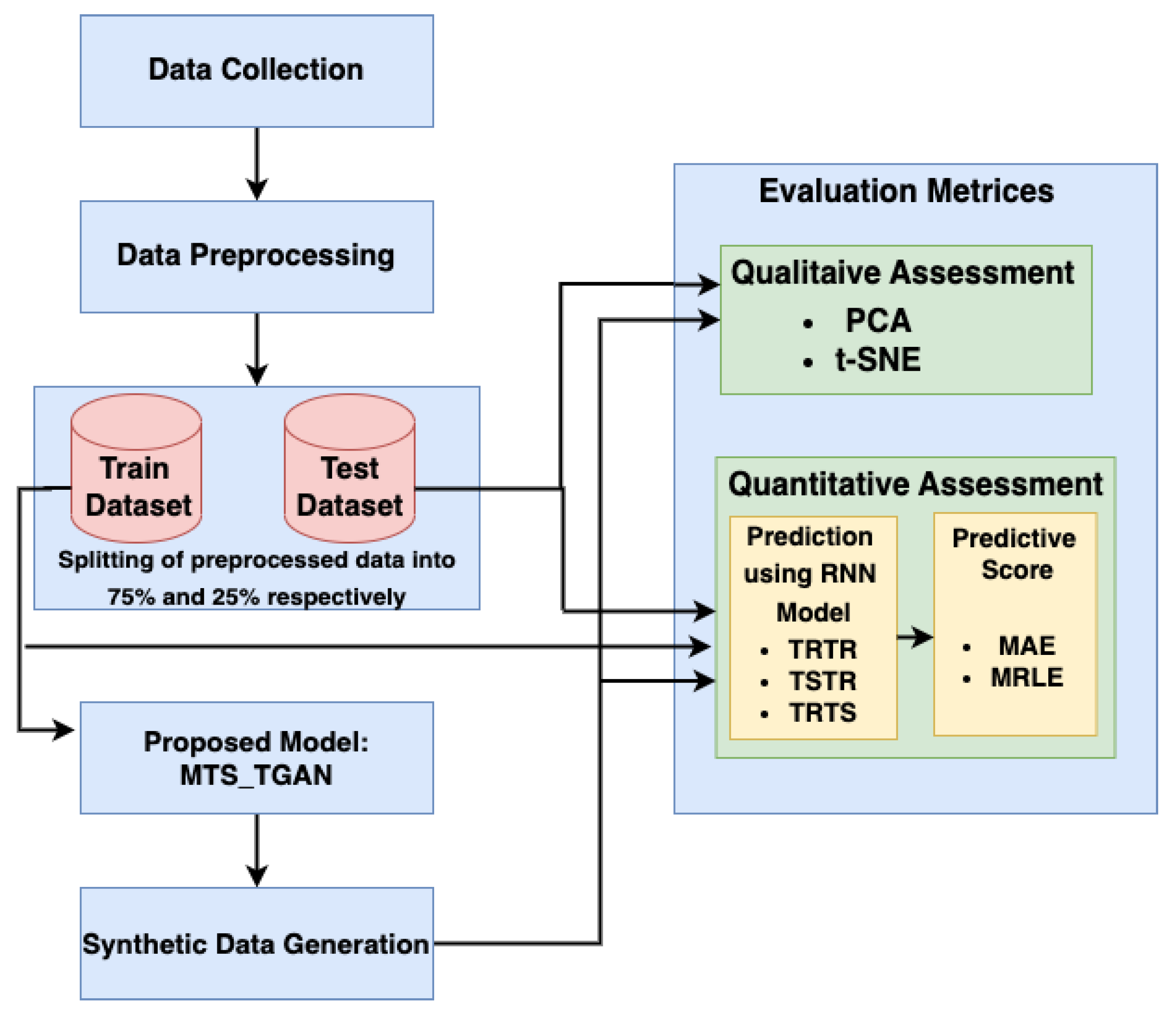
The process flow followed for the design and implementation of the proposed model is shown in Figure 3. The first step is the data collection, then pre-processing of the dataset, followed by a detailed description of the proposed model, and lastly the training and evaluation metrics used for the evaluation of the model as depicted in Figure 3. The elaboration of these steps is given below:

4.1. Data Collection

In this paper, two datasets, namely Google stocks [17] and the UniMIB dataset [18], were used for showing the impact of the proposed model on various parameters. These datasets are briefed below:

• Google Stocks [17]: Data from the Google stock prices dataset, in contrast, are continuous valued but periodic; also, attributes are correlated with one another. We utilized daily data from 2004 to 2021 from Google Stocks, which include aspects such as high, volume, low, adjusted closing, and opening and closing prices. A detailed description of the dataset can be found in [17], and the statistical parameters of the dataset are shown in

  Table 2. Google stocks dataset.

  	Open	High	Low	Close	Adj_Close	Volume
  count	5510	5510	5510	5510	5510	5.51 $\times {10}^3$
  mean	1181.62	1188.49	1173.97	1181.48	1181.48	1.27 $\times {10}^9$
  std	1089.20	1093.80	1083.88	1089.21	1089.21	1.88 $\times {10}^9$
  min	49.27	50.54	47.67	49.68	49.68	7.90 $\times {10}^3$
  25%	268.32	270.77	265.72	268.29	268.29	3.36 $\times {10}^6$
  50%	610.35	616.88	603.04	611.63	611.63	9.58 $\times {10}^6$
  75%	2312.27	2319.23	2295.56	2304.92	2304.92	3.30 $\times {10}^9$
  max	3612.01	3645.99	3600.16	3626.91	3626.91	9.04 $\times {10}^9$

  .
• UniMiB: We chose samples from 24 subjects’ existing recordings and proposed them to 2 groups (Running and Jumping) for the UniMiB dataset [18] in order to train the model.The dataset includes mixed-valued data, which are highly correlated to time stamps and each other; a description of the dataset is shown in

  Table 3. The UniMiB dataset.

  	0	1	2	3	4
  count	30	30	30	30	30
  unique	30	4	15	14	18
  top	1.95, 1.92, …	F	24	168	55
  freq	1	13	6	6	4

  . There are correspondingly 600 samples for each class and 1572 samples. Every sample has 150 timesteps, and each timestep has three accelerator values. Each recording is normalized channel-wise to have a variance of 1 and a mean of 0. A detailed description of the dataset can be found in [18].

4.2. Data Pre-Processing

Prior to synthesizing the data, pre-processing must be ensured due to the varied nature of the data. The six signals’ values in Google stocks [17] fall into varying ranges and exhibit different attributes and characteristics. The Sklearns-Feature selector function [34] is used, which helps in removing the extra noise by outputting important features. Each feature in the dataset is then normalized individually using feature scaling, bringing all values into the range [0, 1], thus normalizing the dataset to ensure that the dataset is consistent. All features have the same format/range. We used the Scikit-MinMaxScaler function [35] and created rolling windows with overlapping sequences of 24 data points [8].

4.3. Proposed Model and Synthetic Data Generation

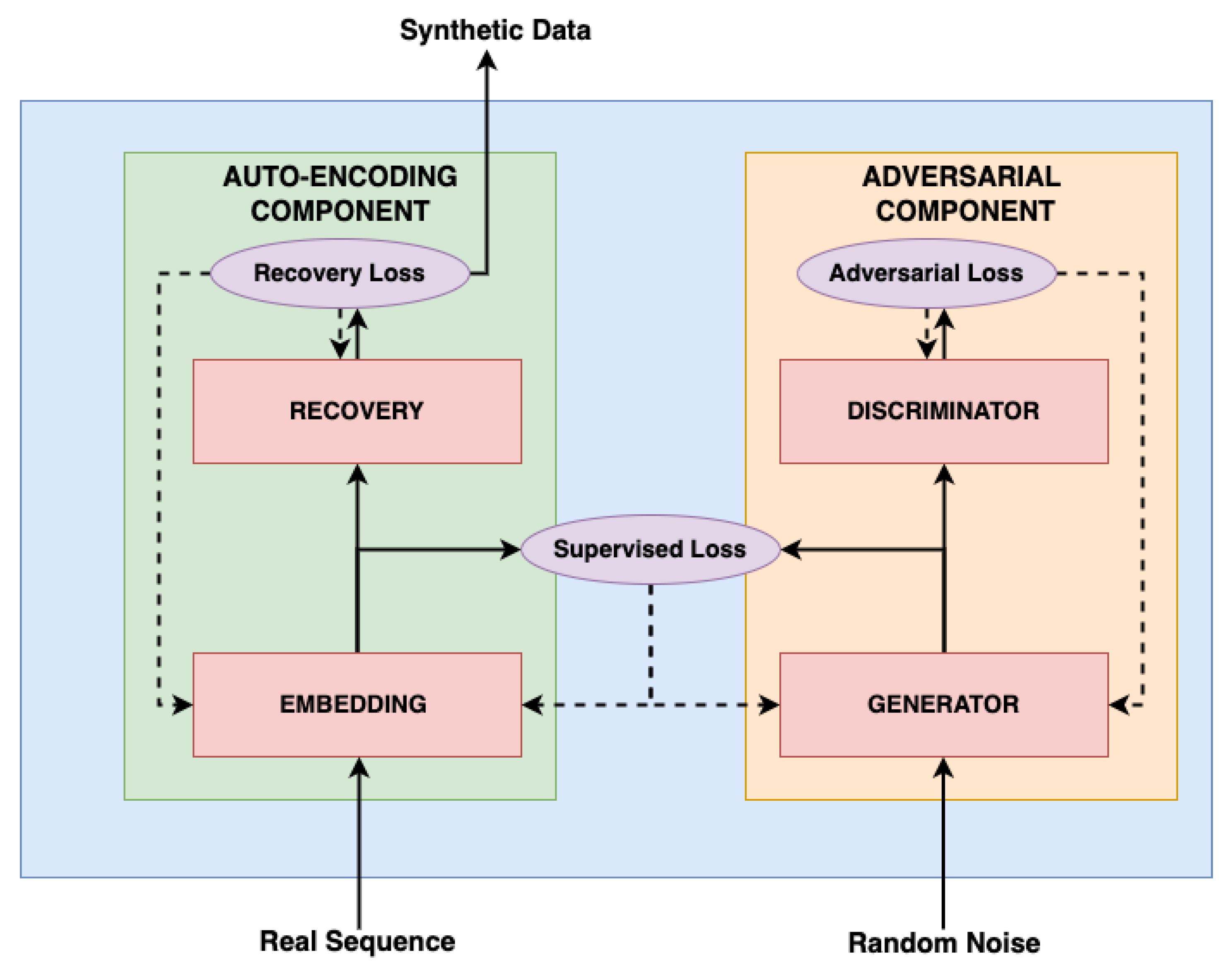
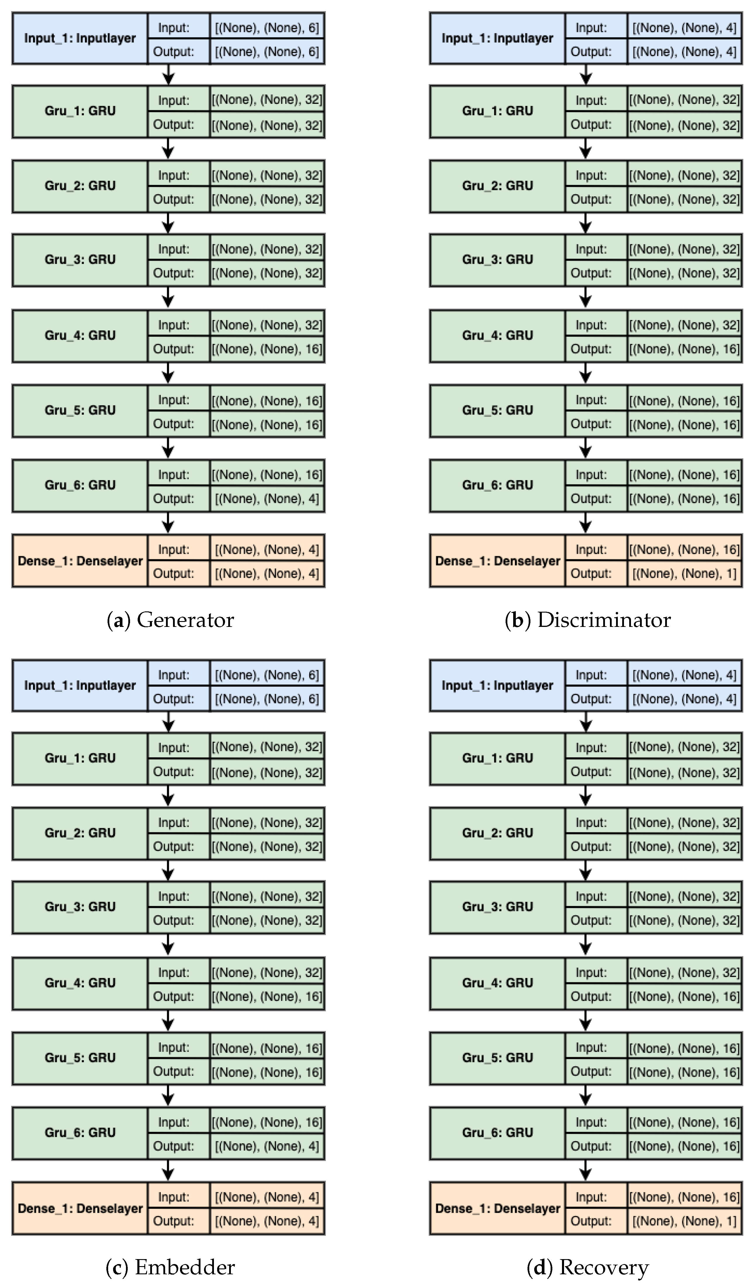
After the pre-processing, the data are then split into 75% and 25% ratios, namely the training and testing datasets, respectively. The training dataset is then fed into the proposed model named MTS-TGAN. MTS-TGAN consists of two components: adversarial and auto-encoder components. The components of MTS-TGAN are shown in Figure 4, wherein the real sequence and random noise act as inputs to the model and at the end, after the overall training and testing, we obtain the synthetic data as an output. Figure 4 clearly shows training and loss functions; components to which loss functions are applied are indicated by dashed arrows, and the data flow is indicated by solid arrows.

The sequence discriminator and generator as well as the recovery and embedding function are the four sub-components that makeup MTS-TGAN. The major finding is that the auto-encoding and adversarial components are trained together so that the proposed model simultaneously learns to encode features, generate sequences and iterate over time. The adversarial network acts in the latent space that the embedding network supplies and a supervised loss synchronize the latent dynamics of both real and synthetic data. Each sub-component is individually described in Figure 5.

The detailed description of the MTS-TGAN architecture is explained further down the section. The overview of the components in the proposed model is shown in Figure 4; all components are composed of an input layer, six GRU layers [15] with 60 s as a sequence length followed by a dense layer [36]. A detailed explanation of each is given as follows:

• Adversarial Component: The generator’s input is a random multivariate noise sequence defined in the feature space of the dataset, which in this case has six dimensions because there are six signals/features present in the data. The latent space, which in this instance was set to four feature spaces, determines the generator’s output. As a result, the generator network’s final layer is dense, consisting of four units. When every neuron in a layer receives input from every neuron in the layer below it, the layer is considered to be dense in a neural network. To make sure that the network terminates in the desired dimension, the dense layer was implemented. Since the discriminator operates in the latent space, its input and output must have the same shape as well as that of the embedder functions. A scalar representing the discriminator’s output indicates whether it believes the sample it was given to be legitimate or bogus. As a result, the discriminator architecture must have a dense layer with one output unit at its end. An overview of these architectures is presented in Figure 5a,b.
• Auto-Encoding Component: The embedding function converts the real data samples into the latent space with 6-dimensional and 4-dimensional latent spaces as input and output, respectively. The embedding function consequently has a dense layer composed of 4 units. The recovery function acts within the latent space, just like the discriminator. Consequently, the embedder’s output shape and input shape are the same as a generator. The recovery function, as opposed to the discriminator, generates reconstructions of the samples back to feature space. As a result, the recovery function has a 6-unit dense layer at its conclusion. An overview of these architectures is presented in Figure 5c,d.

These dimensions are set to “None” to enable the insertion of various values during training and testing that is, simply telling the network that any input parameters are acceptable here when the input is defined by setting these dimensions to “None”. This is essential, as the model should be able to generate samples in multiples and of any sequence length.

The decision to use GRU layers in the proposed model is given to recurrent neural networks (RNNs) [37], which are appropriate for TS data [8,25,26] as analyzed from related works in Section 2. Six stacked GRUs [15], each with 32 units, were used to construct the generator, discriminator, embedder, and recovery function networks in the proposed model. It is possible for a network to learn deeper and more complicated patterns by using stacked GRUs, which is unquestionably the case with six signals, respectively, with various features. Trial and error led to the decision to use six layered GRUs with 32 units on one, two, and three GRU layers followed by 16 units on four, five and six layers.

The generated sequences/samples are then subjected to division into sets for training, testing, and validation. Of the data, 10% is in the test set, 15% is in the validation set, and training is performed with the remaining 75% of the data. Both the generated and the real data samples are subjected to this splitting individually. Now, utilizing datasets based on Train Real Test Synthetic (TRTS), Train Real Test Real (TRTR), and Train Synthetic Test Real (TSTR), the RNN model is implemented for 400 iterations and tested which is explained in the next subsection.

Here, we discuss the training part of the model, but before using the latent codes of the real samples to train the entire model, including adversarial and auto-encoding components together, it was first necessary to pre-train the auto-encoding components to make sure they were relatively representative. One hundred epochs of pre-training were completed, with each epoch denoting a network update following a full run over the training dataset. In the pre and main training, samples from the training dataset were taken from the entire dataset for each epoch.

For convenience and to quickly identify the model with the greatest performance, models were saved for every 1000 epochs during the 50,000 epoch primary training. It was vital to take into account that the best model is not usually the one that has the longest training time. The models would not have been accessible for testing and assessment if they had not been preserved during the training. The generator was trained twice for each epoch to prevent the discriminator from taking over, and a time limit was set for the discriminator’s weight updates. The TimeGAN [8] threshold, which indicated that weights were not changed if the discriminator loss was less than 0.15, was the basis for this.

Table 4. Training parameters of MTS-TGAN.

S. No.	Parameters	Value
1	Sequence Length	60 s
2	No. of samples	32
3	Optimizer	Adam [39]
4	Learning rate	0.0005
5	pre-training epochs No	100
6	No. of epochs	50,000
7	No. of Stacked GRU layers	6
8	No. of units	32 units for layers 1, 2 and 3 and 16 units for layers 4, 5 and 6
9	Loss function LS, LR	MSE
10	Loss function LU	BCE

explains the overall training settings used in the implementation of the model, including parameters from the sequence length to loss function.

Unfortunately, there is no consensus on the metrics for evaluating the generated data for time-series GANs [38] because of the very small number of research that has been published so far. Different strategies have been put forth, but as of now, none has emerged as the leader in the metrics field, and the same applies to the situation of time-series (TS) data. However, we evaluated MTS-TGAN both on qualitative and quantitative metrics, which are described in the next subsection.

4.4. Evaluation Metrics

We evaluated the model on two evaluations: quantitative and qualitative as explained below.

4.4.1. Qualitative Evaluation

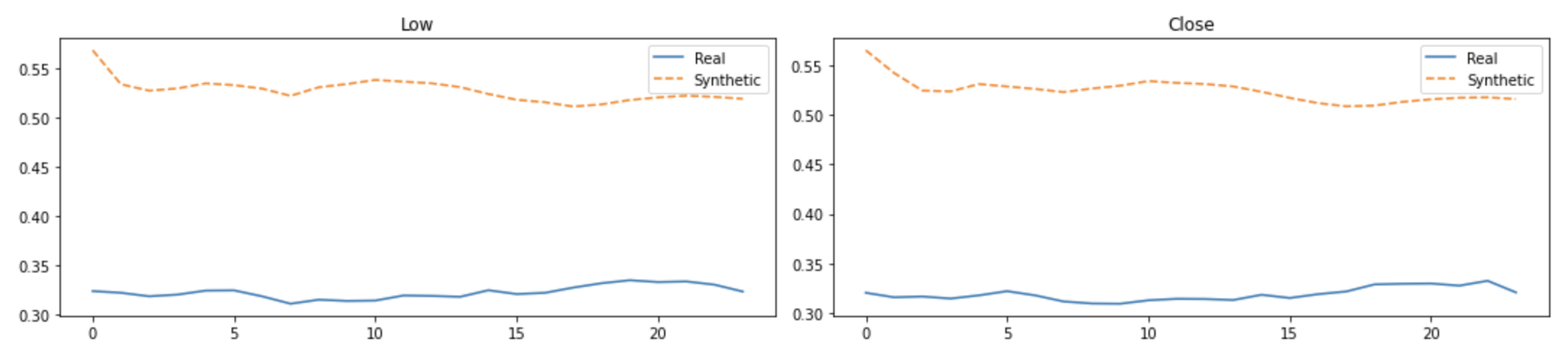
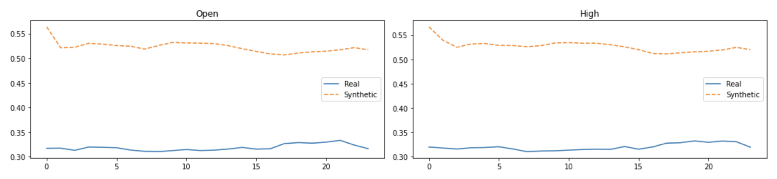
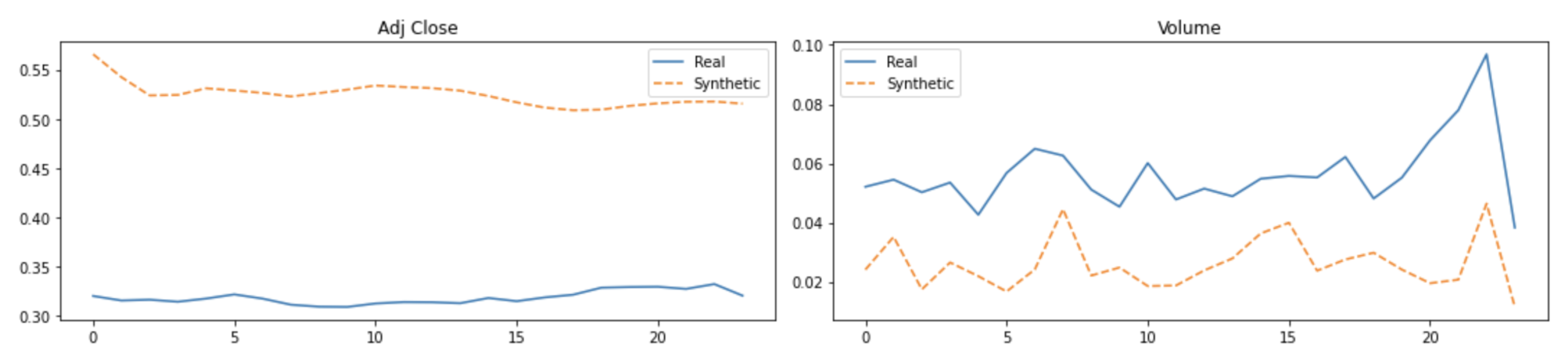
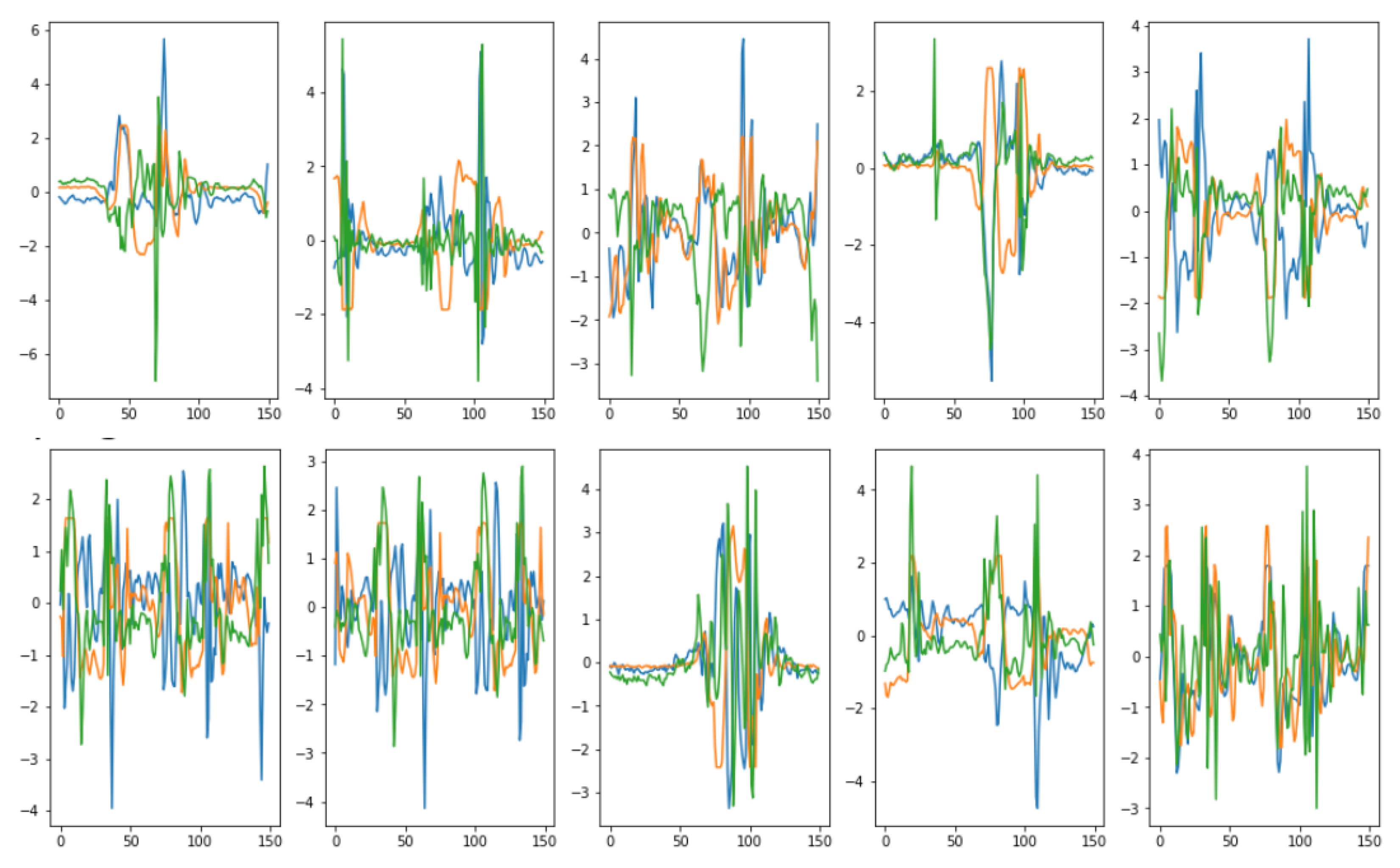
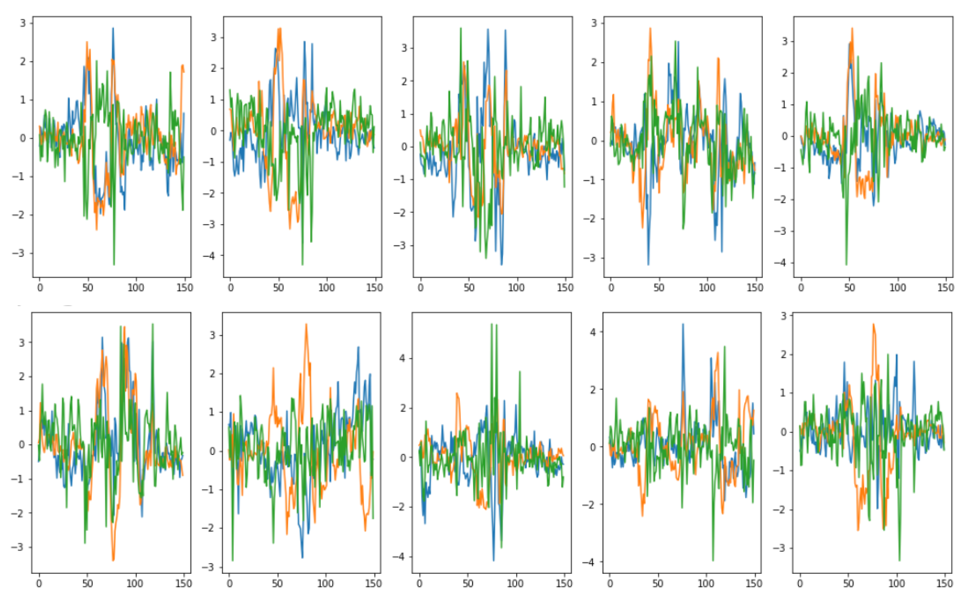
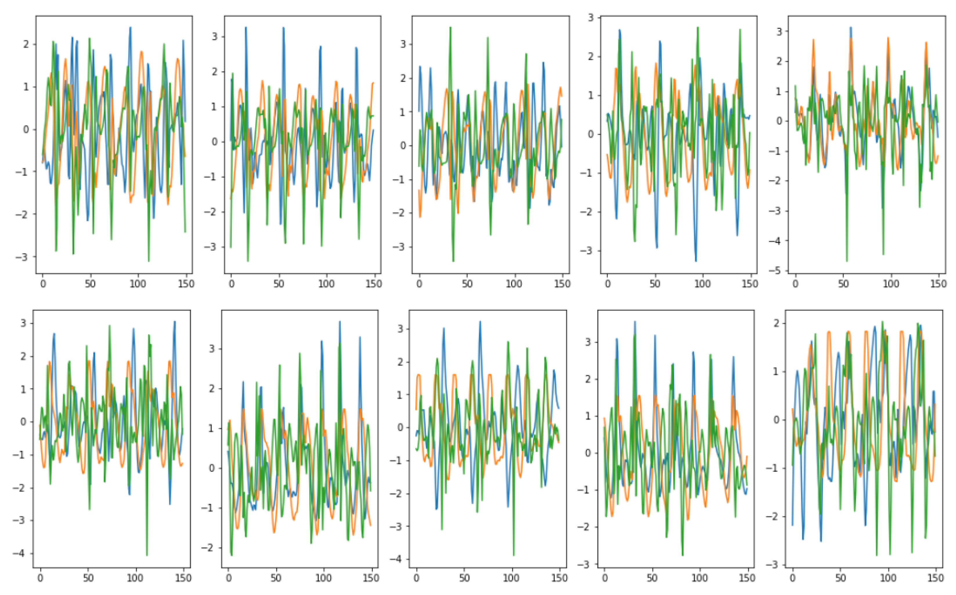
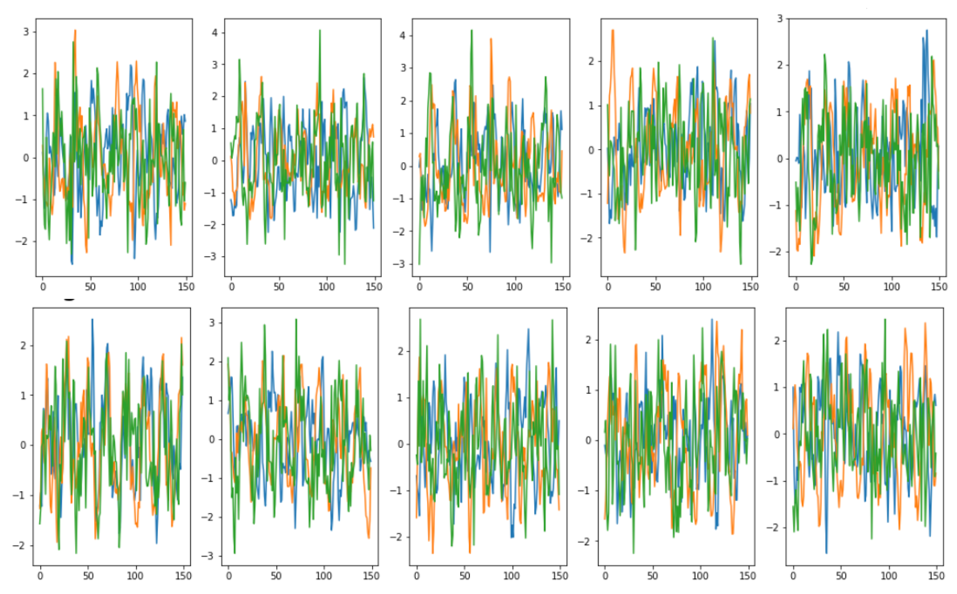
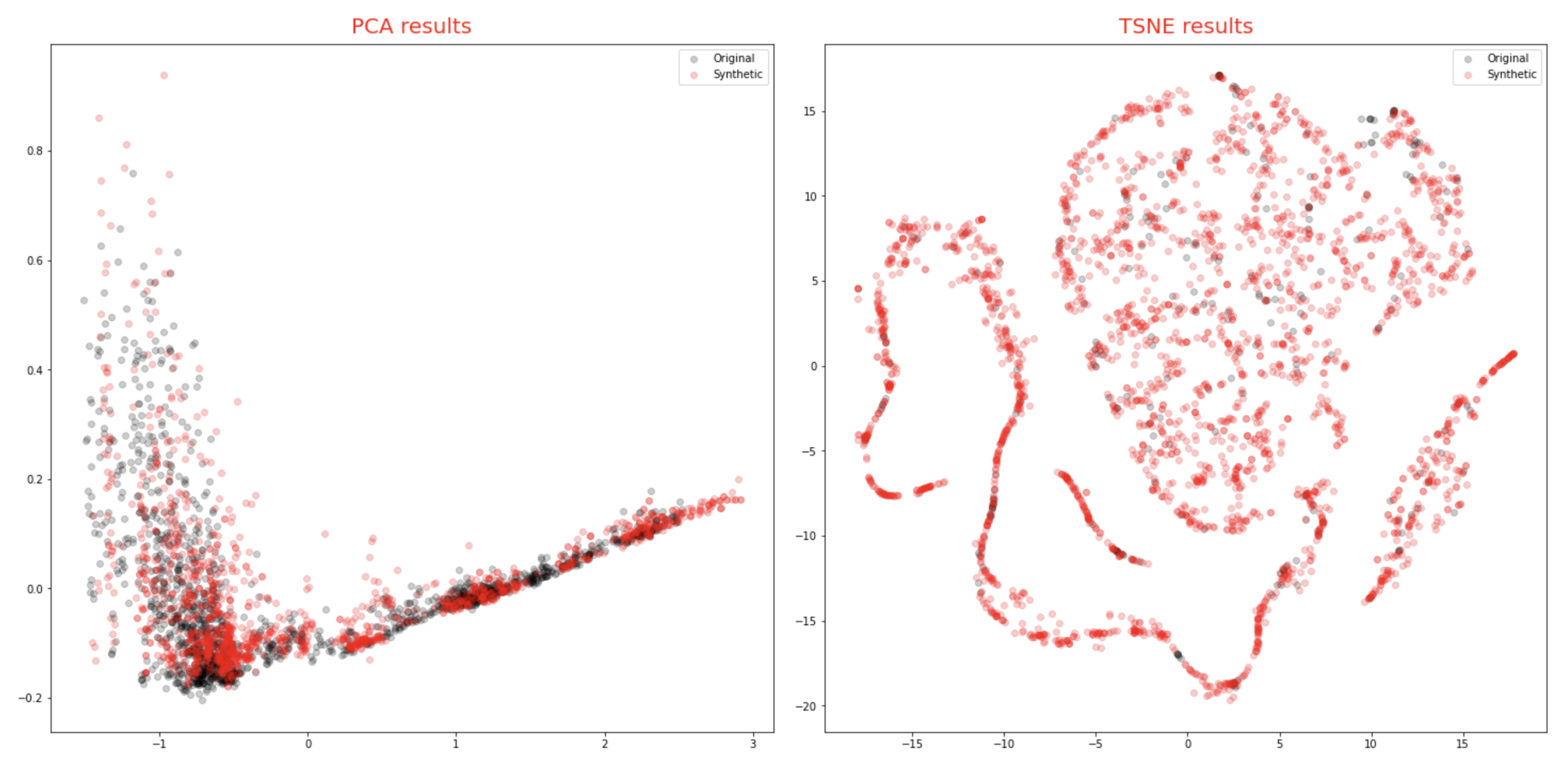
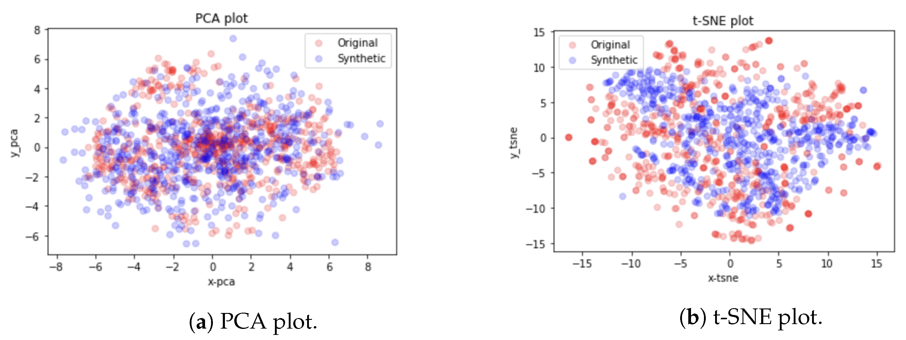
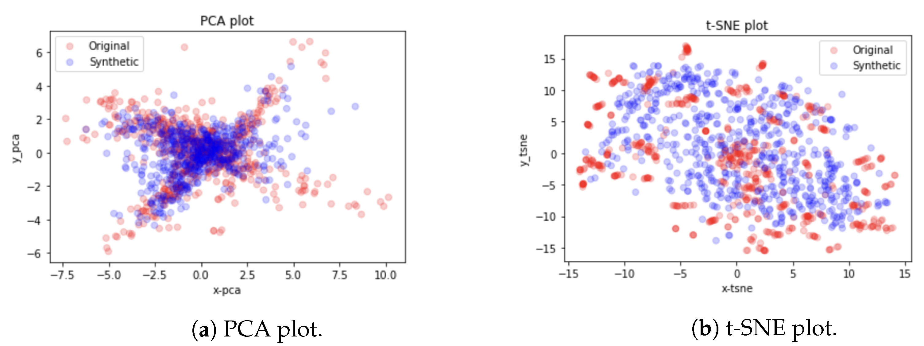
Visual evaluations are typically the focus of qualitative evaluation measures. Different approaches for visualization might be utilized, depending on the task and the model outputs’ format. It is relatively easy to visualize two-dimensional data, but it is more difficult to do so with higher-dimensional (time-series) data. Plotting the created time-series and comparing them to the actual data is the simplest way to visualize the performance of a model.

This might not be sufficient because it is challenging to distinguish tiny differences between actual and synthetic samples. Therefore, it would be impossible to determine whether the model had actually absorbed the entire distribution or not. To address this issue, dimensionality reduction to perhaps two or three dimensions via principal component analysis (PCA) [13] and plotting the findings from that are common approaches to visually evaluating multivariate data [13]. We utilized PCA [13] and t-SNE [14] to convert the multi-dimensional result sequence vectors into two dimensions so that we can visually compare the distribution of the synthetic with actual data values. We also represented the sequences in numeric data form in terms of discriminative and predictive scores as discussed below.

Given that it measures how good the synthetically created data are, the discriminative score can be used to evaluate any GAN model in general. As it demonstrates how well the model caught the temporal dynamics/step-wise dependencies of the data, the prediction score is particular to time-series data. This metric is based on the TSTR training phase, i.e., Train on Synthetic data and Test it on a Real one [7]. On the resulting dataset, we first train a sequence prediction model to determine this measure. We assess this model’s performance using the original data set after training (much as the discriminative score implemented by optimizing a five GRU layer). By figuring out the mean absolute error, we may calculate the predictive score.

4.4.2. Quantitative Evaluation

The regression score is used for comparing a model’s external sources with and without the generated samples. For this, we used a five-layer RNN model. The RNN model comprises of five GRU layers with 32 units and a 6-unit dense layer. Although the RNN model is implemented using the Adam optimizer [39] as well, it uses mean absolute error (MAE), which will be discussed in more detail in the following section, for loss. For training, 6000 samples of 60 s (sequence length) from each data file were selected to construct the data. Then, these samples were divided into sets for training, testing, and validation. Of the data, 10% was in the test set and 15% was in the validation set. Training was done with the remaining 75% of the data. The real data samples and the synthesized samples are treated separately when applying this split. The RNN model is currently trained for 200 iterations and tested using datasets based on TRTS, TRTR, and TSTR.

Two measures are used to assess the RNN model’s performance. The average difference between the true and the anticipated values are measured by the first metric, called mean average error (MAE). Any value between 0 and the MAE score is acceptable; however, the closer the value is to 0, the smaller the difference. In other words, a low MAE score is preferred because it indicates a more accurate prediction. The MAE score is calculated as follows using n as the number of values, $y_i$ as the true value, and $\widehat{y_i}$ as the anticipated value as shown in Equation (5):

$$MAE=\frac{1}{n}\sum _{i-1}^n|y_i-\widehat{y_i}|$$

(5)

The mean squared logarithmic error (MSLE), which can be regarded as a measurement of the percentage difference between the true and projected values, is the second metric. In other words, minor differences between small true and predicted values are managed in a manner that is similar to how large discrepancies between large true and anticipated values are handled. The discrepancy between projected and true values is smaller the lower the MSLE score is, similar to the MAE score. Using the aforementioned definitions, the MSLE score is shown in Equation (6):

$$MSLE=\sqrt{\frac{1}{n}\sum _{i=1}^n(log(y_i+1)-log(\widehat{y_i}+1)){|}^2}$$

(6)

The MTS-TGAN model is assessed using comparisons between the MAE and MSLE on three training phases, namely, TRTR, TSTR, and TRTS methods (explained below).

The RNN model ought to do well in terms of TSTR if it also catches the diversity in the real data. The goal of the evaluation varies depending on which version is used.

• Train Real Test Synthetic (TRTS): It refers to the process of training an external model using real data and then testing it on artificial data (TRTS). By measuring how well the distributions within the genuine data were learned, this method explains how realistic the created data are.
• Train Real Test Real (TRTR): The model is trained and tested on real data (TRTR). This method only serves as a benchmark for Train Real Test Synthetic. Alone, it will not produce any useful results.
• Train Synthetic Test Real (TSTR): The model is tested on actual data after being trained on random data. This method’s goal is to assess how well the differences in the real data are learned as well as how diverse the synthetic data are.

The results of the above methods are shown in Section 5.

5. Results and Analysis

This section deals with the visualization part of the paper and the analysis of the results. The techniques explained in Section 4.3 were implemented on the proposed MTS-TGAN model, and the findings of the same are depicted below.

5.1. Qualitative Scores

After implementing the proposed model, we found that the MTS-TGAN can simultaneously learn to produce representations, encode characteristics and iterate across time. We further compared MTS-TGAN to Time-GAN [8], the best available alternative, and assessed it using qualitative visualizations and quantitative metrics. Graphs of the columns Low, High, Close, Open, Adj Close and Volume of the Google dataset [17] and columns Running and Jumping of the UniMIB dataset [18] are plotted to show the visual representation of the real and the synthetic data. Some generated samples are shown in Figure 6, Figure 7, Figure 8, Figure 9, Figure 10, Figure 11 and Figure 12. Real and synthetic data both continue to be standardized with values between [0, 1] for the Google dataset [17].

Figure 9, Figure 10, Figure 11 and Figure 12 shows the distribution of age, height, and weight of all 30 subjects in the UniMIB dataset [18] as green, orange and blue colors respectively. Figure 9 and Figure 11 show the real data from the UniMIB dataset [18], depicting that the data range from [−3, 3] for the UniMIB dataset, and Figure 6, Figure 7 and Figure 8, Figure 10 and Figure 12 depict the real and synthetic samples of various sequence lengths for the data that are plotted using the Python module, Plotly [40], with the time-steps (seconds) on the x-axis and the signal values on the y-axis. For better visualization, the range of the x-axis is 25 in the case of the Google dataset [17] and 150 for the UniMIB dataset [18].

5.1.1. Raw Visualizations

Instances of synthetic data produced from the real data using MTS-TGAN are displayed in Figure 6, Figure 7 and Figure 8, Figure 10 and Figure 12. We can clearly see from comparing them to the actual data that the synthetic data exhibit visually comparable signal patterns to the actual data.

5.1.2. Visualizations Utilizing PCA and t-SNE

Figure 13, Figure 14 and Figure 15 show visualization example graphs of data point distributions transferred to two dimensions using PCA and t-SNE, which further highlights the resemblance between the real data and synthetic data. These charts show red dots for the original data and blue dots for MTS-TGAN-generated synthetic data. Once more, we see a resemblance in the distribution patterns of the real and synthetic data.

The predictive and discriminator scores show the MAE values in relation to the generated data sequence and the original data sequence, respectively, as shown in

Table 5. Predictive and discriminative scores for Google stocks compared to TimeGAN.

	Predictive Score (Lower the Better)	Discriminative Score (Lower the Better)
TimeGAN [8]	0.037	0.102
Proposed Model	0.024 (13% lower)	0.092 (10% lower)

. However, the predictive and discriminative scores acquired, 0.024 and 0.092, respectively, are still significantly more accurate than the outcomes of the initial implementation [8] by 13% and 10%, respectively, as shown in Table 5.

5.2. Quantitative Scores

The primary concept behind TSTR (Train Synthetic Test Real) is to train the model on synthetic data produced by the model and test it on a held-out set of real data. We chose a straightforward architecture with a five-layer GRU with 20 units to be utilized as a regressor model, which was iterated 400 times.

Table 6. Regression scores.

	MAE	MSLE
TRTR	0.004862	0.000309
TRTS	0.005861	0.000365
TSTR	0.006604	0.000620

displays the regression score of the MTS-TGAN model. The RNN model performs the prediction for both the MAE and MSLE scores more accurately when the scores are close to zero. The TRTS scores are higher than the TRTR values, as expected, indicating that the RNN model performs better on real data than on synthetic data. The scores for TRTR and TRTS in the model are very close to zero, indicating excellent prediction, and the discrepancies between these scores are minimal as shown in Figure 16. The TSTR scores are much higher than the scores of TRTS in terms of both MSLE and MAE for a sequence length of 60 s and iterations.

6. Conclusions and Future Research

The goal of this research was to look at ways to create synthetic time series that are realistic and follow similar distributions of real time-series data. The model and the components were built after performing an extensive literature review. Six stacked GRU layers were used to develop the MTS-TGAN, and the hyper-parameters were selected. The proposed model combines the adaptability of the unsupervised GAN technique with the control over conditional temporal dynamics provided by supervised autoregressive models. MTS-TGAN generates realistic time-series data by utilizing the contributions of the supervised loss and jointly trained embedding network, showing consistent and considerable gains over state-of-the-art benchmarks. This paper concluded that when the MTS-TGAN model was implemented, it produced realistic and varied multivariate time-series data, which were then processed as if they were actual data by external models. The model was evaluated both in terms of qualitative measures, namely t-SNE, PCA, discriminative and predictive scores and quantitative evaluation measures were implemented using an RNN model, which calculated MAE and MSLE scores for three training phases: Train Real Test Real, Train Synthetic Test Real and Train Real and Test Synthetic. The model was able to reduce the overall error up to 13% and 10% in predictive and discriminative scores, respectively.

Despite the encouraging findings of this research, future work may choose to include more features, such as adding more multivariate features or taking a dataset with more multi-modal elements in it so as to assess how well the proposed model handles these additions, or instead of more feature, we can also add different types of data, such as mixed data (which include both tabular data as well as time-series data). It might also be fascinating to combine features with other forms of data, including geospatial data, to create mixed data, as they depend on a number of objects and events. Future research on assessment measures is often required for data production utilizing GANs so that a framework may be agreed upon for a straightforward comparison of findings across investigations.