Active Optics and Aberration Correction Technology for Sparse Aperture Segmented Mirrors

Abstract

Active optics and aberration correction techniques for sparse aperture segmented mirrors are studied. A finite element model of the sparse aperture segmented mirror was established, and a multi-aperture aberration polynomial was derived. According to the hard spot theorem, a co-phase maintenance method based on the change of the edge sensor position in the conventional mode is derived. And a co-phase maintenance method based on the change of the aberration of the segmented mirror surface without the participation of the edge sensor is proposed. The method can correct aberrations of the segmented mirror surface, which are caused by the rigid body displacement along the horizontal direction of the segments. This method can reduce the RMS of the segmented mirror surface to 2.2 nm. The correction principle of the Warping Harness (WH) technique is derived. For the problems of tedious steps and a small number of target aberrations, the correction method is proposed to directly target the aberrations of the segmented mirrors, which is simple and has a wider range of target aberrations. Using this method, the amplitude of each aberration of the stitched mirror is corrected to below ${10}^{-4}\mathrm{nm}$. It is also verified that combining the generalized ridge estimation method and the differential evolution algorithm can effectively solve the correction quantity. Finally, it is verified that the SiC material can effectively improve the adaptability of the segmented mirror to gravity load by reducing the mirror’s weight.

1. Introduction

The completion of Keck I and II telescopes has shown the direction for the further development of large-aperture telescopes. Summarize the current shape of the segment in large segmented telescopes. Furthermore, the hexagonal and circular segments splicing schemes seem more suitable for future large-aperture segmented telescopes [1,2]. Compared with hexagonal segments, circular segments use fewer types of segments for splicing. The processing and preparation process is more mature. The design of the support structure is easier to implement, transplant, and expand. And the R&D is more cost-effective. Meanwhile, Cao Haifeng [3] analyzed that the MTF of different aperture circular and hexagonal segments splicing mirrors are basically the same. This proves the feasibility of using circular segment splicing. In addition, the typical representative of a circular segmented telescope is Giant Magellan Telescope (GMT) [4,5].

The co-phase maintenance technology for the active optics of the segmented telescope is the key to ensuring the imaging quality of the optical system of the segmented telescope. In the traditional model, this technique mainly monitors the relative position of the two segments in real time by the edge sensors, which are located at the edge of the two adjacent spliced segments. Then the correction amount of the displacement actuator is calculated by the active optical control system. Finally, the spliced sub-mirrors are readjusted to the co-phase by adjusting the displacement output of the displacement actuator state [6,7]. Due to the participation of the edge sensor in this mode, the measurement error of the edge sensor will affect the co-phase maintenance accuracy of the mode. Also, the sensor needs to be recalibrated when the temperature and zero drift of the sensor occur. For example, the edge sensor temperature drift of 6 nm/week, 10 nm/week, and 5 nm/month was used by Keck, E-ELT, and TMT telescopes, respectively [8,9,10].

The WH technique can correct the wavefront error of the segmented mirrors with spatial frequencies close to zero. The technique was first applied in the Keck telescope. WH technique is also applied in the two segmented ground-based telescopes, E-ELT, and TMT, which are currently under construction. In the above-mentioned telescope, the correction process of the segmented mirror aberration by this technique is as follows. Firstly, estimate each segment’s surface using the Shack-Hartmann wavefront sensor (SH-WFS) and WH influence function. Secondly, correct the aberration of each segment surface. Then achieve the segmented mirror co-phase by using the traditional co-phase maintenance technique. Finally, reduce the segmented mirror shape introduced due to the sub-mirror surface error [11,12,13,14]. For large-scale segments, stitching of the primary mirror, the process of correcting each segment aberration individually, is very complicated, and the correction time will be very long. While the WH technique only has a certain correction effect on the low-order aberration of the segment surface, which corresponds to a relatively small number of aberrations in the stitching mirror.

This paper presents a combination of theoretical derivation and simulation analysis. Firstly, the polynomial of the aberration of the sparse aperture splicing mirror, the correction principle of the WH technique, and the solution method of the correction amount are derived. Then the co-phase maintenance control model based on the change of the edge sensors indication value in the traditional mode of the sparse aperture splicing mirror is derived. Meanwhile, to address the problem of traditional co-phase maintenance techniques relying on edge sensor measurement accuracy. A co-phase maintenance model based on the segmented mirror aberration evaluation model is proposed, which does not involve edge sensors. The calibration accuracy of two segmented mirror co-phase maintenance models is compared. Finally, we propose a direct correction method of segmented mirror aberration for the complicated correction process of WH technology in the traditional mode.

2. Sparse Aperture Segmented Mirror Aberration Evaluation and Active Optical Control

In this section, we derive the sparse aperture orthogonal polynomial based on the single-aperture Zernike polynomial. The derivation is stemmed from the hard spot localization theory to establish the traditional co-phase maintenance active optical model of the sparse aperture segmented mirror based on the change in the edge sensor position and aberration. Then, In the end, a whiffletree structured triangular plate is taken as an example to derive the correction principle of WH technology.

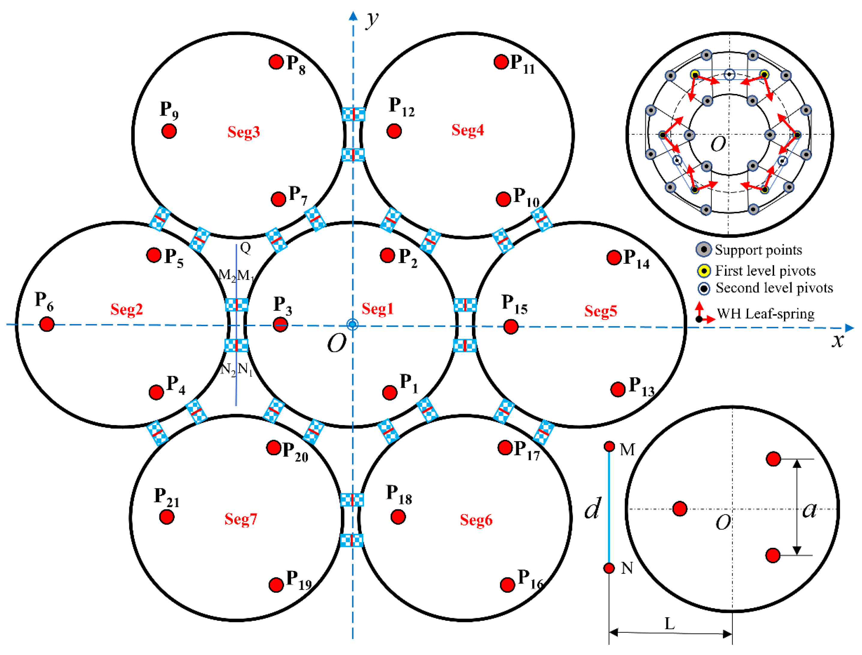
2.1. Segmented Mirror Aberration Mode

A Zernike polynomial defined over a single aperture is a set of continuous complete orthogonal bases, denoted as $Z_i\left(r,\theta \right)$. Suppose there exists a linear irrelevant vector group $B$ in a Euclidean space $V$ such that for all other vectors in the space, it can be represented linearly by $B$. So, the $B$ is the basis of $V$. $Gram-Schimdt$ orthogonalization is the method of transforming a set of irrelevant vector groups in Euclidean space into an orthogonal vector group. The orthogonality of Zernike polynomials in the unit circle region of the sub-aperture is analyzed, and orthogonal normalization is performed to obtain a new set of standard orthogonal polynomials given as follows [15].

$$U_k=\left\{\begin{array}{c}{Z}_1,k=1\\ Z_k-{\displaystyle \sum _{i=1}^{k-1}\frac{(Z_k,U_{i-1})}{(U_{i-1},U_{i-1})}{U}_i (i=2,3,\cdots ,k)}\end{array}\right.$$

(1)

Clearly, $U_k$ can be calculated by iterations. However, this iterative process is computationally difficult and time-consuming. Observing Equation (1), we can see that $U_k$ can be linearly combined with $Z_k$ to form the following relation.

$$U_k={\displaystyle \sum _i^{\mathrm{k}-1}{M}_{ki}{Z}_i}$$

(2)

where $M_{ki}$ is the transformation matrix, and $k$ is the number of polynomials determined for a particular aberration in representing the aberration function. If the set $Z_i$ is known, it is possible to determine the transformation matrix $M_{ki}$, which will make it possible to acquire the orthogonal polynomial $U_k$. The inner product and orthogonality of the polynomials $U_i$ and $U_j$ is defined as follows.

$$〈\left.U_k\right|U_j〉=\frac{1}{A}{\displaystyle {\int }_{{\displaystyle \sum }}{U}_k}{U}_{j}dS={\delta }_{kj}$$

(3)

where $A$ is the area of the integral domain, $dS$ is the integral element on the domain, and ${\delta }_{kj}$ is the Kronecker delta function. Equation (4) is the result of multiplying both sides of Equation (2) with $Z_j$, and Equation (5) is the transpose of Equation (4).

$$〈\left.U_k\right|Z_j〉={\displaystyle \sum _i^{k-1}{M}_{ki}}〈\left.Z_i\right|Z_j〉$$

(4)

$$〈\left.Z_j\right|U_k〉={{\displaystyle \sum _i^{k-1}\left[M_{ki}〈\left.Z_i\right|Z_j〉\right]}}^T={\displaystyle \sum _i^{k-1}\left.〈Z_j\right|Z_i〉}{\left[M_{ki}\right]}^T$$

(5)

Equation (3) can be written as follows.

$$〈\left.U_k\right|U_j〉={\displaystyle \sum _i^{k-1}{M}_{ki}〈\left.Z_i\right|U_j〉}={\delta }_{ij}$$

(6)

Equations (4)–(6) can be written in the following matrix form.

$$\begin{array}{c}{T}_{ZU}=T_{ZZ}{M}^T\\ M{T}_{ZU}=I\end{array}$$

(7)

Solving Equation (7) and substituting $Q={\left(M^T\right)}^{-1}$ yields the following relation.

$$T_{ZZ}=Q^{T}Q$$

(8)

From the Zernike polynomial property of the unit circle, it is known that $T_{ZZ}$ is a symmetric positive definite. Hence, the Cholesky decomposition can be solved to obtain the unique lower triangular matrix $Q$ such that Equation (8) holds, which means $U_k$ can be obtained.

2.2. Segmented Mirror Active Optical Control Mode

2.2.1. Control Model Based on the Variation of the Edge Sensor Position

The principle of co-phase maintenance of Keck telescopes using hexagonal segments for splicing is given in the literature [7], which is mainly based on the hard spot theorem. The traditional co-phase maintenance of the segmented mirror is achieved by exploring the relationship between the position of the hard point and the position of the edge sensor. The axial positioning of the segmented segment in the mirror chamber generally uses three rigid, symmetrically distributed 120° positioning points, called “hard spots.” In the active optical system, the hard spots limit the three degrees of freedom of the segmented segment tip, tilt, and piston.

Considering the segment as a rigid body, as shown in Figure 1, one of the edge sensors on the Seg 1 has coordinates $M_1\left(u,v,0\right)$. The hard spots $P_1(x_1,y_1,0)$, $P_2(x_2,y_2,0)$, and $P_3(x_3,y_3,0)$ on Seg 1 are counterclockwise distributed on the mirror surface in the three-dimensional space. These three points are connected to form an equilateral triangle with the center of gravity at the center of the segment circle and side length $a$. Suppose segment 1 is disturbed by wind load, gravity, temperature, and other external factors. The resulting deviation of the segmented mirror from the coplanar inclination $\theta$ is minimal. Therefore, the changes in the three hard spots in the direction of $X \mathrm{and} Y$ are considered negligible. The coordinates of the $P_1,P_2,P_3$ now become $P_1{}^{\prime }(x_1,y_1,z_1)$, $P_2{}^{\prime }(x_2,y_2,z_2)$ and $P_3{}^{\prime }(x_3,y_3,z_3)$. Similarly, $M_1(u,v,0)$ transforms into $M_1{}^{\prime }\left(u,v,z\right)$. Meanwhile, $M_1{}^{\prime }$ is still in the space plane $O\prime$ formed by the points $P_1{}^{\prime }$, $P_2{}^{\prime }$ and $P_3{}^{\prime }$.

$$z=\left|\begin{array}{ccc}{x}_1-u& y_1-v& z_1\\ x_2-u& y_2-v& z_2\\ x_3-u& y_3-v& z_3\end{array}\right|/\left|\begin{array}{cc}{x}_2-x_1& y_2-y_1\\ x_3-x_1& y_3-y_1\end{array}\right|$$

(9)

From Equation (9), $z$ is a linear combination of $z_1,z_2 \mathrm{and} z_3$ which is given as follows.

$$z=\left(S_1{z}_1-S_2{z}_2+S_3{z}_3\right)/S_0$$

(10)

$S_i(i=0,1,2,3)$ denotes the areas of the triangles $\Delta P_1{}^{\prime }{P}_2{}^{\prime }{P}_3{}^{\prime }$, $\Delta M_1{}^{\prime }{P}_2{}^{\prime }{P}_3{}^{\prime }$, $\Delta M_1{}^{\prime }{P}_1{}^{\prime }{P}_3{}^{\prime }$, and $\Delta M_1{}^{\prime }{P}_1{}^{\prime }{P}_2{}^{\prime }$ respectively, and hold the following relationship.

$$S_0=-S_1+S_2+S_3$$

(11)

As shown in Figure 1, assume that two pairs of adjacent edge sensors are on the intersection of the plane $Q$ and the plane $O^{\prime }$ at a distance of $d$. Let the distance from the center of the circle of Seg 1 to the plane $Q$ is $L$. When the sensors are positioned on the extension of the line connecting the two hard spots, the readings of the edge sensors are insensitive to the displacement of the one remaining hard spot as long as the following condition remains true.

$$\left|\frac{2}{3}(\sqrt{3}L-a)\right|<d<\left|\frac{2}{3}(\sqrt{3}L+a)\right|$$

(12)

The heights of the two edge sensors at $M_1{}^{\prime }$ and $N_1{}^{\prime }$ on Seg 1 are as follows.

$$\begin{array}{c}{z}_{M_1{}^{\prime }}=G_1{z}_1+G_2{z}_2+G_3{z}_3\\ z_{N_1{}^{\prime }}=G_2{z}_1+G_1{z}_2+G_3{z}_3\end{array}$$

(13)

where $G_i=S_i/S_0 \mathrm{with} i=1,2,3$ assuming Equation (12) is satisfied. Similarly, we can obtain the heights of the two edge sensors on Seg 2 after perturbation as follows.

$$\begin{array}{c}{z}_{M_2{}^{\prime }}=R_1{z}_4+R_2{z}_5+R_3{z}_6\\ z_{N_2{}^{\prime }}=R_2{z}_4+R_1{z}_5+R_3{z}_6\end{array}$$

(14)

By defining the sensor reading $H$ as the difference in heights of the sensor positions between two adjacent segments, they can be written as follows.

$$H={\displaystyle \sum _{i=1}^6{C}_i{z}_i}$$

(15)

When the hard spots of two adjacent segments are arranged differently, $C_i(i=1,\cdots ,6)$ is also different. When the segmented mirrors are subjected to wind, gravity, and temperature, the sensor height difference between the segment becomes $H_i,i=1,\cdots ,24$. The corresponding hard spot height becomes $z_i,i=1,\cdots ,21$, which gives the following relation.

$$A_{24\times 21}\cdot z_{21\times 1}=H_{24\times 1}$$

(16)

where $A$ is the stiffness matrix between the hard spot $Z$ directional displacement and the variation in the position of the edge sensor. Let the solved residuals of $H$ are represented as $v_H$, then it can be written in the following fashion.

$$v_H=A\hat{z}-H$$

(17)

where $\hat{z}$ is the estimated value of $z$. $\hat{H}=A\hat{z}$ is the estimated value of $H$. the evaluation function of the correction quantity is represented as $MSE(\hat{H})$.

2.2.2. Control Model Based on Aberration Evaluation Model

The current co-phase maintenance technology is mainly implemented by edge sensors and displacement actuators, which are overly dependent on the measurement accuracy of the edge sensor. In addition, when the segment diameter thickness is relatively large, and the number of support points is small, the mirror body at the edge sensor installation position undergoes large deformation. At the same time, due to the edge sensor temperature, zero drift and other errors exist, which will lead to aberration correction transfer efficiency being reduced. This reduces the segmented mirror co-phase maintenance accuracy.

It is assumed that under ideal co-phase detection conditions, the mirror aberration $U_k$ can be used as an evaluation criterion, mainly when active optics are utilized to adjust the segmented mirror from out of phase to a co-phase state. Suppose a hard spot $P_i$ in the segmented mirror goes up along $Z-axis$, then the specular aberration changes to $\Delta U_{ki}$. According to Section 2.2.1, when the segmented mirror is subject to gravity and temperature until the hard spot position in the segment becomes $z_i^{\prime },i=1,\cdots ,21$, the aberration of the out-of-phase segmented mirror is $U_k^{\prime }$ The change of height $\Delta z$ can be expressed in terms of out-of-phase aberration of the segmented mirror $U_k^{\prime }$ as follows.

$$\Delta z\cdot \Delta U_k=U_k^{\prime }$$

(18)

In Equation (18), $\Delta U_k$ is the stiffness matrix between the hard spot displacement and the aberration variation.

$$\Delta U_k=\left[\Delta U_{k1},\Delta U_{k2},\cdots ,\Delta U_{k21}\right]$$

(19)

Let the solved residuals of $U_k$ are represented as $\Delta$, and it is given in the following equation.

$$\Delta =\Delta \hat{z}\cdot \Delta U_k-U_k^{\prime }$$

(20)

where $\Delta \hat{z}$ is the estimated value of $\Delta z$. Suppose ${\hat{U}}_k^{\prime }=\Delta \hat{z}\Delta U_k$ is the estimated value of $U_k^{\prime }$, then the evaluation function of the correction quantity is $MSE({\hat{U}}_k^{\prime })$.

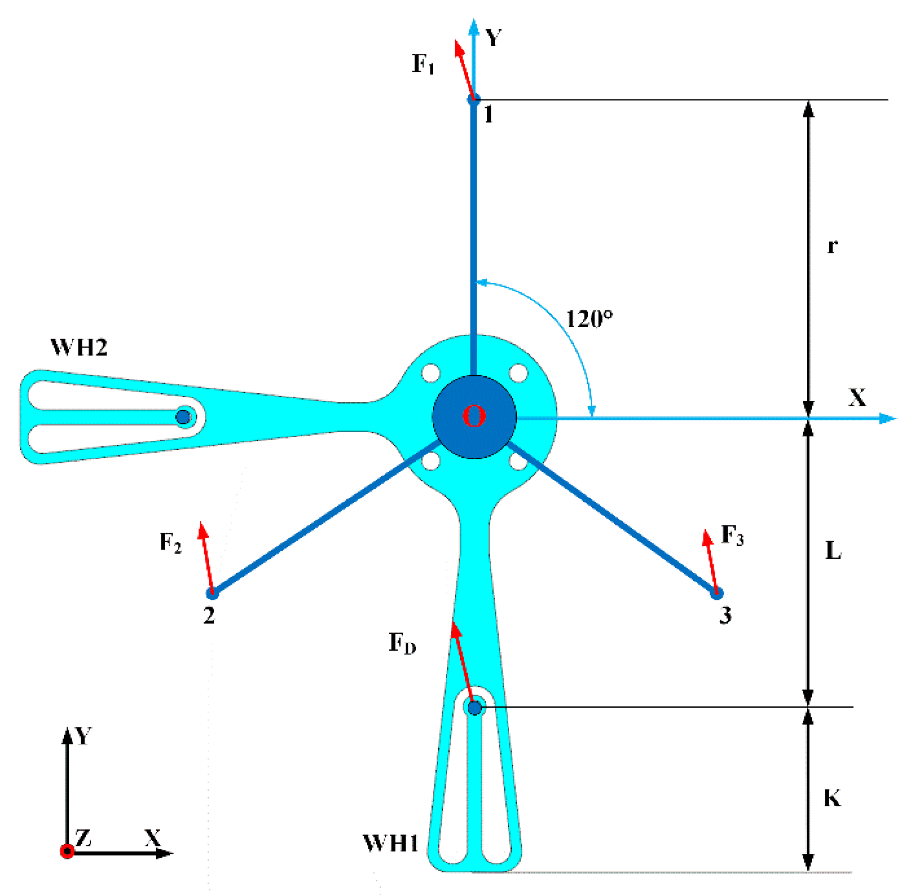
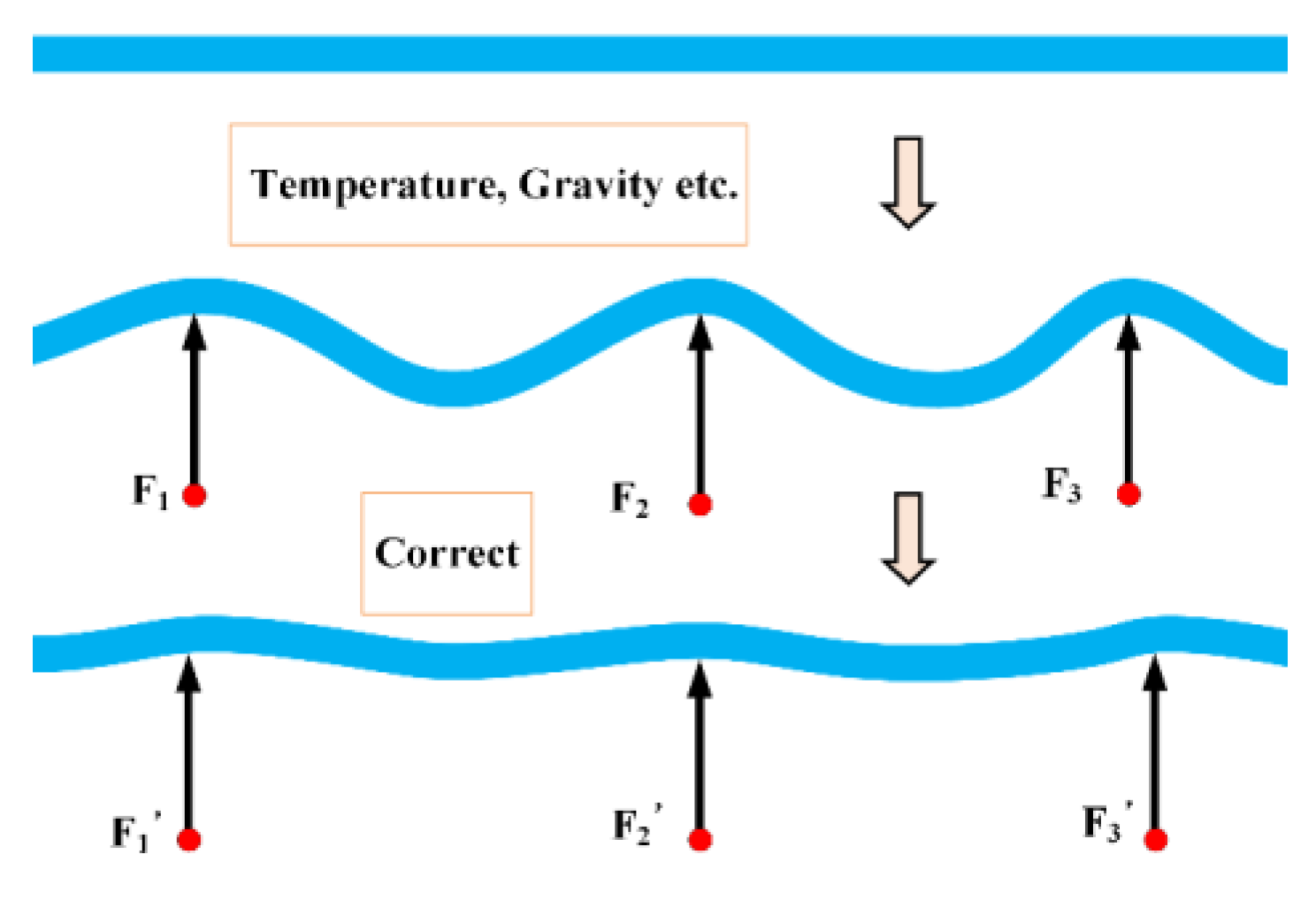
2.3. Warping Harness Technique Calibration Principle

WH technology corrects the surface shape error of the mirror with the help of its elastic deformation. This correction method is based on the law of linearity and convergence. The WH spring plate is directly connected to the triangle plate in the Whiffletree structure. The actuator pushes the end of the spring plate to convert the correction force into a correction torque applied to the triangular plate. Thus, changing the magnitude of the force on the three axial flexible rods connected to the triangular plate can correct the surface shape. The purpose of the correction is to change the force on the three axial flexible rods connected to the triangular plate. Let us take an equilateral Whiffletree triangle as an example, shown in Figure 2. When $F_D=0$, the following relation can be established.

$$F_1=F_2=F_3=G/3$$

(21)

In Equation (21), $F_1, F_2 \mathrm{and} F_3$ are the reaction forces along the Z-direction at the three points of the triangle. When a force $F_D$ is applied along the Z-direction at WH1, a moment of the $F_D(L+K)$ is generated on the triangle. At this point, $F_1, F_2 \mathrm{and} F_3$ transform into $F_1^{\prime }, F_2^{\prime } \mathrm{and} F_3^{\prime }$.

$$\left\{\begin{array}{l}{F}_1^{\prime }=F_1+\Delta F_1\\ F_2^{\prime }=F_2+\Delta F_2\\ F_3^{\prime }=F_3+\Delta F_3\\ F_1^{\prime }+F_2^{\prime }+F_3^{\prime }=G\\ \Delta F_{1}r-\Delta F_{2}r/2-\Delta F_{3}r/2=F_D(L+K)\end{array}\right.$$

(22)

According to the symmetry and deformation coordination conditions, the following equality holds.

$$\Delta F_2=\Delta F_3$$

(23)

Moreover, $\Delta F_1$ can be expressed as follows.

$$\Delta F_1=2\Delta F_2=F_D(L+K)/2r$$

(24)

A schematic diagram of the mirror distortion during correction is shown in Figure 3.

From Equation (24), the force applied to the spring plate can cause a change in the supporting force of the Whiffletree self-balancing structure. Assuming that when one of the force actuators outputs $F_D=1N$, the axial support rod is subjected to a change in force $\Delta F$ resulting in the deformation $W_i(x,y)$ of the segmented mirror surface. When the actuator outputs a force $F_{Di}, i=1,2,\cdots ,n$, where $n$ is the total number of WH actuators in the segmented mirror support system, the total deformation of the mirror surface can be expressed in the following equation.

$$W(x,y)={\displaystyle \sum _{i=1}^n{F}_{Di}}{W}_i(x,y)$$

(25)

Suppose the current specular error is $W_D$ and $E$ is the stiffness matrix of the WH relative to the specular aberration. To produce a deformation of $W_D$ requires the actuator to apply a correction force of magnitude $f$.

$$Ef=W_D$$

(26)

When $W_D$ is expressed using the segmented mirror aberration $U_D$ introduced in Section 2.1, Equation (26) takes the following form.

$$Ef=U_D$$

(27)

The following equation is obtained after solving for the residuals $v_U$.

$$v_U=E\hat{f}-U_D$$

(28)

where $\hat{f}$ is the estimated value of $f$ when the estimated value of $U_D$ is ${\hat{U}}_D$. Then the evaluation function of the correction quantity is $MSE({\hat{U}}_D)$.

3. Correction Quantity-Solving Method

In this section, an improved generalized ridge estimation is proposed to solve for the correction quantities. These quantities are required in the mirror correction by the segmented mirror co-phase maintenance and WH techniques. These correction quantities are also needed to solve for the ridge and weight matrix in the iterative process using an improved differential evolution algorithm.

3.1. Improved Generalized Ridge Estimation

Let the measurement parity model is given below.

$$\left\{\begin{array}{c}{L}_L=A_L{X}_L+{\Delta }_L\\ E({\Delta }_L)=0,\mathrm{cov}({\Delta }_L)={\sigma }_0^{2}I\end{array}\right.$$

(29)

where $L_L$ is the observation vector of order $n\times 1$; $A_L={(a_1,a_2,\cdots ,a_n)}^T$ is the design matrix of order $n\times t$; $X_L$ is the parameter vector of order $t\times 1$, ${\Delta }_L$ is the observation error vector of order $n\times 1$, and ${\sigma }_0$ is the unit weight error. The corresponding error equation is given in the following equation.

$$v=A_L{\hat{X}}_L-L_L$$

(30)

where $v$ is the residual vector, and ${\hat{X}}_L$ is the estimated value of $X_L$. The ordinary least squares estimation of $X_L$—which is referred to as the $LS$ estimate—is given in Equation (31).

$${\hat{X}}_{LLS}={(A_L^T{A}_L)}^{-1}{A}_L^T{L}_L$$

(31)

The corresponding influence function is defined in the following fashion.

$$IF(L_{Li};{\hat{X}}_L)=-{(A_L^T{A}_L)}^{-1}{a}_i^T{v}_i$$

(32)

It can be seen that the influence function depends on three factors: the normal matrix $A_L^T{A}_L$, the row vector $a_i$, and the residual vector $v$. When the design matrix $A_L$ contains complex covariance, which means the normal matrix $A_L^T{A}_L$ is sick, some of its eigenvalues ${\lambda }_j$ are close to 0. Although ${\hat{X}}_{LLS}$ has the smallest variance in the linear unbiased estimation, its mean square error $MSE({\hat{X}}_{LLS})={\sigma }_0^2{\displaystyle \sum _{i=1}^t\frac{1}{{\lambda }_i}}$ becomes large as a result.

The solution accuracy of $z$, $\Delta z$ and $f$ in Equations (16), (18) and (27) may be degraded due to the sickness of the normal matrices $A^{T}A$, $\Delta U_k{}^T\Delta U_k$ and $E_U{}^T{E}_U$ significantly when solving them using the ordinary least squares after segmented mirrors under load.

It is crucial to address the effect of $a_i$ in Equation (29) by considering them far away from each of the other points $a_j$. First, an appropriate weight is added to $a_i$. It is done by giving a smaller weight $p_i$ to $a_i$ when it is far away from the other $a_j$. It is called $GM$ estimation [16]. An improved generalized ridge estimation, also called $GL$ estimation, is proposed to overcome the effect of normal matrix pathology on the estimation while resisting the effects of observation coarseness and high leverage points. It is done by combining $LS$ estimation and $GM$ estimation, establishing the following solution equation.

$${\hat{X}}_{GL}={\left(A_L^T{P}_L{A}_L+\eta I\right)}^{-1}{A}_L^T{P}_L{L}_L$$

(33)

In the above equation, $P_L=diag(p_1,p_2,\cdots ,p_n)$ is the weight matrix and $\eta$ is the ridge parameter. Equation (33) is generally solved iteratively. If the parameter valuation at step $l$ has been solved with a solution ${\hat{X}}_{GL}^{(l)}$, observed residual $v_i^{(l)}=A_L{\hat{X}}_{GL}^{(l)}-v_i^{(l-1)}$, and a ridge parameter ${\eta }^{(l)}$, then the solution at step $l+1$ is as follows.

$${\hat{X}}_{GL}^{(l+1)}={\left(A_L^T{P}_L^{(l+1)}{A}_L+{\eta }^{(l+1)}I\right)}^{-1}{A}_L^T{P}_L^{(l+1)}{v}_i^{(l)}$$

(34)

When the number of iterations is $n$, the total observed residuals are calculated as $v_{GL}=A_L{\hat{X}}_{GL}^{}-L_L$, where ${\hat{X}}_{GL}={\displaystyle \sum _{l=1}^n{\hat{X}}_{GL}^{(l)}}$, such that the estimated value of $L_L$ is ${\hat{L}}_L=A_L{\hat{X}}_{GL}$. Afterward, the accuracy evaluation function is solved as $MSE({\hat{L}}_L)$, similar to $MSE(\hat{H})$ introduced in Section 2.2.1, $MSE({\hat{U}}_k^{\prime })$ presented in Section 2.2.2, and $MSE({\hat{U}}_D)$ discussed in Section 2.3.

3.2. Improved Differential Evolution Algorithm

Equation (34) requires recalculation of the weight matrix $P_L$ and the ridge parameter $\eta$ in each iteration step, which is done by the differential evolution algorithm, also known as the DE algorithm in this work.

The basic idea of the DE algorithm is to use 2 randomly selected different vectors in the population to interfere with the existing vectors. Each vector in the population is disturbed, and the new vectors replace the previous generation if the corresponding fitness function is smaller than their previous generation [17,18]. The DE algorithm reduces the probability of falling into a local solution by using real-number encoding. It is to find the optimal solution efficiently. The implementation DE algorithm is expressed in Equations (35)–(39). Each individual in the population represents a set of solutions in the solution space. A single individual can be expressed as follows.

$$X_{i,G}=(x_{1,i,G},x_{2,i,G},...,x_{M,i,G})$$

(35)

where $i$ represents the $i^{th}$ individual in the solution space. $M=n+1$ represents the dimension of the solution vector, such that $x_{1,i,G}=\eta$, and $x_{j,i,G}=p_{j-1},j=2,3,\cdots ,M$. $G$ represents the current evolutionary generation. To ensure that the initial population is spread throughout the solution space, the slant tent chaotic mapping function is chosen to initialize the population. The implementation can be seen in the following equation.

$$\begin{array}{c}{x}_{j,1,0}=rand(0,1)\times (x_{j,\max }-x_{j,\min })+x_{j,\min }\\ X_{j,i,0}=\left\{\begin{array}{ll}\frac{x_{j,(i-1),0}}{rand(0,1)},{\mathrm{x}}_{\mathrm{j},(\mathrm{i}-1),0}\in [0,\mathrm{rand}(0,1))\hspace{0.33em}& \\ \frac{1-x_{j,(i-1),0}}{(1-rand(0,1))},{\mathrm{x}}_{\mathrm{j},(\mathrm{i}-1),0}\in [\mathrm{rand}(0,1),1]\hspace{0.33em}& \end{array}\right.\end{array}$$

(36)

where $x_{j,max} \mathrm{and} x_{j,min}$ represents the upper and lower bounds of the optimization parameters given by $j$. Traversing the entire solution space of the function avoids getting into local solutions and speeds up the convergence of the algorithm. The premature problem is avoided, and the performance of the algorithm is improved by the variational mixture approach of Equation (37).

$$V_{i,G}=X_{i,G}+0.5\times F_s\times (R_B\times (X_{best,G}-R_B\times X_{i,G}))$$

(37)

In the above equation, $R_B$ is a random constant obeying normal distribution and $X_{best,G}$ represents the best individual in the G^th generation. The population size $NP\ge 4$. $F_s$ is the scaling factor and takes values in the range $[0.0001,1]$. In each generation, two individuals are generated by both mutations, and the one with high fitness is selected as the next generation individual. This improvement of multiple variants competing with each other allows the DE algorithm to have a fast convergence speed and increase the population diversity, improving searchability. The crossover operation can be expressed as follows.

$$u_{j,i,G}=\left\{\begin{array}{ll}{v}_{j,i,G}\hfill & ,\mathrm{rand}(0,1)\le \mathrm{CR}\hfill \\ x_{j,i,G}\hfill & ,other\hfill \end{array}\right.$$

(38)

where $v_{j,i,G}$ represents the $j^{th}$ element of the vector $V_{i,G}$ and $CR$ is the crossover probability. The selection operation can be expressed in the following fashion.

$$X_{i,G+1}=\left\{\begin{array}{ll}{U}_{i,G}\hfill & ,\mathrm{f}(X_{i,G})\le \mathrm{f}(U_{i,G})\hfill \\ X_{i,G}\hfill & ,other\hfill \end{array}\right.$$

(39)

In the above equation, $U_{i,G}$ is a vector composed of $u_{j,i,G}$ and $f$ is the fitness function. From the implementation of the DE algorithm, we can find that the more critical operational steps are for the variation and crossover operations, among which the selection of the scaling factor $F_s$ and the crossover probability $CR$ is crucial. When the crossover probability $CR$ of the system is designed to be larger, the population changes faster. Moreover, the damage to the best-adapted individuals is also larger. On the contrary, the population evolves slowly, and the search speed decreases [19]. Thus, the crossover probability $CR$ can reflect the global search ability and local search ability of the algorithm. The designs of $F_s$ and $CR$ in the DE algorithm were set as an adaptive function of the fitness function. The idea of dominant poles is adopted in selecting the fitness function. Firstly, the system indicators are calculated as a second-order system with 2 poles ${\lambda }_{1,2}$ as the dominant poles of the system. The definition of the fitness function is given in Equation (40).

$$\begin{array}{l}{E}_E=1+G({\lambda }_{1,2})\\ J={\mathrm{Re}}^2\left\{E_E\right\}+{\mathrm{Im}}^2\left\{E_E\right\}\end{array}$$

(40)

where $E_E=0$ is the characteristic equation of the system. $\mathrm{Re}$ and $\mathrm{Im}$ are the real and imaginary parts, respectively. At this time, the DE algorithm selects the individual with a small adaptation as the next generation in the selection operation by trying to make $E_E({\lambda }_{1,2})=0$. The evaluation function of the DE algorithm is set for the accuracy of parameter solving in the GL estimation process, as shown in the following equation.

$$E_{DE}=\frac{1}{1+MSE({\hat{X}}_{GL})}$$

(41)

If the solution of Equation (41) is close to 1, the solution is more accurate.

4. Simulation Verification

In this section, the finite element method is used to build a sparse aperture segmented mirror system consisting of seven sub-apertures to verify the algorithms proposed in Section 2 and Section 3. It is also to compare the co-phase maintenance accuracy of two active optical control modes of segmented mirrors and to verify the correction capability of the WH technique for wavefront aberration of segmented mirrors.

4.1. Segmented Mirror System Development

A thin mirror with a diameter of $\varphi 500\mathrm{mm}$, a radius of curvature of 6 m, an edge thickness of 25 mm, and a material of Zerodur was used as the segments. A segment support system was developed using an optimized design with 18-point Whiffletree supports in the segment axial direction, 12 correction forces per support system to achieve WH technical correction, and 3-point tangential rod-type supports in the lateral direction. According to Figure 1, the splicing distance is 5 mm.

The room temperature was set to 20 °C along with three load conditions. T condition had a temperature increase of 10 °C. The Y and Z conditions were gravity loads along the segmented mirror optical axis pointing horizontally and zenith. Analyses were done for these three conditions, and the mirror surface shape error was calculated. The residual deformation of the segmented mirror surface is shown in Figure 4. The data units in the figure are in nm.

It can be seen that the segmented mirror deformation is larger under the gravity load, and the mirror deformation generated by the temperature is small. Therefore, the active optical control model is used for the Y and Z conditions to achieve co-phase maintenance. The WH technique is used for the T condition to correct the segmented mirror aberration.

4.2. Segmented Mirror Active Optical Control

Two schemes were used to correct the segmented mirror error introduced by gravity load discussed in Section 4.1. Scheme 1 is the active optical control model based on the change in the edge sensor position, and this scheme was derived in Section 2.2.1. Scheme 2 is the active optical control model based on the aberration evaluation model proposed in Section 2.2.2.

For Scheme 1: First, the stiffness matrix $A_{12\times 21}$ is established by applying unit forced displacement to each hard spot position of the segmented mirror system, respectively. Then the edge sensor position-variation matrix $H_Y^{(0)},H_Z^{(0)}$ is established under Y and Z working conditions. The correction process is as follows. Firstly, according to Equation (16) and the algorithm in Section 3, the vector dimension $M=21+1=22$ is solved. With the number of individuals in the population as 220, the evolutionary algebra $G=50$, the crossover probability $CR=0.8$, and the amount of change in height for each hard spot $z_Y^{(0)},z_Y^{(0)}$ is solved and substituted into the model. The remaining amount of change in the position of the edge sensor after corrections $H_Y^{(1)}, \mathrm{and} H_Z^{(1)}$ is calculated. It is a cyclic process of active optical correction of the segmented mirror and generally takes 2–3 cycles to entirely correct $H_Y^{(0)}$ and $H_Z^{(0)}$.

For Scheme 2: Similar to Scheme 1, the unit forced displacement is applied to each hard spot, respectively, and the mirror deformation is decomposed according to Equation (1). Then, the stiffness matrix $\Delta U_k$ is established. Afterward, the mirror aberration matrix is obtained for Y and Z conditions $U_{kY}^{\prime (0)} \mathrm{and} U_{kZ}^{\prime (0)}$. The correction process is the same as that of Scheme 1. According to Equation (18) and the algorithm in Section 3, the change in the height of each hard spot $\Delta z_Y^{(0)},\Delta z_Z^{(0)}$ is calculated and substituted into the model. The residual of the mirror aberration after corrections $U_{kY}^{\prime (1)} \mathrm{and} U_{kZ}^{\prime (1)}$ is calculated. The loop is run $t$ times until $U_{kY}^{\prime (t)}-U_{kY}^{\prime (t-1)} \mathrm{and} U_{kZ}^{\prime (t)}-U_{kZ}^{\prime (t-1)}$ are less than the finite element solution accuracy.

The residual deformation of the segmented mirrors after correction by the two schemes is shown in Figure 5.

In Scheme 1, the edge sensor value indicates the Z-directional rigid body displacement of the mirror surface. Because there is a certain angle between each segment surface upon splicing, different rigid body displacements along X and Y directions are observed between Seg 1 and the remaining 6 segments. It makes the residual error of the segmented mirror surface larger when the displacement of the edge sensor is corrected to 0. It also reflects that during the design of the segment support system, the rigid body displacement of the segment’s surface along X and Y directions should be strictly set according to the requirements of co-phase accuracy of the segmented mirror surface at the same time, which means that the design and processing requirements of the support system are improved to a certain extent, and the processing and manufacturing costs are increased.

In Scheme 2, because the correction object is the wavefront aberration of the segmented mirror, it can be regarded as the aberration of the local position of the segmented mirror in the X and Y directions of each segment. The correction object is also reflected in the numerical magnitude of the aberration. Therefore, the correction accuracy of this scheme is higher, and the residual error of the mirror after correction is small. At the same time, Scheme 2 can reduce the complexity of the control system because there is no edge sensor involved. Thus improving the control efficiency and enhancing the segmented mirror co-phase maintenance cost performance.

In summary, the co-phase maintenance model proposed in Section 2.2.2 reduces the control system complexity and support system design and processing requirements and improves the co-phase maintenance efficiency and cost-effectiveness compared to the traditional model without the involvement of edge sensors.

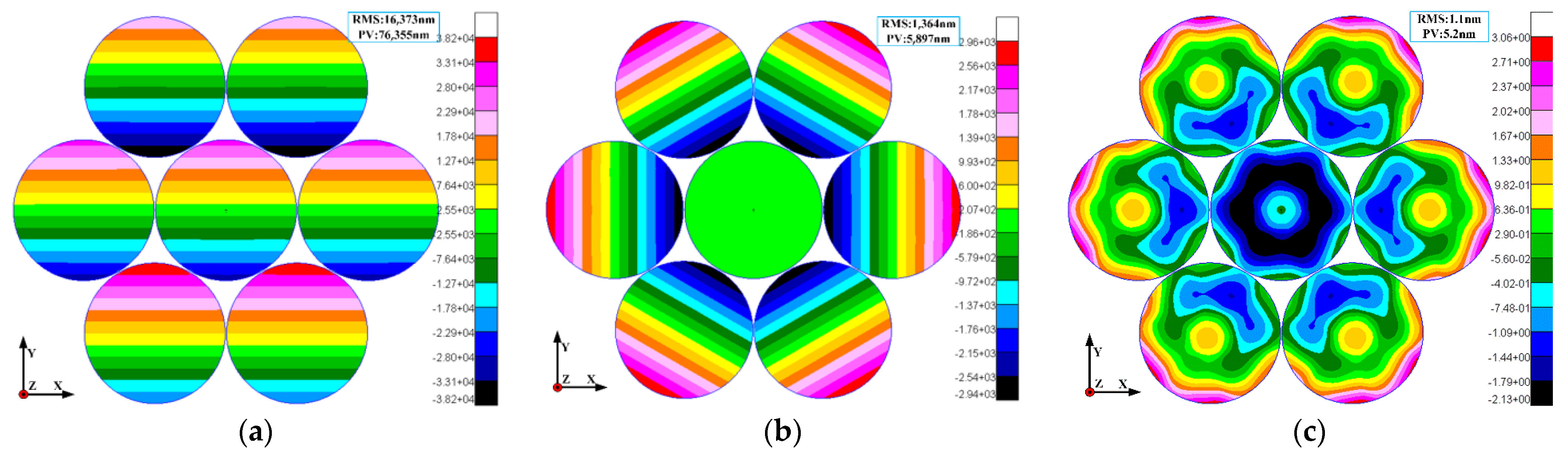
4.3. Segmented Mirror Aberration Correction

In Section 4.2, the co-phase maintenance accuracy of the two segmented mirror control modes was verified and compared. In this section, the WH technique is presented to correct the residual error of the mirror after the segmented mirror is in the co-phase state as per Scheme 1 presented in Section 4.2. WH technique is also used to correct the mirror error under the T condition. As in Section 4.2, Scheme 1 is set as an aberration correction mode with the segmented mirror aberration as the correction target. While Scheme 2 is the correction of the segment’s aberration followed by the co-phase maintenance of the segmented mirror by using the conventional co-phase retention technique as mentioned in the literature [11,12,13,14].

In Scheme 1, the WH stiffness matrix $E$ is obtained by applying a unit force to the end of the WH spring leaf in the segment system and fitting it according to Equation (1). For the residual aberrations of the segmented mirror surface after the correction done by Scheme 1 presented in Section 4.2, $Y \mathrm{and} Z$ conditions are set as $U_{DY}^{(0)}$ and $U_{DZ}^{(0)}$. Moreover, the aberrations of the segmented mirror surface in $T$ condition are set as $U_{DT}^{(0)}$. Similar to the correction process discussed in Section 4.2, the aberrations of the segmented mirror surface after the first correction are calculated according to Equation (27) and the algorithm in Section 3. It is done with the solution vector dimension $M=12\times 7+1=85$, the number of differential evolutionary populations of 850, the evolutionary algebra $G=50$, the crossover probability $CR=0.8$, and the actuator correction forces $f_Y{}^{(0)},f_Z{}^{(0)} \mathrm{and} f_T{}^{(0)}$. Finally, these values are substituted into the model. The residuals of $U_{DY}^{(1)}$, $U_{DZ}^{(1)}$ and $U_{DT}^{(1)}$ are calculated. It is assumed that the change in the correction forces $\Delta f=f^{\left(t\right)}-f^{\left(t-1\right)}$ is smaller than $\xi ={10}^{-6}\mathrm{N}$ after $t$ cycles, and the correction is cut off.

In Scheme 2, firstly, the correction force and segment surface aberration stiffness matrix of the segment system are established. Then, each segment surface shape error is analyzed under Y, Z and T working conditions. The sub-aperture aberration coefficient matrix is fitted according to the Fringe Zernike polynomial $Z_{Yi}^{(0)},Z_{Zi}^{(0)},Z_{Ti}^{(0)}$. Where Y, Z and T in the subscript represent the Y, Z and T conditions. $i$ represents the segment code as shown in Figure 1. According to Equation (27) and the algorithm in Section 3, this is done with the solution vector dimension $M=13$, the number of differential evolutionary populations of 130, the evolutionary algebra $G=50$, and the crossover probability $CR=0.8$, when $\Delta f=f^{\left(t\right)}-f^{\left(t-1\right)}$ is smaller than the accuracy of the finite element software solution $\xi ={10}^{-6}\mathrm{N}$, the segment aberration correction is finished. Then the segmented mirror co-phase maintenance is carried out according to Scheme 1 in Section 4.2. The comparison of residual deformation of Scheme 1 and Scheme 2 in this section is shown in the following figure.

It can be seen that the two schemes adopted in this section are from Figure 6, which have improved the face shape accuracy to different degrees after mirror correction. Among these, the correction effect of Scheme 1 is the most obvious, with the RMS value decreasing from 149.3 nm to 2.2 nm in the Z condition. This indicates that Scheme 1 can effectively correct the segmented mirror error introduced by the rigid body displacement along the X and Y directions of the segment and the residual aberration of the segment together.

It can be seen from Figure 7 that Scheme 1 can correct the magnitude of each order of aberration of the segmented mirrors below ${10}^{-4}\mathrm{nm}$. Figure 7a shows that Scheme 1 has an obvious correction effect on the aberration of the segmented mirrors. The implementation of Scheme 2 only corrects the aberrations of the segment. So Scheme 2 in this section only has a certain correction effect on certain aberrations.

In summary, by comparing the two segmented mirror correction methods through the finite element method, we can obtain the aberration correction mode proposed in this paper with the segmented mirror aberration as the correction target, which has a simple correction method, a wider target aberration range and higher accuracy.

4.4. SiC Material Segmented Mirror Active Optical Control

Based on the segmented mirror support system developed in Section 4.1, the segment material is replaced with SiC. Adjust the segment material to SiC, and adjust the segment thickness according to the principle of equal stiffness until the mirror surface shape accuracy is equal for Zerodur and the SiC segment in Y and Z conditions.

This section is about the sparse aperture segmented mirror error of the SiC segment introduced by Y and Z working conditions. Schemes 1 and 2, similar to Section 4.2, are utilized to implement the co-phase correction for the segmented mirrors under the Y and Z conditions. The correction steps are the same. The residual deformation of the segmented mirrors after the co-phase correction of the two schemes is shown in Figure 8.

Comparing Scheme 1 and Scheme 2 in Figure 8, we can get that because of the smaller thickness and lighter mass of the SiC segment, the rigid body displacement along the X and Y directions under gravity load is smaller. It reflects the advantage of SiC material in the thin mirror technology and the adaptability of the support structure. Comparing the results of the analysis of the Zerodur material segmented mirrors in Section 4.2, it can be found that the residual deformation of the SiC material segmented mirrors is smaller after correction, thus confirming the excellent adaptability of the SiC material segmented mirrors to gravity loads.

5. Conclusions

In the paper, the active optics and aberration correction technology for sparse aperture segmented mirrors are investigated and analyzed using a GMT-type segmented mirror model as an example. The sparse aperture orthogonal polynomial is derived using Gram-Schimdt orthogonalization based on the single-aperture Zernike polynomial. From the hard spot theorem, the active optical model of the sparse aperture segmented mirror based on the variation of the edge sensor position is established. The active optical control of the segmented mirror is proposed with the segmented mirror aberration as the evaluation function. The correction principle of the WH technique is derived by taking a Whiffletree triangular plate as an example. By improving the existing ridge estimation and the differential evolution algorithm, the ridge parameters and the weight matrix in the iterative process of the correction volume are solved by combining the two methods.

Through theoretical analysis and simulation verification, the following conclusions can be drawn.

(1)

The active optical control model based on aberration evaluation mode and the active optical control model based on the change of edge sensor position can realize the active optical correction of segmented mirrors. However, the aberration evaluation mode has a relatively high correction accuracy. It does not depend on the edge sensor, which reduces the complexity of the co-phase maintenance method and improves the cost performance of the technique;

(2)

Compared with the traditional segmented mirror aberration correction method, the proposed aberration correction mode with the segmented mirror aberration as the correction target, which has a simple correction method, a wider target aberration range and a better correction effect;

(3)

The combination of the improved generalized ridge estimation proposed in this study and the improved differential evolution algorithm can be used to efficiently and accurately solve the correction quantity. Introducing the ridge parameter and the weight matrix results in a full-rank normal matrix and dramatically improves the degree of the sickness of the control matrix;

(4)

SiC material is superior to Zerodur material for thin mirror technology and support system adaptability. Using SiC as a segmented mirror material can effectively reduce the quality of the support system while improving the face shape accuracy of the segmented mirror after co-phase.

It is shown that the active optical control model based on the aberration evaluation model of the segmented mirror can be used to maintain the co-phase. The WH technique is used to correct the residual aberration of the segmented mirror after co-phase. The combination of generalized ridge estimation and differential evolution algorithm is used to solve the correction quantity, which can effectively reduce the number of normal matrix conditions and achieve an accurate Solving accuracy. Using SiC material for the segmented segment can effectively reduce the support system mass and improve the adaptability of the gravity load on the segmented mirror surface. This study provides a new solution to the problem of co-phase maintenance q e and aberration correction of the segmented mirror surface and the choice of mirror material.

References

1. Nelson, J.E.; Mast, T.S. Construction of the keck observatory. In Advanced Technology Optical Telescopes IV; SPIE: Washington, DC, USA, 1990; pp. 47–55. [Google Scholar]
2. Medwadowski, S.J. Structure of the Keck telescope—An overview. Astrophys. Space Sci. 1989, 160, 33–43. [Google Scholar] [CrossRef]
3. Cao, H.F. Research on the Technologies of Active Optics for Large-Aperture Segmented Optical/Infrared Telescope. Ph.D. Thesis, University of Chinese Academy of Sciences (Changchun Institute of Optics, Fine Mechanics and Physics, Chinese Academy of Sciences), Changchun, China, 2020. [Google Scholar]
4. Johns, M.; McCarthy, P.; Raybould, K.; Bouchez, A.; Farahani, A.; Filgueira, J.; Jacoby, G.; Shectman, S.; Sheehan, M. Giant magellan telescope: Overview. Ground-Based Airborne Telesc. IV 2012, 8444, 526–541. [Google Scholar]
5. GMT Organisation. GMT System Level Preliminary Design Review–Telescope (Section 6); GMT Organisation: Atlanta, GA, USA, 2013. [Google Scholar]
6. Bouchez, A.H.; Angeli, G.Z.; Ashby, D.S.; Bernier, R.; Conan, R.; McLeod, B.A.; Quirós-Pacheco, F.; van Dam, M.A. An overview and status of GMT active and adaptive optics. Adapt. Opt. Syst. VI 2018, 10703, 284–299. [Google Scholar]
7. Jared, R.C.; Arthur, A.A.; Andreae, S.; Biocca, A.K.; Cohen, R.W.; Fuertes, J.M.; Franck, J.; Gabor, G.; Llacer, J.; Mast, T.S.; et al. WM Keck Telescope segmented primary mirror active control system. In Advanced Technology Optical Telescopes IV; SPIE: Washington, DC, USA, 1990; Volume 1236, pp. 996–1008. [Google Scholar]
8. Minor, R.H.; Arthur, A.A.; Gabor, G.; Jackson Jr, H.G.; Jared, R.C.; Mast, T.S.; Schaefer, B.A. Displacement sensors for the primary mirror of the WM Keck telescope. In Advanced Technology Optical Telescopes IV; SPIE: Washington, DC, USA, 1990; Volume 1236, pp. 1009–1017. [Google Scholar]
9. Mast, T.; Chanan, G.; Nelson, J.; Minor, R.; Jared, R. Edge sensor design for the TMT. In Ground-Based and Airborne Telescopes; SPIE: Washington, DC, USA, 2006; Volume 6267, pp. 974–988. [Google Scholar]
10. Wasmeier, M.; Hackl, J.; Leveque, S. Inductive sensors based on embedded coil technology for nanometric inter-segment position sensing of the E-ELT. In Ground-Based and Airborne Telescopes V; SPIE: Washington, DC, USA, 2014; Volume 9145, pp. 647–659. [Google Scholar]
11. Han, L.; Liu, C.; Fan, C.; Li, Z.; Zhang, J.; Yin, X. Low-order aberration correction of the TMT tertiary mirror prototype based on a warping harness. Appl. Opt. 2018, 57, 1662–1670. [Google Scholar] [CrossRef] [PubMed]
12. Weisberg, C.L.; Colavita, M.; Cole, G.; Nissly, C.R.; Rogers, J.; Schöck, M.; Seo, B.-J.; Troy, M. Experimental data improves prediction of Thirty Meter Telescope segment warping harness correction. In Modeling, Systems Engineering, and Project Management for Astronomy IX; SPIE: Washington, DC, USA, 2020; Volume 11450, pp. 248–261. [Google Scholar]
13. Mast, T.S.; Nelson, J.E. Fabrication of large optical surfaces using a combination of polishing and mirror bending. In Advanced Technology Optical Telescopes IV; SPIE: Washington, DC, USA, 1990; Volume 1236, pp. 670–681. [Google Scholar]
14. Nijenhuis, J.; Hamelinck, R.; Braam, B. The opto-mechanical performance prediction of thin mirror segments for E-ELT. In Modern Technologies in Space-and Ground-Based Telescopes and Instrumentation II; SPIE: Washington, DC, USA, 2012; Volume 8450, pp. 90–98. [Google Scholar]
15. Dai, G.M.; Mahajan, V.N. Nonrecursive determination of orthonormal polynomials with matrix formulation. Opt Lett. 2007, 32, 74–76. [Google Scholar] [CrossRef] [PubMed]
16. Rousseeuw, P.J.; Hampel, F.R.; Ronchetti, E.M.; Stahel, W.A. Robust Statistics: The Approach Based on Influence Functions; John Wiley & Sons: Hoboken, NJ, USA, 2011. [Google Scholar]
17. Noman, N.; Iba, H. Accelerating Differential Evolution Using an Adaptive Local Search. IEEE Trans. Evol. Comput. 2008, 12, 107–125. [Google Scholar] [CrossRef]
18. Richard, G.L. Designing Nonstandard Filters with Differential Evolution. In Streamlining Digital Signal Processing: A Tricks of the Trade Guidebook; IEEE: Piscataway, NJ, USA, 2007; pp. 25–32. [Google Scholar]
19. Yu, W.; Liang, H.; Chen, R.; Wen, C.; Luo, Y. Fractional-order system identification based on an improved differential evolution algorithm. Asian J. Control. 2022, 24, 2617–2631. [Google Scholar] [CrossRef]
Figure 1. Schematic diagram of the segment arrangement.
Applsci 13 04063 g001
Figure 2. Schematic diagram of WH calibration.
Applsci 13 04063 g002
Figure 3. Schematic diagram of the calibration process.
Applsci 13 04063 g003
Figure 4. Mirror deformation under load, (a) Deformation of mirror surface in Y condition, (b) Deformation of mirror surface in Z condition, (c) Deformation of mirror surface in T condition.
Applsci 13 04063 g004
Figure 5. Zerodur segment segmented mirror surface after correction by two schemes, (a) Scheme 1, deformation of mirror surface in Y condition, (b) Scheme 1, deformation of mirror surface in Z condition, (c) Scheme 2, deformation of mirror surface in Y condition, (d) Scheme 2, deformation of mirror surface in Z condition.
Applsci 13 04063 g005aApplsci 13 04063 g005b
Figure 6. Residual deformation of the mirror surface after aberration correction for Scheme 1 (top) and Scheme 2 (bottom), (a) Deformation of mirror surface in Y condition, (b) Deformation of mirror surface in Z condition, and (c) Deformation of mirror surface in T condition.
Applsci 13 04063 g006
Figure 7. Comparison of residual aberration before and after correction of two schemes, (a) Comparison of mirror aberration coefficients in the Y condition, (b) Comparison of mirror aberration coefficients in the Z condition, and (c) Comparison of mirror aberration coefficients in the T condition.
Applsci 13 04063 g007
Figure 8. The mirror deformation cloud of the SiC segment after correction by the two schemes, (a) Scheme 1, deformation of mirror surface in Y condition, (b) Scheme 1, deformation of mirror surface in Z condition, (c) Scheme 2, deformation of mirror surface in Y condition, (d) Scheme 2, deformation of mirror surface in Z condition.
Applsci 13 04063 g008aApplsci 13 04063 g008b
Disclaimer/Publisher’s Note: The statements, opinions and data contained in all publications are solely those of the individual author(s) and contributor(s) and not of MDPI and/or the editor(s). MDPI and/or the editor(s) disclaim responsibility for any injury to people or property resulting from any ideas, methods, instructions or products referred to in the content.