Article

Research on Fault Diagnosis Algorithm of Ship Electric Propulsion Motor

School of Automation, Jiangsu University of Science and Technology, Zhenjiang 212100, China
*
Author to whom correspondence should be addressed.
Appl. Sci. 2023, 13(6), 4064; https://doi.org/10.3390/app13064064
Submission received: 11 January 2023 / Revised: 15 March 2023 / Accepted: 18 March 2023 / Published: 22 March 2023
(This article belongs to the Special Issue Intelligent Fault Diagnosis and Health Detection of Machinery)

Abstract

:
The permanent magnet synchronous motor (PMSM) has been used in electric propulsion and other fields. However, it is prone to the stator winding inter-turn short-circuit, and if no effective measures are taken, the ship’s power system will be paralyzed. To realize intelligent diagnosis of inter-turn short circuits, this paper proposes an intelligent fault diagnosis method based on improved variational mode decomposition (VMD), multi-scale principal component analysis (PCA) feature extraction, and improved Bi-LSTM. Firstly, the stator current simulation dataset is obtained by using the mathematic model of the inter-turn short-circuit of PMSM, and the parameters of VMD are optimized by the grey wolf algorithm. Then, the data is coarse-grained to obtain multi-scale features, and the main features are selected as the sample data for fault classification by PCA. Subsequently, the Bi-LSTM neural network is used for training and analyzing the data of the sample set and the test set. Finally, the learning rate and the number of hidden-layer nodes of the Bi-LSTM are optimized by the whale algorithm to increase the diagnosis accuracy. Experimental results show that the accuracy of the proposed method for inter-turn short-circuited fault diagnosis is as high as 100%, which confirms the effectiveness of the method.

1. Introduction

Ship electric propulsion technology has developed quickly in recent decades. Compared with traditional propeller propulsion, it has the advantages of high reliability, flexible operation, low pollution, low vibration and noise, and high cabin utilization. It is widely used in high-performance ships such as icebreakers, cruise ships, ferries, and engineering ships [1]. With the development of the hardware and software related to electric propulsion technology, there will be a higher proportion of ship electric propulsion technology in ship propulsion. The propulsion motor is a vital part of the ship’s electric propulsion system [2]. In the future, the demand for single-unit capacity of electric propulsion ships will increase, and the DC propulsion motor will no longer meet the requirements due to the limited power. In this case, the permanent magnet synchronous motor (PMSM) becomes the ideal choice for ship propulsion motors [3]. The PMSM is widely used because of its excellent performance. However, in practical applications, various faults will occur due to poor working conditions, poor heat dissipation conditions, high environmental humidity, and frequent start and stop [4]. If the fault is not detected in time and no corresponding measures are taken, it may lead to irreversible accidents, causing serious casualties and economic losses. Therefore, fault diagnosis of PMSM has practical engineering significance.
The fault diagnosis of PMSM mainly includes four processes: data preprocessing, feature extraction, feature selection, and fault classification. To solve the problem of low diagnostic accuracy of dynamic eccentricity fault of PMSM, Xue et al. [5] proposed a dynamic eccentricity fault diagnosis method of PMSM. The fast Fourier transform is used to analyze the stator current signal to obtain the dynamic eccentric state characteristic frequency of the stator current signal and extract the amplitude. Finally, the support vector machine with parameter optimization by a genetic algorithm is used to identify the extracted features. Most of the existing research on mechanical faults of PMSM can only detect a single fault type, and there are few studies on the application of variable speed conditions. Zhao et al. [6] proposed a mechanical fault detection method for PMSM based on improved detrended fluctuation analysis (DFA) and linear discriminant analysis (LDA). The Vold-Kalman is used to track and extract the fault feature components at the fault feature frequency, and the fault feature components are reconstructed. The improved DFA is used to extract the feature of the reconstructed signal. Finally, LDA is conducted to classify the extracted fault features. Aiming at the problem that open-circuit faults in inverters and stators are difficult to be detected, resulting in overstressing healthy switches, large torque ripples, and mechanical vibrations, Huang et al. [7] proposed a multi-break fault diagnosis method for three-phase PMSM based on symmetrical components and DC components. To evaluate the asymmetry and discriminate fault types, the magnitude ratio of the positive sequence to the negative sequence of phase currents is adopted as a fault detection index. At last, the DC components of the phase currents in different reference frames are utilized to locate faults.
In recent years, with the rapid development of deep learning, its powerful feature extraction ability and end-to-end characteristics make it possible to directly extract fault features from the original signal for fault diagnosis tasks, avoiding the influence of artificial experience on feature extraction and effectively overcoming the disadvantages of traditional diagnosis methods [8]. Aiming at the problems of difficulty in capturing inverter faults and poor fault diagnosis accuracy in PMSM, Feng et al. [9] proposed a fusion stacked denoising autoencoder and feedforward neural network (SDA-FFNN) model. Through normalization, six frequency-domain features are integrated into a high-dimensional feature data set, and then the proposed method based on SDA-FFNN is used to complete fault diagnosis. To address the issue that motor-bearing fault diagnosis requires a complex feature extraction process and suffers from a low fault diagnosis recognition rate under various working conditions, Tang et al. [8] proposed a fault diagnosis method based on attention and a multi-scale convolutional neural network. In this method, convolution kernels of different sizes are used to extract multi-scale features of fault signals so that the model can obtain richer and complementary fault feature representations. However, multi-scale feature extraction will lead to unstable time-frequency domain feature results due to mutations at breakpoints. To solve the problem that the frequency-domain characteristics of the stator current change with the switching of motor operating conditions, which leads to the difficulty of diagnosis under multiple operating conditions, Chen et al. [10] proposed a fault diagnosis method with a convolutional neural network (CNN)-based on a phase tracker. The CNN-based phase tracker is used to convert the original signal from the time domain to the angle domain. After the angle-domain resampling, the fundamental frequency of the stator current signal under any working condition will be adjusted to the same frequency so that the fixed frequency-domain fault characteristics can be used for motor fault diagnosis. It is mentioned in this paper that CNN is usually used as a feature extraction model for time series in motor fault diagnosis [11,12].
The stator winding inter-turn short circuit fault is the most common fault of PMSM. If the fault is not detected in time and no measures are taken, the operation with a fault will increase the motor current, which will produce more heat, increase the temperature of the motor, and further destroy the insulation material and permanent magnet material, resulting in a more serious short circuit and loss of excitation [4]. A lot of research has been conducted on the stator winding inter-turn short circuit fault. Mao et al. [13] proposed an initial inter-turn short circuit fault detection method for PMSM based on VMD and logarithmic spectrum analysis. The zero-sequence voltage is taken as the fault feature, and the noise and the related harmonic components in the zero-sequence voltage component are removed by VMD to highlight the fault component. However, in practical applications, it is difficult to select the decomposition layer and penalty factor of VMD, and it is challenging to obtain the optimal solution of the two parameters. Aiming at the problems of small fault data, unbalanced data distribution, and low data quality of inter-turn short circuit fault data in industrial production environments, Wang et al. [14] proposed an inter-turn short circuit fault diagnosis algorithm based on the stacked sparse autoencoder network. The negative sequence current and electromagnetic torque are used to construct the inter-turn short circuit fault diagnosis data set, and the stacked sparse autoencoder is employed to extract the hidden abstract features in the fault data. Finally, the SoftMax classifier is used to classify the feature signals. Zhang et al. [4] presented a permanent magnet synchronous motor fault diagnosis method based on mixup-LSTM. The fault features in the stator current signal are extracted by wavelet packet decomposition as the sample set, and the sample expansion is realized by mixup. Finally, the LSTM neural network is exploited to realize fault diagnosis (classification). As a variant of the RNN neural network, LSTM can solve the problem of gradient disappearance of the traditional RNN. Although wavelet packet decomposition has good analysis ability, it cannot suppress errors, and more accurate diagnosis results may not be obtained in the subsequent diagnosis process. Moreover, the number of layers and nodes of the hidden layer depends too much on artificial experience, and the optimal solution cannot be obtained.
Given the above problems, this paper proposes a fault diagnosis model of PMSM inter-turn short circuits based on multi-scale space. The original data is denoised by VMD. The maximum product of correlation and kurtosis is taken as the objective function, and the grey wolf (GWO) algorithm [15] is used to optimize the modal decomposition layer and penalty factor of VMD. The decomposition signal is reconstructed by kurtosis, and the noise in the signal is filtered out. The PCA [16] is adopted to select the main features to remove redundant features and reduce dimensionality. The improved coarse-grained multi-scale feature extraction is employed to reduce the instability of the time-frequency domain feature results caused by the mutation at the breakpoint. Moreover, by exploiting the advantages of the whale algorithm (WOA) [17] in optimization, the number of hidden-layer nodes and the learning rate of the Bi-LSTM network are optimized, which effectively reduces the influence of the model parameters on the diagnostic accuracy and reduces the diagnostic error. In practical engineering applications, a new fault diagnosis method is proposed to make fault diagnosis more intelligent. The diagnostic process of this method is shown in Figure 1.

2. Theoretical Background

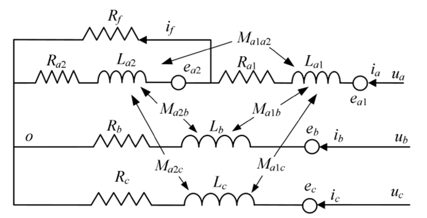
2.1. Mathematical Model of PMSM under Interturn Short-Circuit Fault

The equivalent diagram of PMSM under the inter-turn short-circuit fault is shown in Figure 2. It is assumed that the inter-turn short-circuit fault occurs on the a-phase stator winding of the PMSM. In the figure, a short circuit is added to the a-phase winding of the motor. The short-circuit resistance R f divides the a-phase winding into two parts: a 1 and a 2 , where a 1 represents the normal part, a 2 represents the fault part, and the current i f is the short-circuit current flowing through the resistance R f .
The short-circuit turn ratio is defined as:
u = n N
where n indicates the number of short-circuit turns for the phase stator winding, and N indicates the total number of turns of a phase stator winding.
In the case of an inter-turn short-circuit fault, the voltage equation of PMSM can be expressed as:
V s f = R s f i s f + L s f d i s f d t + e s f + V 0
V s f is defined as:
V s f = R a 1 + R a 2 0 0 R a 2 0 R b 0 0 0 0 R c 0 R a 2 0 0 u R a 1 + R a 2 R f
where V s f denotes the resistance matrix; R f denotes the fault resistance, R a 1 , R a 2 , R b , and R c denote the resistance of stator windings a 1 , a 2 , b , and c , respectively; i s f = i a i b i c i d T denotes the current matrix; i a , i b , and i c denote the stator winding currents of phases a , b , and c , respectively; i f denotes the short-circuit current.
The inductance matrix can be expressed as:
L s f = L a 1 + L a 2 + 2 M a 1 a 2 M a 1 b + M a 2 b M a 1 c + M a 2 c L a 2 M a 1 a 2 M a 1 b + M a 2 b L b M b c M a 2 b M a 1 c + M a 2 c M b c L c M a 2 c L a 2 + M a 1 a 2 M a 2 b M a 2 c L a 2
where L a 1 , L a 2 , L b , and L c denote the self-inductance of stator windings a 1 , a 2 , b , and c , respectively; M j , k indicates the mutual induction between stator windings j and k ( j a 1 , a 2 , b , c and k a 1 , a 2 , b , c ).
The counter electromotive force matrix of the three-phase stator winding and short-circuit winding can be expressed as:
e s f = e a e b e c e d = d d t λ P M , a λ P M , b λ P M , c λ λ P M , f
λ P M , a = λ P M , 1 c o s ( θ ) + ν = 2 k + 1 λ P M , v c o s ( v θ θ v ) λ P M , b = λ P M , 1 c o s ( θ 2 Π 3 ) + ν = 2 k + 1 λ P M , v c o s ( v θ θ v 2 Π 3 ) λ P M , b = λ P M , 1 c o s ( θ + 2 Π 3 ) + ν = 2 k + 1 λ P M , v c o s ( v θ θ v + v 2 Π 3 ) λ P M , b = u λ P M , a
where k Z , λ P M , 1 denotes the fundamental amplitude of the flux linkage; λ P M , v denotes the vth harmonic amplitude of the flux linkage; λ P M , f denotes the flux linkage of the short-circuit winding; θ denotes the rotor electrical angle; θ v denotes the angle between the fundamental and the vth harmonic of the flux linkage; V 0 = V 0 V 0 V 0 0 T denotes the zero-sequence voltage.
The three-phase winding resistance, self-inductance, and mutual inductance of the normal PMSM are equal. The relationship between the short-circuit turn ratio and the resistance, inductance, and back electromotive force in the stator winding can be expressed as:
R a 1 = 1 u R a R a 2 = u R a L a 1 = ( 1 u ) 2 L a L a 2 = u 2 L a
M a 1 a 2 = u 1 u L a M a 2 b = 1 u M a b M a 2 c = 1 u M a c M a 2 b = u M a b M a 2 c = u M a c
λ P M , f = u λ P m , a e f = u e a
When the PMSM suffers from an inter-turn short-circuit fault, its electromagnetic torque can be expressed as:
T e = e a i a + e b i b + e c i c e f i f ω r
where w r denotes the mechanical angular velocity of the rotor of the PMSM, w e denotes the electrical angular velocity of the rotor, and n p denotes the pole pairs of the PMSM.

2.2. Variational Mode Decomposition

VMD is an adaptable signal processing method based on Wiener filtering with VMD, the input signal f t is finally resolved into multiple modal component signals u k ; the unilateral spectrum of each mode u k is obtained by the Hilbert transform, and each mode modulates its corresponding spectrum to the corresponding baseband by adding an exponential term. A confined variational problem is defined as follows:
m i n k t [ ( δ t + j Π t ) · u k t ] e j w k t 2 2
s · t · k u k = f
By using the quadratic punishment factor and the Lagrange multiplier operator λ t , the confined variational problem is transformed into an unconfined variational problem. Then, it is solved by the alternating direction algorithm of multipliers and converted to the frequency domain by Fourier isometric transformation. Finally, the updated expressions of u k n + 1 and w k n + 1 are obtained:
u ^ k n + 1 w = f ^ w i k u ^ i w + ( λ ^ w 2 ) 1 + 2 α ( w w k ) 2
w k n + 1 = 0 w u ^ i w + 2 d w 0 u ^ k w 2 d w

2.3. Constructing Multi-Scale Features

The features extracted by traditional methods cannot efficiently render the state features of the signal, which affects the diagnostic accuracy. Considering the non-stationarity of the signal, the features at a single scale may overlap in the feature space, and it is difficult to fully reveal the signal characteristics. By referring to the multi-scale concept and considering the characteristics of the signal at multiple scales to ensure the overall integrity and local details of the signal, this paper proposes a multi-scale feature index that can reveal the performance of the signal in multi-scale space. Meanwhile, based on the traditional time-domain index, combined with the advantages of multi-scale space on feature space overlap and signal cross-scale complexity, this paper constructs a multi-scale index as the basis for fault classification. Firstly, the time-domain signal is coarse-grained, which makes it difficult to obtain its distribution at different scales. For the time-domain sequence x = x 1 , x 2 , , x n , a signal segmentation of length τ is performed, where the j t h signal segment can be expressed as:
x p , j 1 τ + 1 , x p , j 1 τ + 2 , , x p , j τ , ( 1 j n τ )
The corresponding coarse-grained sequence y τ can be expressed as:
y τ = y 1 τ , y 2 τ , , y j τ , y j τ = 1 τ i = j 1 τ + 1 j τ x i , 1 j n τ
where τ is the scale factor. By extracting the time domain features of the coarse-grained sequence y τ of different scales, the required multi-scale features can be obtained. Since the multi-scale sequence y 1 is the original time-domain sequence x when τ = 1 , the calculated result is the traditional time-domain feature.

2.4. Principal Component Analysis

The principle of PCA is re-linearly combining the high-dimensional variable indexes in the original fault data to construct a new variable index with a lower dimension. These low-dimensional variable indicators are orthogonal and unrelated to each other. Based on this, the coordinate projection of the data sample on the vector is determined by the difference in the independent variables between the samples. The differences reflected by other vectors are reduced in turn, and these vectors are called main components.
The steps of PCA feature extraction are as follows:
Step 1: Given an input signal matrix X = x i j : x i j R n × m , where each row x i R 1 × m , i = 1 , , n of the matrix indicates an index and each column x j R n × 1 , j = 1 , , m of the matrix represents a sample. The average value of the sample x j can be represented as:
x ¯ j = 1 m j = 1 m x j
Step 2: Let C o be the covariance matrix. The eigenvalues λ i , i = 1 , , n and eigenvectors d i , i = 1 , , n of the covariance matrix C o are calculated.
Step 3: The eigenvalues λ 1 λ 2 λ n are arranged in decreasing order, and the eigenvectors corresponding to the eigenvalues are d i , i = 1 , , n . The accumulative contribution rate ς of the first r principal components can be expressed as:
ς = i = 1 r λ i / i = 1 n λ i
Step 4: If ς 0.80 , construct a matrix E R n × r composed of the corresponding feature vectors. Then, the new sample matrix X can use E = d 1 , d 2 , , d r to map the original bearing vibration signal matrix to a new space
X = E T X
where X R r × m .

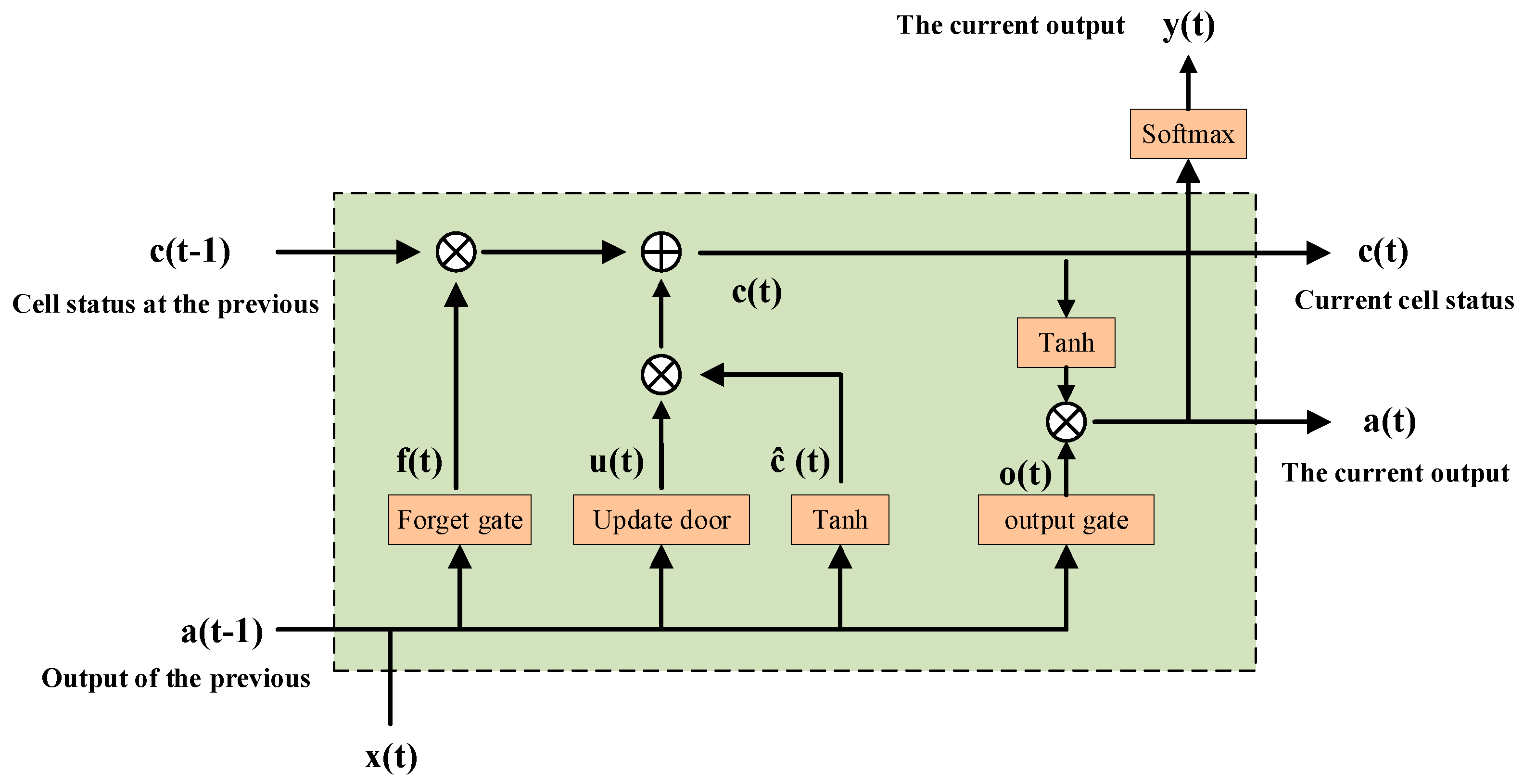
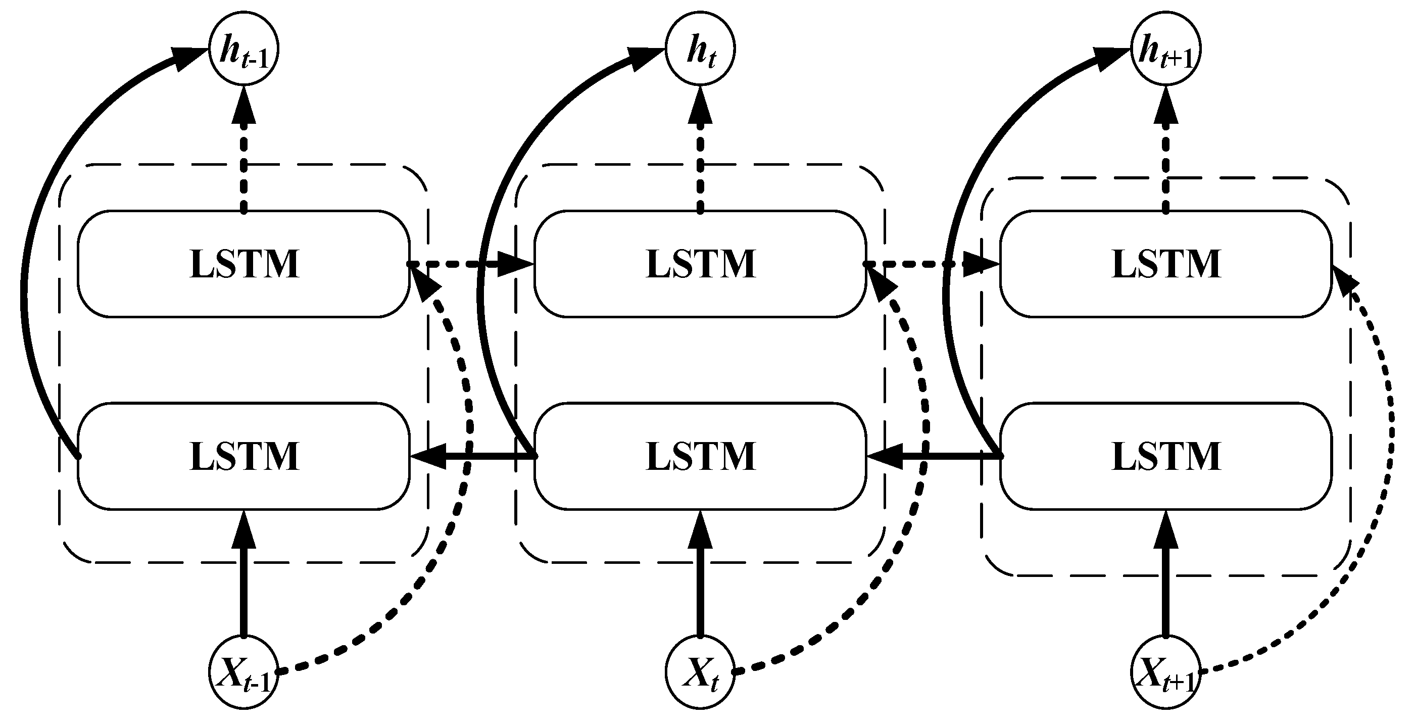
2.5. Long Short-Term Memory Neural Network

The neurons of the LSTM model have a cell state and three gate mechanisms. As shown in Figure 3, the LSTM model has three gates: the forgetting gate, the updating gate, and the output gate, through which the cell state is protected and controlled.
Forgetting door: The sigmoid function determines which information message is discarded, and it can be expressed as:
f t = σ W f a t 1 , x t + b f
where f t is the quantity outgoing to each cell in state c t 1 ; a t 1 is the outgoing at time t 1 ; x t is the intromission at time t ; σ is a sigmoid function, σ x = 1 + e x 1 ; W f is the weight of each variable, and b f is the bias term.
Update door: Update storage information message. First, the sigmoid function calculates the result u t to determine which information message to update. Then, a new candidate value vector c ^ t is generated according to the Tanh function and added to the cell state. By multiplying the old cell state with the forgetting gate f t , part of the old information message is forgotten, u t c ^ t is added, and the current cell state is updated. It can be expressed as:
u t = σ W u a t 1 , x t + b u
c ^ t = t a n h ( W c a t 1 , x t + b c )
c t = u t c ^ t + f t c t 1
where u t 0 , 1 ; tanh outputs a value between −1 and 1; c t 1 is the cell status value at time t 1 ; c ^ t indicates the information message to be extracted from the intromission information at time t, and c t indicates the updated cell status value.
Output gate: Output information message based on the cell status. The sigmoid function determines the quantity of output information. The tanh function processes c t to obtain a value between −1 and 1. o t and c t are multiplied to obtain the output value at time t , which can be expressed as:
o t = σ W o a t 1 , x t + b o
a t = o t t a n h ( c t )
Structurally, compared with the one-way LSTM network, the Bi-LSTM network adopts a two-way loop structure of forward and backward propagation. Viewing the problem from the flow of time, Bi-LSTM adds the data flow from the future into the past based on the one-way flow of LSTM data from the past into the future, and the hidden layer for the past and the hidden layers for the future are independent of each other, so LSTM can better explore the time series feature of data.
The structure of the Bi-LSTM network is shown in Figure 4.
Forward propagation has two steps: (1) move from left to right and calculate from the original time step to the ultimate time step; move from right to left and calculate from the last time step to the ultimate time step. At time step t , the forward layer and the backward layer in the Bi-LSTM use the same input X t , and they jointly generate the output and state. However, the two LSTM network layers do not share the bias vector parameters and weight matrix. The formula can be expressed as:
h t 1 = f W 1 X t + U 1 h t 1
h t 2 = f W 2 X t + U 2 h t + 1
Y t = s o f t   m a x V 1 h t 1 + V 2 h t 2
where f is the hidden-layer activation function; W 1 and W 2 are weight matrix parameters from the intromission layer to the hidden layer; U 1 and U 2 are weight parameters from the hidden layer to the hidden layer, V 1 and V 2 are weight parameters from the hidden layer to the outgoing layer. The weight matrix and bias vector parameters of Bi-LSTM are adjusted by backpropagation according to the error function output by Y t theory.

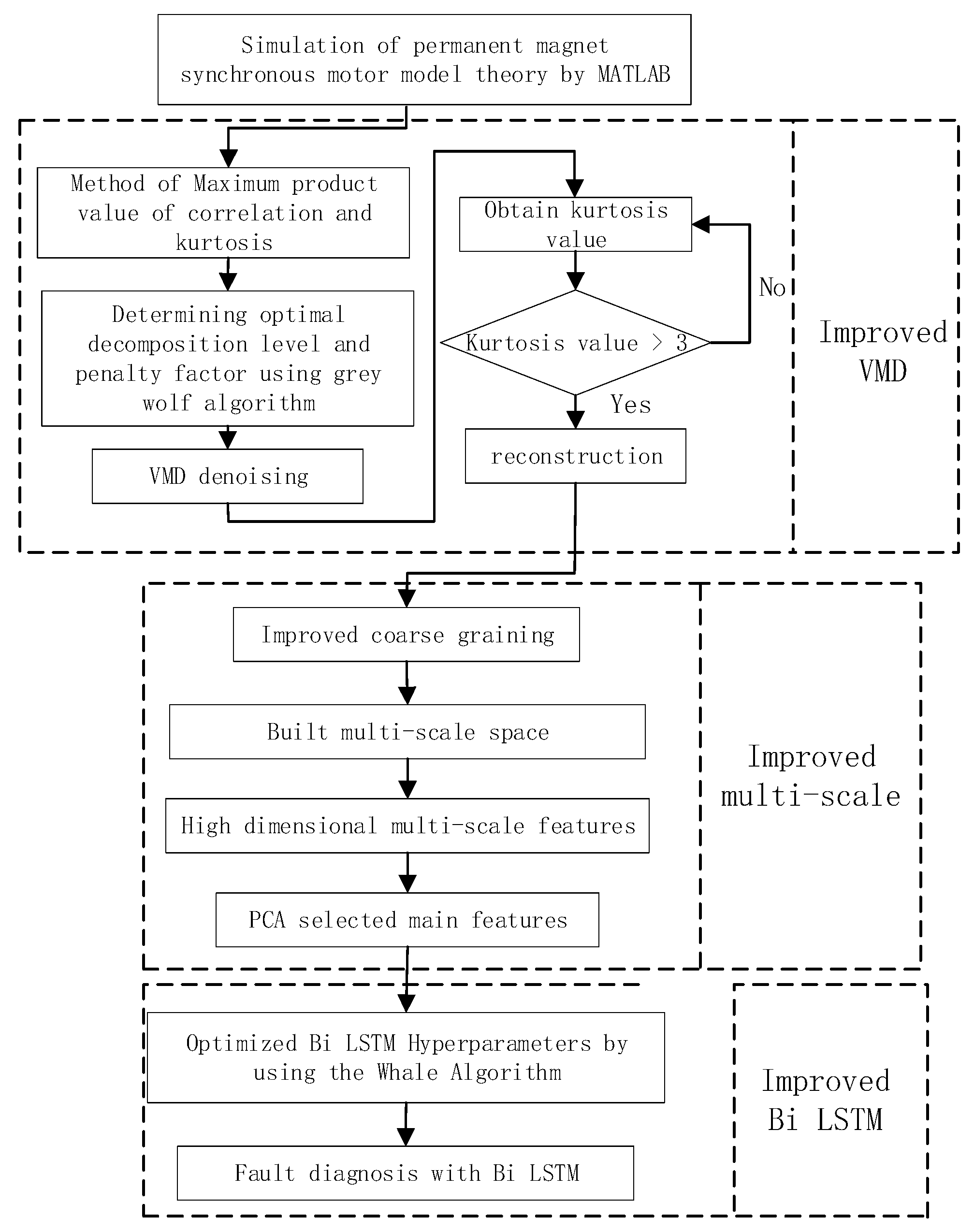
3. The Proposed Method

3.1. Model Optimization of Variational Mode Decomposition

The decomposition order of VMD is determined by the K value. A too-large K value will cause signal decomposition fault, while a too-small K value will lead to incomplete signal decomposition or signal frequency aliasing. The punishment factor α is a key parameter for converting the confined variational problem into an unconfined problem, and it mainly affects the bandwidth of the IMF component obtained by VMD decomposition and the convergence rate of the algorithm. The punishment factor is inversely proportional to the bandwidth of the IMF component. This paper uses the GWO algorithm to optimize K and α .
The GWO algorithm is advanced by observing the grey wolf population’s preying strategy in nature. In the grey wolf group, the grey wolf is classified into four classes from high to low according to the fitness value, which are α wolf, β wolf, δ wolf, and ω wolf. Among them, the α wolf is the optimum result, the β wolf and δ wolf are the second and third optimum results, and the ω wolf is the candidate result. The use of the grey wolf pack predation mechanism to solve the target solution space involves three steps: tracking, encircling, and attacking prey, and they are mapped to the solution to the mathematical model problem, i.e., the fitness from good to bad corresponds to the α wolf, β wolf, and δ wolf in the wolf population, and the other fitness individuals correspond to the ω wolf. The specific algorithm applied to the mathematical model can be represented as:
D = C X p X t
X t + 1 = X p t A D
where D indicates the relative location between the grey wolf and the target; t is the current number of iterations; C and A are coefficients, X p is the location of the target, and X t is the location of the current gray wolf. The values of coefficients C and A are determined by:
C = 2 r 1
A = 2 a r 2 a
a = 2 2 t T m a x
where r 1 and r 2 are random numbers, the value of a linearly reduces from 2 to 0 with the number of iterations t , and T m a x is the maximum number of iterations.
After the gray wolf population completes the positioning and tracking of the prey location, it needs to complete the enclosure of the prey and map it to the mathematical model. The location of ω can be updated by calculating the locations of α , β , and δ . The update formula is represented as:
D α = C 1 · X α X D β = C 2 · X β X D δ = C 3 · X δ X
where D α , D β , and D δ denote the distance between α , β , and δ and the current iterated grey wolf individual; X α , X β , and X δ indicate the current location of α , β , and δ , respectively; C 1 , C 2 , and C 3 are the corresponding coefficients; X denotes the location of the gray wolf individual in the current iteration.
When the prey stops moving, the wolf completes the hunt by attacking. The location of a grey wolf individual can be determined by:
X 1 = X α A 1 · D α X 2 = X β A 2 · D β X 3 = X δ A 3 · D δ
X t + 1 = X 1 + X 2 + X 3 3
where X 1 , X 2 , and X 3 indicate the step length and direction of ω wolves forward to α , β , and δ , respectively; X t + 1 indicates the final location of ω wolves after the iteration.
The maximum value of the product of Pearson correlation p and kurtosis value K v is taken as the optimized objective function value. The specific formula is presented below:
K v = i = 1 N ( X i X ¯ ) 4 4
f m a x = P · K v

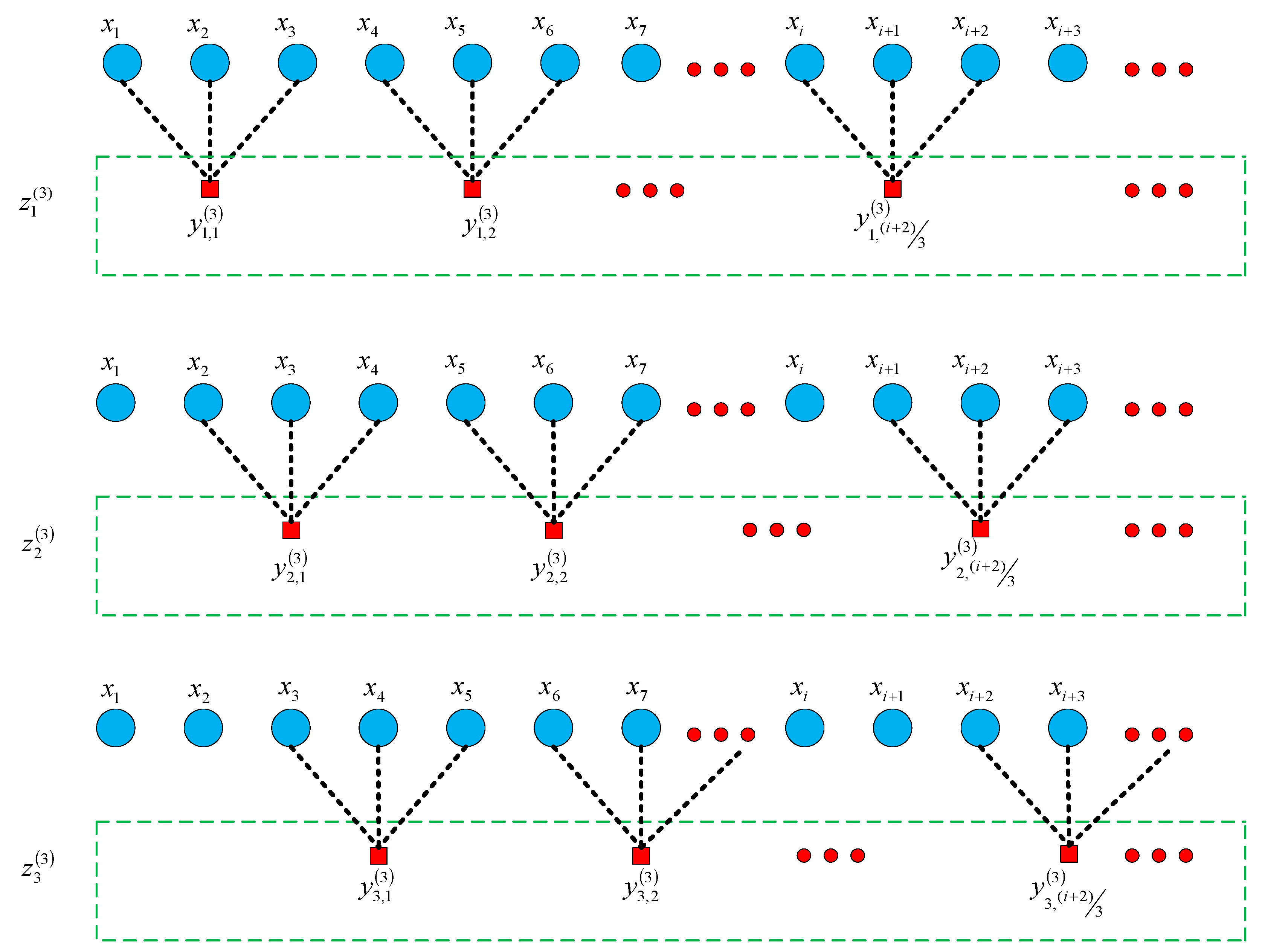
3.2. Multi-Scale Feature Optimization Based on Improved Coarse-Graining

To improve the capability of traditional multi-scale arrangement features, this paper starts with the coarse-grained step and establishes an improved multi-scale feature. Taking scale 3 as an example (as shown in Figure 5), different from the original algorithm, under the same time scale τ , our method can obtain τ sets of time series after coarse-grained processing to solve the mutation problem at the ‘breakpoint’, while there is only one set of time series in the classical algorithm. The mathematical process can be expressed as:
  • The given signal is processed by the improved coarse-grained process to obtain τ sets of time series:
    Z i τ = y i , 1 τ , y i , 2 τ , y i , j τ = f = 0 τ 1 x f + i + τ j 1 τ , i = 1 , 2 , , τ
  • For each set of new coarse-grained time series Z i τ i = 1 , 2 , , τ , its characteristic value in time and frequency domains are obtained, and then the average value of τ time series eigenvalues is calculated to obtain the eigenvalues under the time scale τ .
Figure 5. The time-frequency characteristic method at a scale of 3.
Applsci 13 04064 g005

3.3. Parameter Optimization of Long Short-Term Memory Neural Network

In the process of model training, the optimal set of hyperparameters can be selected to improve the model diagnosis accuracy and performance. The hyperparameters include the number of hidden layers, the learning rate, and the number of hidden layer neurons in the Bi-LSTM prediction model. The hyper-parameter selection of the Bi-LSTM prediction model depends on manual training and is adjusted multiple times according to experience. However, the training of the Bi-LSTM prediction model requires a certain amount of time, which will inevitably decline the work efficiency. Moreover, the hyper-parameter combination of the prediction model selected by this method is not optimal, which will affect the accuracy and effectiveness of the prediction model. To address this issue, the whale algorithm is employed to optimize the hidden layer neural network and learning rate of the Bi-LSTM fault model to enhance the generalization capability and estimation accuracy of the model.
The whale algorithm is a mathematical model developed by based imitating the behaviors of humpback whales to surround, dabble, and search for prey. It has the advantages of less parameter adjustment, simple operation, and a strong ability to jump out of local optima.
The first stage is:
D = C · X t X t
X t + 1 = X t A · D
where D denotes the distance vector between the current optimal solution and the search body; t denotes the current iteration times; X denotes the location vector of the current optimal solution; X denotes the location vector of the search volume.
The second stage is:
X t + 1 = D · e b l · c o s ( 2 Π l ) + X t
where D = X t X t denotes the distance vector between the searching individual and the target prey; b denotes the constant coefficient of logarithmic spiral shape; l denotes a random number in the interval 1 ,   1 .
The third stage is:
D = C · X r a n d X t
X t + 1 = X r a n d A · D
where X r a n d denotes the location of a random search body in the current population.
The flowchart of using the whale algorithm to optimize the hyperparameters of the Bi-LSTM diagnostic model is shown in Figure 6.

4. Experiments and Results

Firstly, the experimental data are obtained by the Simulink simulation program in MATLAB, and the collected data are sorted out. Secondly, the effectiveness of the improved method is verified by ablation experiments and comparative analysis.

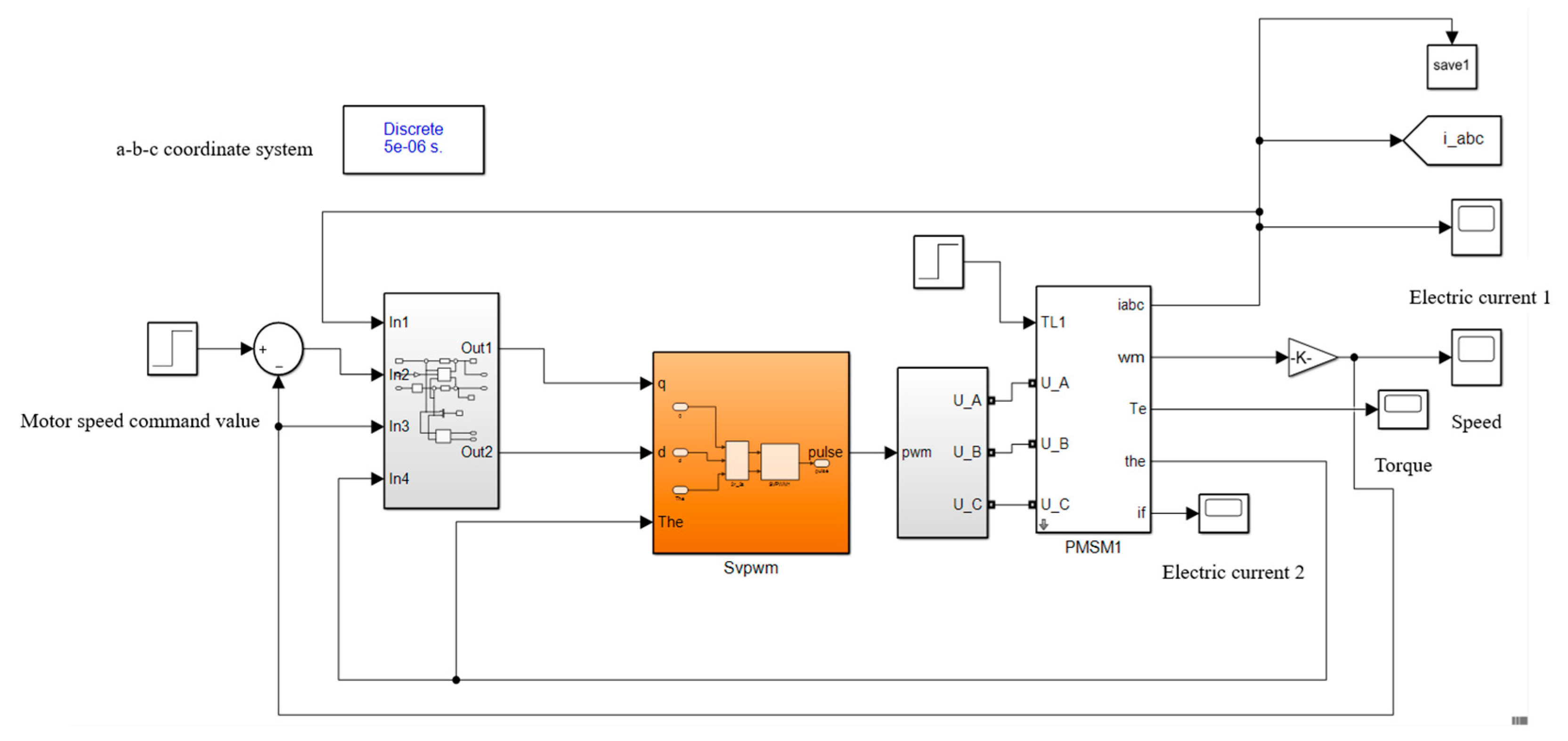
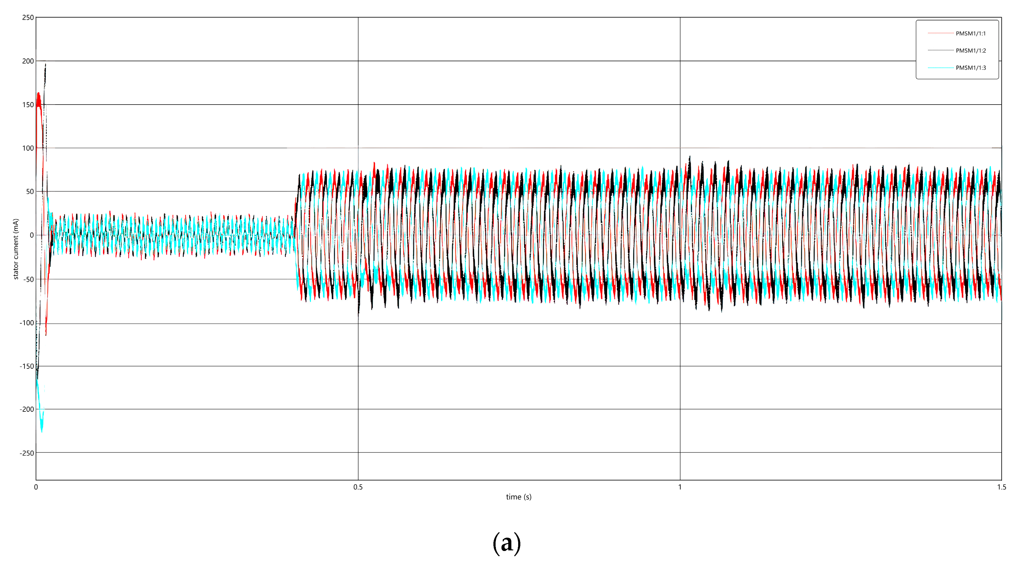
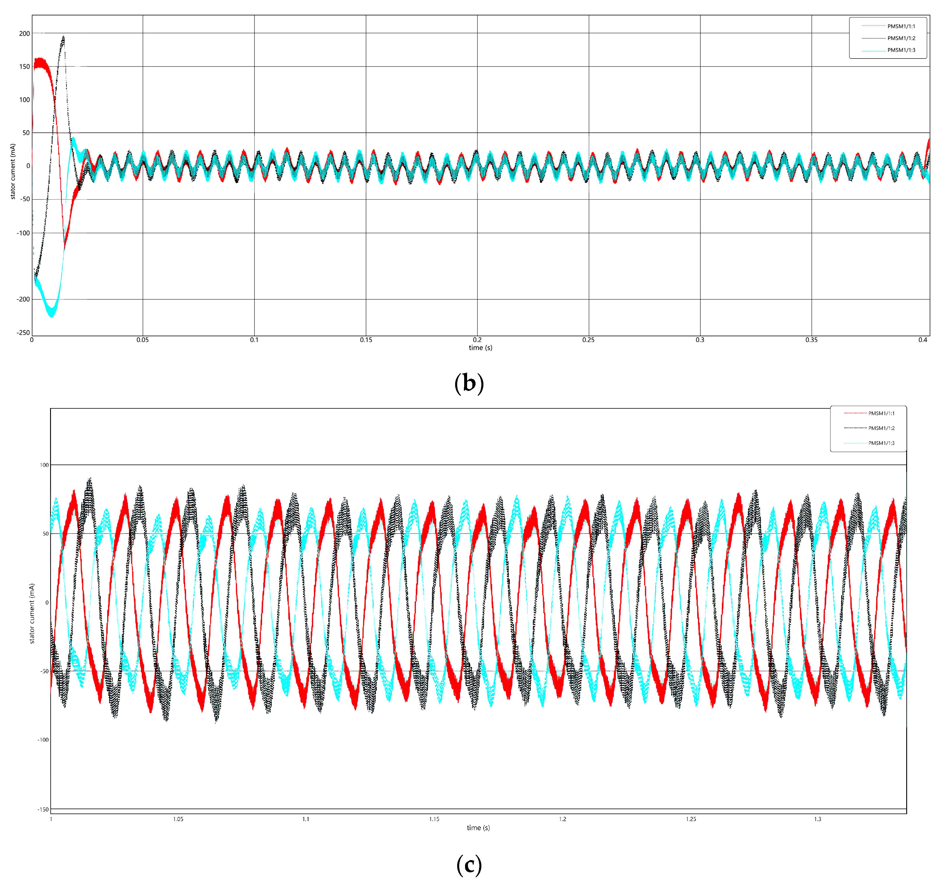
4.1. Data Acquisition

Through the Simulink in MATLAB, it is simulated that the inter-turn short-circuit fault occurs in the a-phase stator winding after the PMSM runs normally for 0.5 s. The simulation model is shown in Figure 7. The stator current waveform is shown in Figure 8. Figure 8a presents the stator current simulation diagram of the permanent magnet synchronous motor from start-up to normal operation to the occurrence of inter-turn short circuit fault. Figure 8b presents the local amplification diagram of 0.4 s before the period in Figure 8a. Figure 8c is the local amplification diagram of 1 s after the period in Figure 8a. It can be seen from Figure 8b that under normal circumstances, the three-phase current is a periodic waveform. In this paper, phase a stator current is selected as the fault feature to detect the occurrence of a fault.
Under normal circumstances, there is no short-circuit current in the PMSM, so its value is zero; after an inter-turn short-circuit fault occurs, a short-circuit loop is generated, thereby generating a short-circuited current. The above simulation results show that the stator current of the PMSM changes significantly after the inter-turn short-circuit fault occurs.

4.2. Ablation Experiments

4.2.1. The Effectiveness of the VMD Algorithm Based on GWO Optimization

This paper proposes a VMD decomposition method based on GWO optimization to remove noise in the signal. By comparing the results of inter-turn short circuit fault diagnosis using the improved VMD decomposition method with those using the traditional VMD decomposition method, the effectiveness of the improved algorithm is verified. It should be noted that the feature extraction part adopts the unimproved multi-scale feature extraction method, and the fault diagnosis part adopts the unimproved Bi-LSTM neural network model.
Since no failure occurs in the first 0.5 s of the dataset, it was deleted. Then, 300 sets of data are collected for each of the five faults, with 2000 data in each group. The sample data of the training dataset and the test dataset are obtained by dividing each fault sample by a ratio of 5:1. For the VMD decomposition method based on GWO optimization, the initial population of the GWO algorithm is set to 20, and the maximum number of iterations is 10. The decomposition number and punishment factors are selected in the ranges of 2 ,   12 and 1000 ,   3000 . Finally, the optimized IMF decomposition number K = 6 , and the punishment factor α = 1564 .
The training set is tested by the trained model, and then the results are compared with the original results. Finally, the ratio of the predicted correct value to the total number is calculated to obtain the correct rate of the training set, as shown in Figure 9. Figure 9a presents the result of using the unimproved VMD decomposition method, and Figure 9b presents the result of using the improved VMD decomposition method. It can be seen from the figure, the accuracy of the model before VMD improvement becomes stable after 1200 iterations, and the accuracy of the model after VMD improvement becomes stable after 1000 iterations.
Figure 10 shows the confusion matrix of the fault classification model on the test set in the experiment. Figure 10a presents the confusion matrix of using the unimproved VMD decomposition method, and Figure 10b presents the confusion matrix of using the improved VMD decomposition method. It can be seen from Figure 10 that for fault category 2, both the unimproved and improved models can make a correct diagnosis. For fault category 1, both the unimproved and the improved VMD make three diagnostic errors. For fault category 3, both the unimproved and improved VMD make one diagnostic error. For fault category 4, the unimproved VMD makes four diagnostic errors, while the improved VMD makes three diagnostic errors. For fault category 5, the unimproved VMD makes nine diagnostic errors, while when the improved VMD makes six diagnostic errors. The final fault identification accuracy of the two methods is 93.2% and 94.8% respectively.
The t-SNE method is used to obtain the 2D scatter plot, which can demonstrate the fault classification effect more intuitively, as shown in Figure 11. Figure 11a presents the 2D scatter plot using the unimproved VMD decomposition method, and Figure 11b presents the 2D scatter plot using the improved VMD decomposition method. The results in Figure 11 indicate that the distance between and within the VMD classes before and after the improvement is not very different, and the effect is not good.

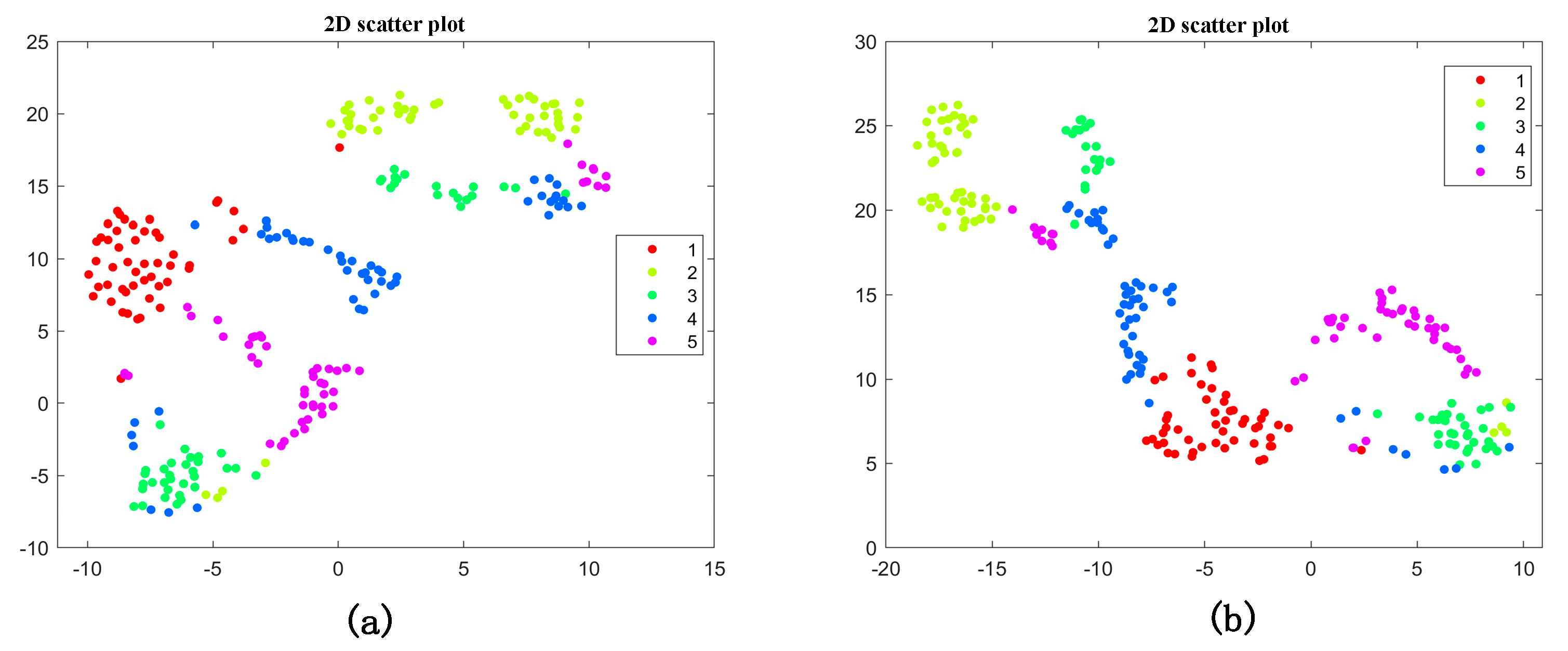
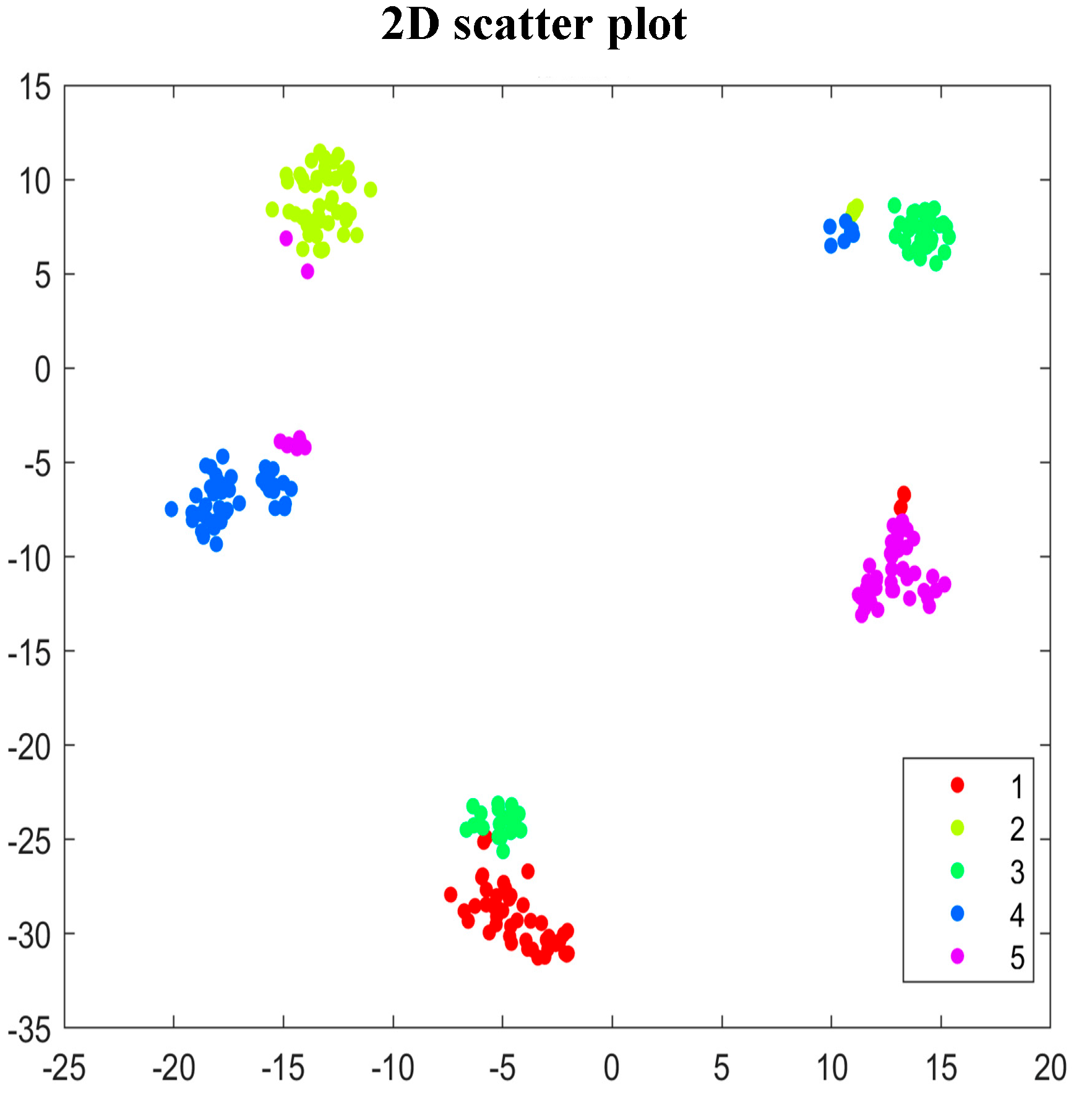
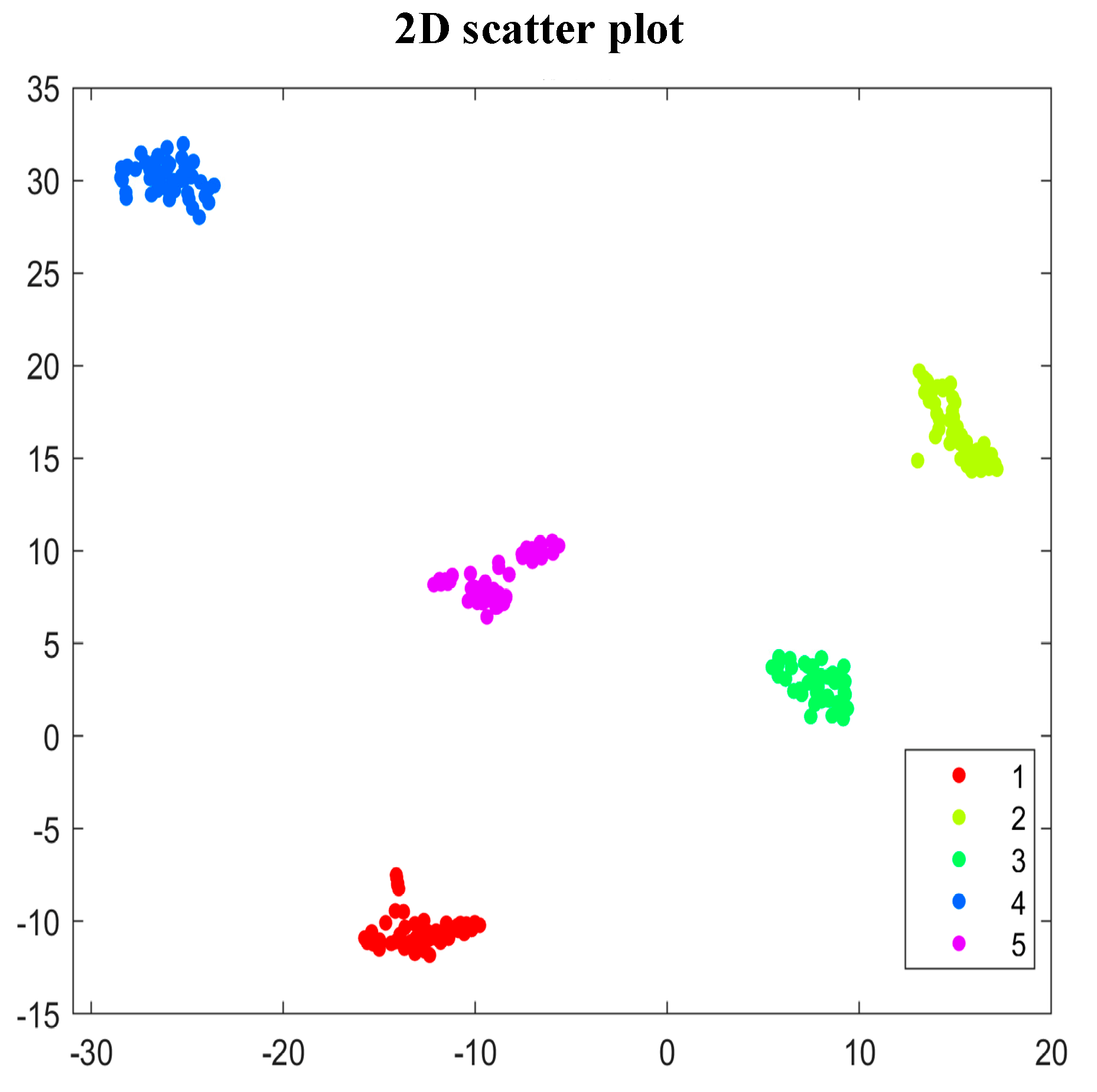
4.2.2. The Effectiveness of the Improved Coarse-Grained Multi-Scale Feature Extraction Method

In this paper, an improved coarse-grained multi-scale feature extraction method is proposed. The reconstructed signal is processed by improved coarse-grained processing at different scales. The effectiveness of the improved algorithm is verified by comparing the results of inter-turn short circuit fault diagnosis using the improved multi-scale feature extraction method with those of using the traditional multi-scale feature extraction method. It should be noted that the data preprocessing part adopts the improved VMD decomposition method, and the fault diagnosis part adopts the unimproved Bi-LSTM neural network model.
After the decomposed signal is obtained by the improved VMD decomposition method, the decomposed signal is reconstructed. The decomposed signal is reconstructed by kurtosis value, and the decomposed components with more impact information can be screened out. Table 1 shows the kurtosis values of six signals decomposed by VMD from three samples for each of the five faults. In reference [18], the decomposition signal with a kurtosis value greater than 3 is superimposed and reconstructed. The reconstructed signal is subjected to different scales of improved coarse-grained processing to obtain its distribution at different scales of 1–10. For each new set of coarse-grained time series, its time-frequency domain eigenvalues are obtained, and then the average value of the eigenvalues of τ time series is calculated. The 19 time-frequency domain eigenvalues under the time scale τ can be obtained. There are 14 time domains, which are the maximum value, minimum value, average value, peak-peak value, average value of absolute value, variance, standard deviation, kurtosis, skewness, root mean square, waveform factor, peak factor, pulse factor, and margin factor. There are five frequency domains, which are the center of gravity frequency, mean square frequency, root mean square frequency, frequency variance, and frequency standard deviation. Each scale has 19 features, and there are 190 features in 10 scales. The PCA was used to extract the main features and normalize them by the Map minmax function.
Figure 12, Figure 13 and Figure 14 show the training set accuracy, confusion matrix, and 2D scatter plot obtained by using the improved multi-scale feature extraction method for inter-turn short circuit fault diagnosis.
Comparing Figure 12 with Figure 11b, it can be seen that the accuracy of the unimproved ordinary time-frequency domain feature extraction model tends to be stable after 1000 iterations, and the accuracy of the improved multi-scale time-frequency domain feature extraction model tends to be stable after 800 iterations. Comparing Figure 13 with Figure 12b, it can be seen that for fault category 2, the model can make a correct diagnosis. For fault category 1, the model based on ordinary time-frequency domain feature extraction makes three diagnostic errors, and the model based on improved multi-scale feature extraction makes two diagnostic errors. For fault category 3, the model based on ordinary time-frequency domain feature extraction makes one diagnostic error, and there is no error after using the improved multi-scale feature extraction. For fault category 4, both methods make three diagnostic errors. For fault category 5, the model based on ordinary time-frequency domain feature extraction makes six diagnostic errors, and the model based on multi-scale feature extraction makes four diagnostic errors. The final fault identification accuracy of the two methods is 94.8% and 96.4%, respectively. By comparing Figure 14 with Figure 13b, it can be seen that the improved multi-scale time-frequency domain feature extraction model has a larger inter-class distance and smaller intra-class distance, which does not achieve the desired effect.

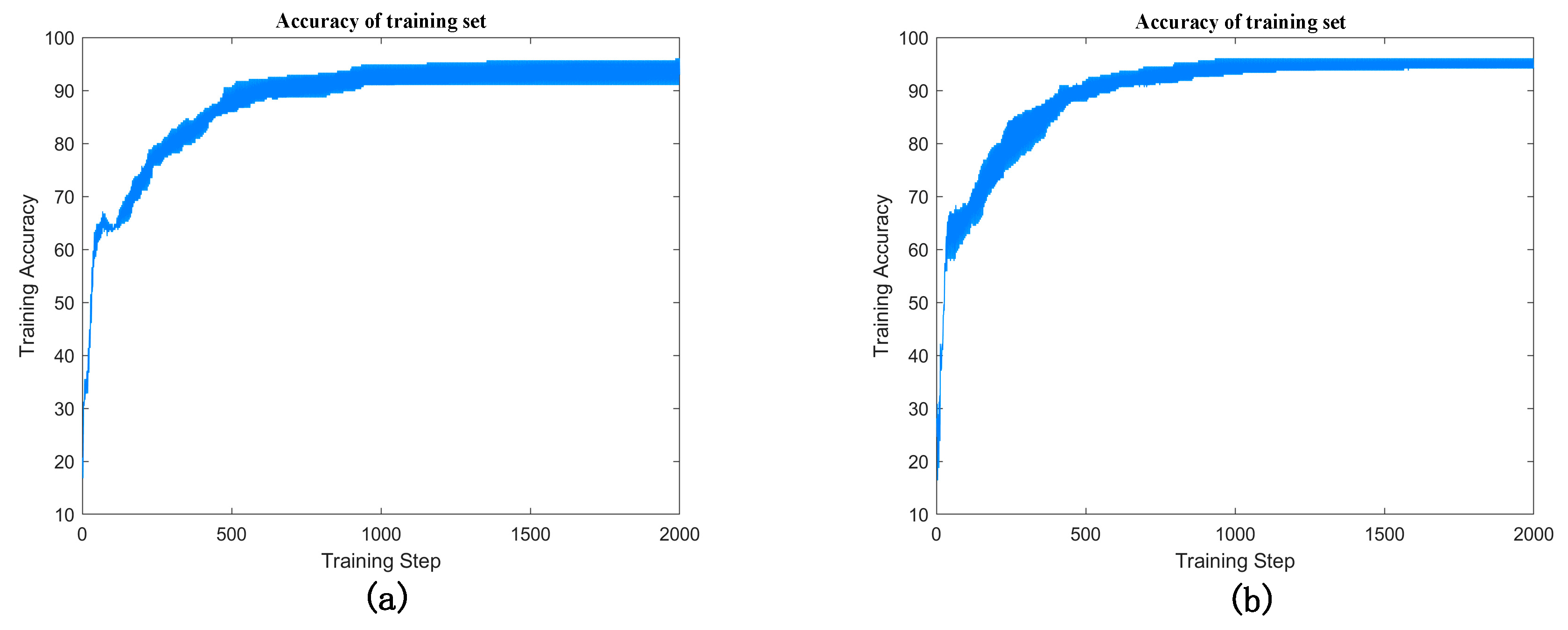
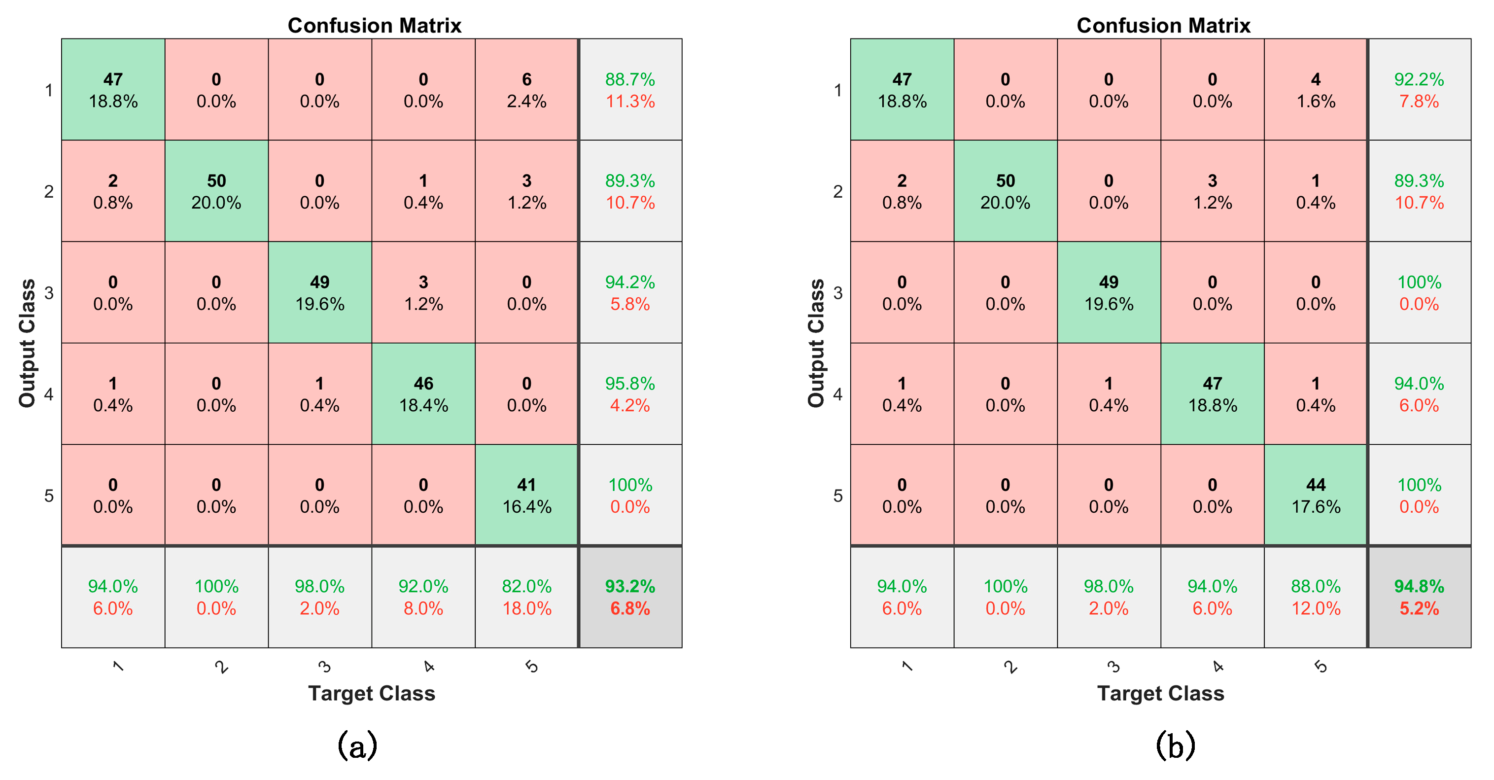
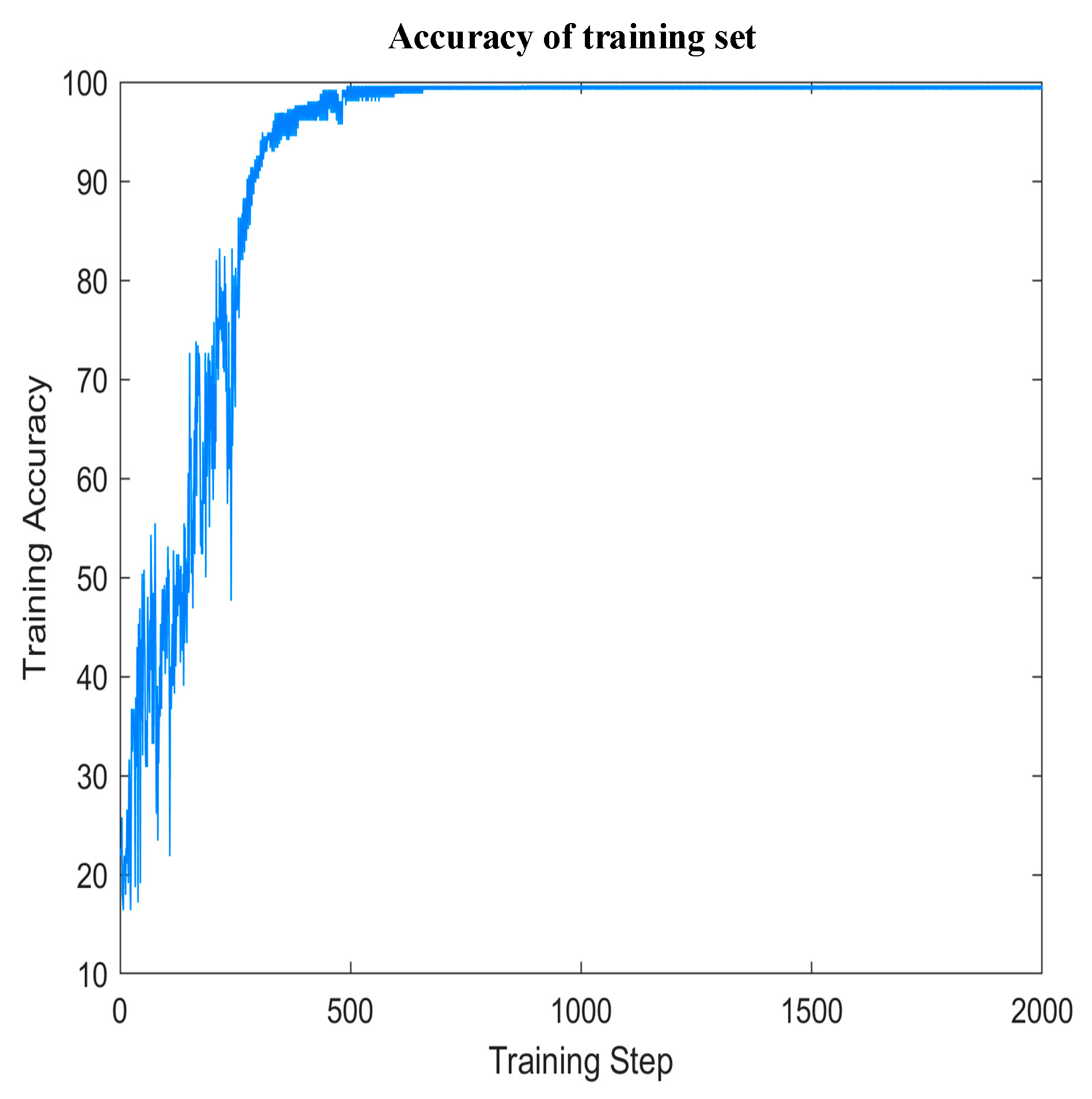
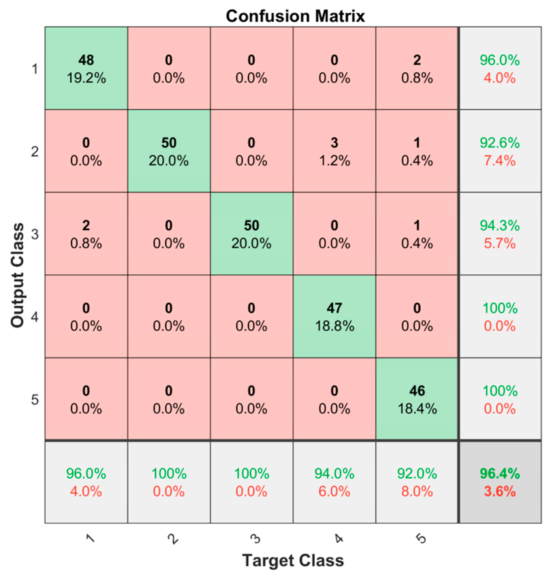
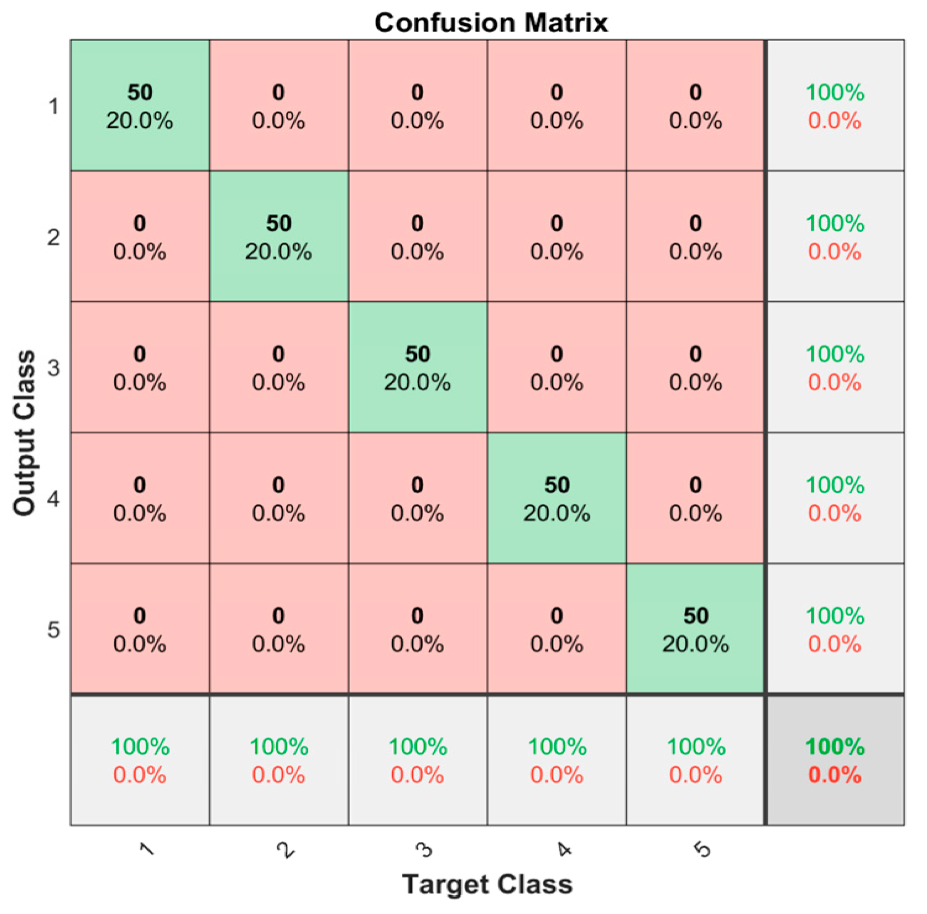
4.2.3. The Effectiveness of the Fault Diagnosis Model Based on the Improved Bi-LSTM Neural Network

In this paper, a Bi-LSTM neural network model based on WOA optimization is proposed to realize the fault diagnosis of inter-turn short circuits. By comparing the fault diagnosis results of the improved Bi-LSTM neural network with those of the unimproved Bi-LSTM neural network, the effectiveness of the improved algorithm is verified. It should be noted that the data preprocessing part adopts the improved VMD decomposition method, and the feature extraction part adopts the improved multi-scale feature extraction method.
The number of hidden-layer nodes and learning rate in the Bi-LSTM prediction model are hyperparameters. During model training, the diagnosis accuracy and performance of the model can be improved by selecting the best set of hyperparameters through hyperparameter optimization. The WOA optimization algorithm is used to optimize the number of hidden layer nodes and the learning rate of the Bi-LSTM network to reduce the diagnostic error. The LSTM network has one hidden layer and one fully connected layer. The selection ranges of the number of hidden-layer nodes and the learning rate parameter are 100 ,   300 and 0.001 ,   1 , respectively. The population and iteration times of the whale algorithm are 10 and 50, respectively.
Figure 15, Figure 16 and Figure 17 show the accuracy of the training set, the confusion matrix, and the 2D scatter plot obtained by using the improved Bi-LSTM neural network for inter-turn short circuit fault diagnosis.
Comparing Figure 12, Figure 13 and Figure 14, it can be seen that the improved VMD decomposition method, the improved multi-scale feature extraction method, and the improved Bi-LSTM fault diagnosis model have been greatly improved in all aspects. It can be seen from the whole training iteration process that the accuracy of the model tends to be stable after 300 iterations. The accuracy of fault identification is as high as 100%, the distance between classes becomes larger, the distance within classes becomes smaller, and it has high accuracy and robustness. The proposed fault diagnosis model based on multi-scale space can effectively classify PMSM inter-turn short circuit faults of different degrees.

5. Conclusions and Future Works

In this paper, the inter-turn short circuit fault simulation program of PMSM is designed, and the stator current data is collected by the Simulink simulation program. Then, the inter-turn short circuit fault diagnosis model of the permanent magnet synchronous motor based on multi-scale space is proposed. The experimental results indicate that the proposed method achieves a good diagnosis effect for different degrees of inter-turn short circuit fault of the permanent magnet synchronous motor, and the fault diagnosis accuracy is as high as 100%. The conclusions of this paper are as follows.
  • The GWO algorithm is used to adaptively select the k value and α value in VMD decomposition, and the maximum value of the product of Pearson correlation p and kurtosis value K v is taken as the optimized objective function value, to realize the extraction of weak signals in inter-turn short circuit faults.
  • The improved coarse-grained multi-scale feature extraction improves the performance of traditional multi-scale arrangement features.
  • The WOA is adopted to optimize the number of hidden-layer nodes and the learning rate of the Bi-LSTM network, which improves the diagnostic accuracy and solves the problem of the hyper-parameter configuration of the deep learning model.
  • In practical engineering applications, a new fault diagnosis method is proposed to make fault diagnosis more intelligent.
This paper only studies the stator winding inter-turn short circuit fault of PMSM. In the future, we will conduct more extensive experimental research on other fault types of PMSM, expand the data set, and apply this fault diagnosis method to actual industrial production.

Author Contributions

Conceptualization, F.M.; methodology, F.M., L.Q. and S.Y.; software, F.M., L.Q. and S.Y.; validation, Y.C., H.X. and S.L.; data curation, L.Q. and S.Y.; writing—original draft preparation, F.M.; writing—review and editing, F.M., L.Q. and S.Y.; visualization, F.M.; project administration, L.Q. and S.Y.; funding acquisition, L.Q. and S.Y. All authors have read and agreed to the published version of the manuscript.

Funding

General Projects of National Natural Science Foundation of China (Project number: 51875270), Industry—University Research Project of Jiangsu (Project number: No. BY2020031), Graduate In-novation Program (Project number: SJCX22_1887).

Institutional Review Board Statement

Not applicable.

Informed Consent Statement

Not applicable.

Data Availability Statement

Data is unavailable due to privacy or ethical restrictions.

Conflicts of Interest

The authors declare no conflict of interest.

References

  1. Hu, Y. Model Predictive Torque Control Strategy for Marine Permanent Magnet Synchronous Propulsion Motor. Master’s Thesis, Wuhan University of Technology, Wuhan, China, 2019. (In Chinese). [Google Scholar]
  2. Yu, C.; Qi, L.; Sun, J.; Jiang, C.; Su, J.; Shu, W. Fault diagnosis technology for ship electrical power system. Energies 2022, 15, 1287. [Google Scholar] [CrossRef]
  3. Zhang, H.; Liu, Y.; Zhao, X.; Hu, Q.; Liu, D. Fuzzy wavelet network intelligent predictive controller for vacuum injection molding. Comput. Integr. Manuf. Syst. 2010, 16, 2647–2652. (In Chinese) [Google Scholar]
  4. Zhang, L.; Yang, M. Fault diagnosis of permanent magnet synchronous motor based on mixup-LSTM. Electr. Switch. 2022, 60, 58–62. (In Chinese) [Google Scholar]
  5. Xue, S.; He, Q.; Pan, J.; Huang, X. Research on dynamic eccentricity fault diagnosis method of permanent magnet synchronous motor based on GA-SVM. Zuhe Jichuang Yu Zidonghua Jiagong Jishu 2022, 99–103. (In Chinese) [Google Scholar]
  6. Zhao, S.; Song, Q.; Zhang, Y.; Zhang, W. Mechanical fault detection of permanent magnet synchronous motor based on improved DFA and LDA. J. Beijing Inst. Technol. 2023, 43, 61–69. (In Chinese) [Google Scholar]
  7. Huang, W.; Du, J.; Hua, W.; Fan, Q. An open-circuit fault diagnosis method for PMSM drives using symmetrical and DC components. Chin. J. Electr. Eng. 2021, 7, 124–135. [Google Scholar] [CrossRef]
  8. Tang, S.; Chen, X.; Zheng, S. Fault diagnosis method of motor bearing based on attention and multi-scale convolution neural network. Electr. Technol. 2020, 21, 32–38. (In Chinese) [Google Scholar]
  9. Li, F.; Honglin, L.; Shuiqing, X. Research on open circuit fault diagnosis of PMSM Inverter with SDAE-FFNN network. Chongqing Ligongxue Xuebao 2013, 1–9. (In Chinese) [Google Scholar]
  10. Chen, Z.; Liang, K.; Peng, T.; Wang, Y. Multi-condition PMSM fault diagnosis based on convolutional neural network phase tracker. Symmetry 2022, 14, 295. [Google Scholar] [CrossRef]
  11. Zhang, Y.; Lei, Y. Data anomaly detection of bridge structures using convolutional neural network based on structural vibration signals. Symmetry 2021, 13, 1186. [Google Scholar] [CrossRef]
  12. Lee, H.; Jeong, H.; Kim, S.W. Detection of interturn short-circuit fault and demagnetization fault in IPMSM by 1-D convolutional neural network. In Proceedings of the 2019 IEEE PES Asia-Pacific Power and Energy Engineering Conference (APPEEC), Macao, China, 1–4 December 2019; pp. 1–5. [Google Scholar]
  13. Man, Y.; Yang, L.; Yan, L.; Cui, G. Detection method of incipient inter-turn short circuit fault of PMSM based on VMD. Electr. Mechines Control Appl. 2022, 49, 66–74. (In Chinese) [Google Scholar]
  14. Wang, Y. Fault Diagnosis of Interturn Short Circuit in Permanent Magnet Synchronous Motor Based on Stacked Sparse Autoencoder. Master’s Thesis, Jiangsu University of Science and Technology, Zhenjiang, China, 2021. (In Chinese). [Google Scholar]
  15. Gu, J.; Jiang, T.; Zhu, H. Multi-objective discrete grey wolf optimization algorithm for job shop energy saving scheduling. Comput. Integr. Manuf. Syst. 2021, 27, 2295–2306. (In Chinese) [Google Scholar]
  16. Xu, F.; Fang, Y.; Zhang, R. Cluster fault diagnosis of PCA-GG rolling bearing based on EEMD fuzzy entropy. Comput. Integr. Manuf. Syst. 2016, 22, 2631–2642. (In Chinese) [Google Scholar]
  17. Liu, J.; Ma, Y.; Li, Y. Improved whale algorithm for solving engineering design optimization problems. Comput. Integr. Manuf. Syst. 2021, 27, 1884–1897. (In Chinese) [Google Scholar]
  18. Wang, J.; Li, F. Review of signal processing methods in fault diagnosis for machinery. Noise Vib. Control. 2013, 33, 128–132. (In Chinese) [Google Scholar]
Figure 1. The diagnosis process of the proposed method.
Applsci 13 04064 g001
Figure 2. PMSM equivalent model of a phase inter-turn short-circuited fault.
Applsci 13 04064 g002
Figure 3. The structure of the LSTM model.
Applsci 13 04064 g003
Figure 4. The structure of the Bi-LSTM network.
Applsci 13 04064 g004
Figure 6. The flowchart of using the whale algorithm to optimize the hyperparameters of the Bi-LSTM diagnostic model.
Applsci 13 04064 g006
Figure 7. The simulation diagram of the permanent magnet synchronous motor a phase stator winding inter-turn short-circuit.
Applsci 13 04064 g007
Figure 8. (a) The waveform of the stator current signal. (b) The stator current. (c) The simulation of the stator current with a short-circuit turn ratio of 0.2.
Applsci 13 04064 g008aApplsci 13 04064 g008b
Figure 9. The accuracy in the training process. (a) The accuracy in the training process by unimproved VMD. (b) The accuracy in the training process by improved VMD.
Applsci 13 04064 g009
Figure 10. The confusion matrix. (a) The confusion matrix in the training process by the unimproved VMD. (b) The confusion matrix in the training process by the improved VMD.
Applsci 13 04064 g010
Figure 11. The 2D scatter plot. (a) The 2D scatter plot in the training process by the unimproved VMD. (b) The 2D scatter plot in the training process by the improved VMD.
Applsci 13 04064 g011
Figure 12. The accuracy of the training set using the improved multiscale feature extraction.
Applsci 13 04064 g012
Figure 13. The confusion matrix of using the improved multiscale feature extraction.
Applsci 13 04064 g013
Figure 14. The 2D scatter plot using the improved multiscale feature extraction.
Applsci 13 04064 g014
Figure 15. The accuracy of the training set using the improved Bi-LSTM network.
Applsci 13 04064 g015
Figure 16. The confusion matrix using the improved Bi-LSTM network.
Applsci 13 04064 g016
Figure 17. The 2D scatter plot using the improved Bi-LSTM network.
Applsci 13 04064 g017
Table 1. The kurtosis values of five faults after VMD.
Failure ModeSample LabelKurtosis Value after VMD
1S16.241.5225.711.5323.658.96
S23.183.381.5212.871.5123.94
S33.423.081.5212.381.5216.32
2S43.053.401.5212.131.5129.16
S52.891.5222.571.5424.0813.42
S62.981.5320.101.5420.9116.10
3S73.033.391.5311.951.5231.91
S83.442.981.5311.971.5238.54
S93.462.811.5311.441.5230.73
4S103.571.5319.021.5515.5521.01
S113.181.5317.951.5516.8719.15
S123.023.361.5312.251.5221.24
5S135.201.5252.689.031.5421.00
S146.421.5348.699.231.5420.98
S152.381.5354.719.051.5421.98
Disclaimer/Publisher’s Note: The statements, opinions and data contained in all publications are solely those of the individual author(s) and contributor(s) and not of MDPI and/or the editor(s). MDPI and/or the editor(s) disclaim responsibility for any injury to people or property resulting from any ideas, methods, instructions or products referred to in the content.

