A Deep Learning Framework for Day Ahead Wind Power Short-Term Prediction

Abstract

Due to the increasing proportion of wind power connected to the grid, day-ahead wind power prediction plays a more and more important role in the operation of the power system. This paper proposes a day-ahead wind power short-term prediction model based on deep learning (DWT_AE_BiLSTM). Firstly, discrete wavelet transform (DWT) is used to denoise the data, then an autoencoder (AE) technology is used to extract the data features, and finally, bidirectional long short-term memory (BiLSTM) is used for prediction. To verify the effectiveness of the proposed DWT_AE_BiLSTM model, we studied three different power stations and compared their performance with the shallow neural network model. Experimental analysis shows that this model is more competitive in forecasting accuracy and stability. Compared with the BP model, the proposed model has increased by 3.86%, 3.22% and 3.42% in three wind farms, respectively.

1. Introduction

In the past few decades, the scale of wind power generation has rapidly increased. As reported by the Global Wind Energy Council (GWEC), the cumulative installed capacity of global wind energy reached 743 GW at the end of 2020 [1], an increase of 59% compared to 2019. Due to the random, nonlinear and nonstationary characteristics of wind energy, this rapid growth has led to a series of problems, such as the instability of power system balance and control [2]. More and more studies reveal that accurate short-term wind power prediction is helpful in optimizing scheduling and energy trading [3,4].

The majority of scholars classify wind power forecasting methods into four categories: physical models, statistical models, machine-learning models and hybrid models [5,6,7]. Physical models are based on geographic environments and numerical weather forecasts (NWFs), such as wind speed, wind direction, temperature, humidity and pressure of 1–3 days, in advance. However, it requires rich expert experience and complex computation. It is mainly applicable to new power stations without historical data. The statistical model depends on the historical data observed by the power station to forecast future power generation, mainly using multiple regression methods, such as the Kalman filter [8], moving average (MA) methods, autoregressive (AR) or autoregressive moving average model (ARMA) [9,10].

In recent years, machine-learning methods have been extensively studied and applied to short-term wind power forecasts, such as the support vector machine (SVM) [11,12], random forest (RF) [13] and so on. Ding et al. proposed a time series model based on a hybrid-kernel least-squares support vector machine [11], and Lahour et al. presented a model based on random forests for hour-ahead wind power forecast [13].

With the flourishing of artificial intelligence techniques, deep learning models with strong nonlinear complex mapping abilities are becoming more and more popular. Such as the deep belief network (DBN) [14,15]. Yu et al. proposed a bidirectional recurrent neural network (RNN)-based encoder-decoder scheme to learn efficient and robust embeddings for a high-dimensional multivariate time series [16]. Liu et al. proposed a stacked recurrent neural network (SRNN) based on a parameter sine activation function (PSAF) for wind power prediction [17] using a convolutional neural network (CNN) [18] and long short-term memory (LSTM) [19]. Liu et al. used a convolution neural network and long short-term memory for power prediction, and used a genetic algorithm to optimize the model [20]. Yin et al. applied a quadratic mode decomposition and cascade deep learning to ultrashort-term wind power prediction [21]. Lawal et al. used a one-dimensional convolution neural network (CNN) and bidirectional short-term memory (BLSTM) networks to predict short-term wind speed at different heights [22]. Wang et al. proposed a deep belief network (DBN) model for regression with an architecture of 144 input and 144 output nodes and was constructed using a restricted Boltzmann machine (RBM) [14]. Higashiyama et al. explored the feature extraction scheme based on three-dimensional convolutional neural networks (3D-CNNs) [18]. Qu et al. showed a wind power prediction model based on the long short-term memory model [19].

In order to absorb the advantages of each model prediction method, some hybrid model methods are proposed. Wang et al. [23] designed a new Laguerre neural network to build the hybrid forecasting model optimized by the opposition transition state transition algorithm. Viet et al. [24] proposed a combined artificial neural network model with a particle swarm optimization algorithm and genetic algorithm.

However, these statistical and machine learning methods are data-driven and limited by the data quality of the training set, so it is difficult to further improve the prediction accuracy. The data collected from the wind farm is large, but there may be redundancy among the data. Most previous studies have ignored this problem. Autoencoder is used to discover more abstract, high-level hidden features. By using sparse features, the dimension of the original data is reduced, and the representative information is retained to improve the robustness of the algorithm and the accuracy of the prediction.

Based on the above considerations, this paper presents a deep learning day-ahead wind power prediction framework based on discrete wavelet transform, sparse feature extraction and bidirectional deep learning. The main contributions of this paper are as follows:

(a)

According to the characteristics of wind power forecasting, a deep learning framework DWT_AE_BiLSTM is first proposed.

(b)

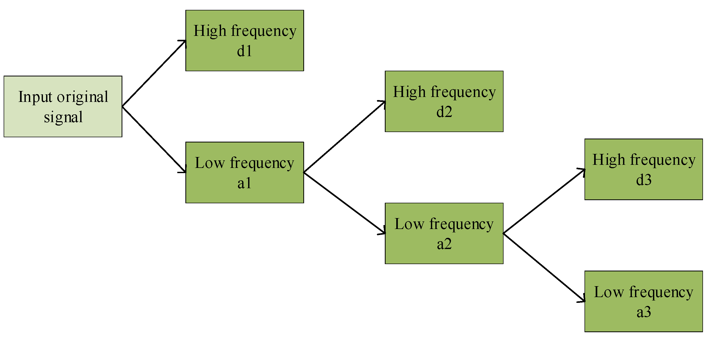
Through the discrete wavelet transform technology, the nonstationary original data is decomposed into several subsequences, and the original data is filtered and denoised.

(c)

An autoencoder is employed to extract highly nonlinear feature data, and then the extracted hidden feature data is input into the BiLSTM framework to predict power generation.

This paper is organized as follows: Section 2 describes some preliminaries. Section 3 illustrates the overall framework of our proposed short-term wind power prediction model based on an autoencoder and BiLSTM. In Section 4, we delineate three case studies, setup the experimental initialization parameters and show the results, and Section 5 presents the conclusions.

2. Preliminaries

2.1. Discrete Wavelet Transform

The wavelet transform has been widely employed in image processing, pattern recognition, signal denoising and other fields [25,26]. It removes noise from the real signal. As one of the main techniques for denoising signals, wavelet transforms greatly improve the accuracy of the time series prediction model. It decomposes the input signal into several low-frequency and high-frequency components. Wavelet transform includes two types: continuous wavelet transform (CWT) and discrete wavelet transform (DWT). The definition of CWT is defined as follows:

$$CW{T}_f(u,s)=<f(t),{\psi }_{u,s}(t)>={\displaystyle {\int }_{-\infty }^{+\infty }f(t)\frac{1}{\sqrt{s}}{\psi }^{*}(\frac{t-u}{s})dt}$$

(1)

where u, s, $f(t)$, $\psi (t)$ and * denote the translation factor, scale factor, real signal, mother wavelet and implies complex conjugate, respectively.

DWT is a Mallat algorithm proposed in 1988. It is widely used in signal decomposition. It reduces the computational complexity and improves the data compression ability, and effectively avoids information redundancy caused by a continuous wavelet transform. The definition of DWT is as follows [27,28]:

$$DWT(j,k)=2^{-\frac{j}{2}}{\displaystyle \sum _{i=0}^{L-1}W(t){\psi }^{*}(\frac{t-k\cdot 2^j}{2^j})}$$

(2)

where j, k, L, $W(t)$ and $\psi (t)$ denote the scale factor, translation factor, length of $W(t)$, input signal and mother wavelet, respectively.

Discrete wavelet decomposition is a multiscale analysis tool that is used to reveal the hidden characteristics of the signal. Due to the nonstationary, fluctuating timing of wind speed, the output power of the wind turbine is unstable. A discrete wavelet transform is used to decompose the original wind speed data into low-frequency components and high-frequency components. The three-level decomposition process using the wavelet transform is shown in Figure 1 [29,30].

2.2. Autoencoder

An autoencoder (AE) consists of an input layer, an encoding layer and a decoding layer. The unsupervised learning method is utilized to extract and represent high-dimensional features of wind power data [31,32,33]. More specifically, AE seeks a set of optimal connection weights by minimizing the reconstruction error between the original input and output. The input vector $X\in R^d$ is input to the hidden layer through the encoder E to generate a potential abstract feature mapping $Z\in R^d$ as in Equation (3) [34,35]. Then, decoder D maps the potential variable Z to the reconstructed output vector $\hat{X}$ as in Equation (4), which is the same size as X.

$$Z=f(W_{1}X+b_1)$$

(3)

$$\hat{X}=\sigma (W_{2}Z+b_2)$$

(4)

where $W_1$ and $W_2$ denote the weight matrices, $f$ and $\sigma$ denote the activation functions and $b_1$ and $b_2$ denote the biases of the encoding layer and the decoding layer.

2.3. Bidirectional LSTM

LSTM is a deep learning architecture for time series prediction that was first proposed by Hochreiter et al. in 1997 [36]. LSTM effectively solves the problem of gradient explosion and vanishing in recurrent neural networks. These networks are good at capturing the dependence between time series data [37,38,39]. However, traditional LSTM can only make use of past context. Graves and Schmidhub proposed a bidirectional LSTM (BiLSTM) to better capture past and future context dependencies [40,41,42]. The bidirectional architecture obtains contextual information from two directions simultaneously, utilizing the forward and backward hidden layers.

In Equation (5), σ denotes the sigmoid function, $\overrightarrow{h_t}$ denotes the outputs of the forward hidden layer, $\overleftarrow{h_t}$ denotes the backward hidden layers. In the function, σ couples the $\overrightarrow{h_t}$ and $\overleftarrow{h_t}$ sequences according to Equation (5). Vector Y = [$y_{t-1},y_t,y_{t+1}$] denotes the output of BiLSTM layer.

$$y_t=\sigma (\overrightarrow{h_t},\overleftarrow{h_t})$$

(5)

3. Algorithm Framework

In this section, our proposed DWT_AE_BiLSTM deep learning algorithm framework is shown in Figure 2, which includes three modules: data processing and denoising module, feature extract module and forecast module. Its implementation details are described as follows:

(a)

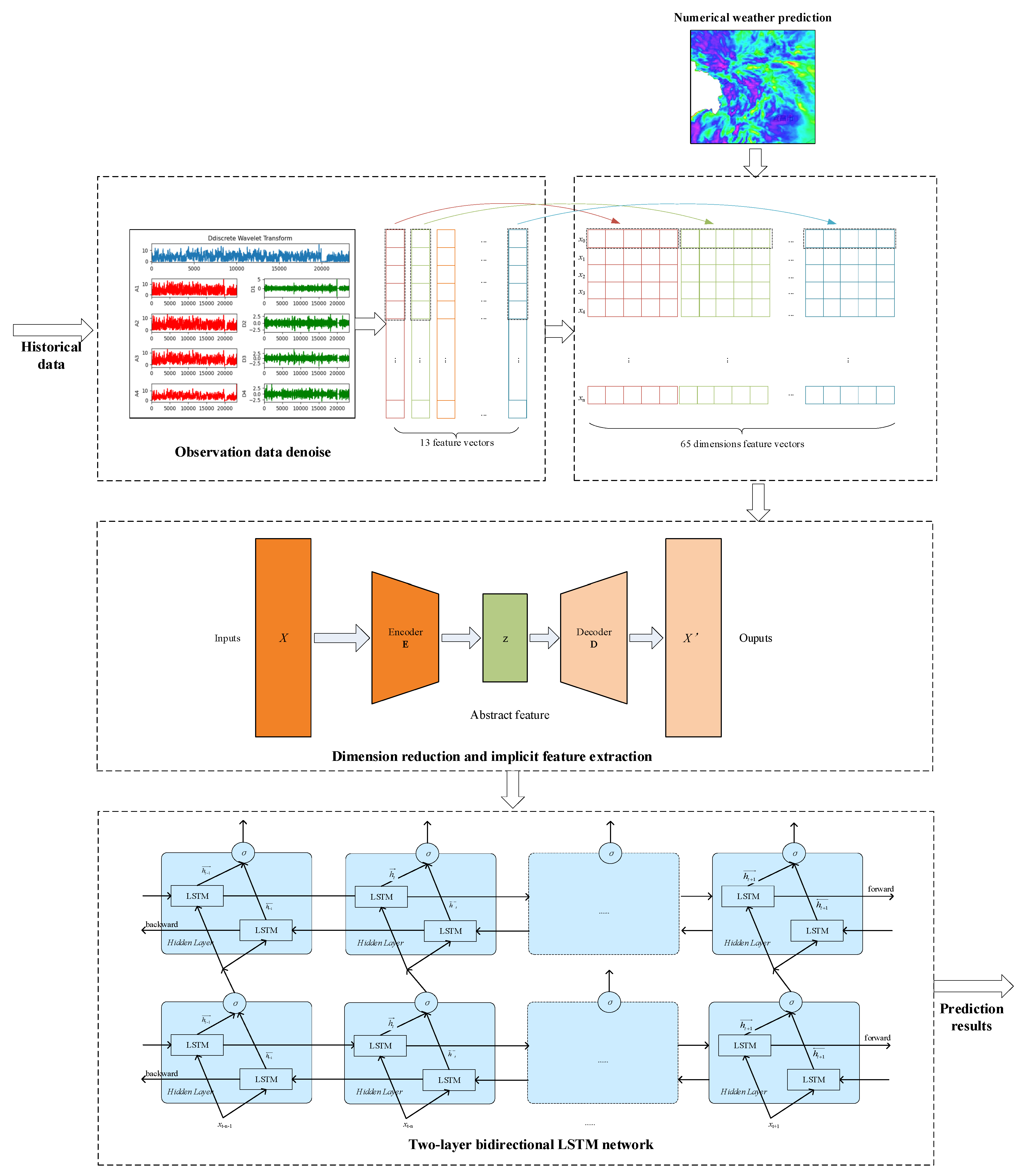
Data processing and denoising module: Firstly, the missing data on a wind farm is interpolated and corrected. Then, the discrete wavelet transform technology is used to decompose the nonstationary wind power time series data into low-frequency component and high-frequency component. These components exhibit a greater degree of stationarity and may be forecasted more easily. Input data mainly includes wind tower observation data, wind farm total active power and numerical weather prediction (NWP) data. Wind tower observation data and NWP data include 12 meteorological elements, i.e., wind speed and direction at heights of 10 m, 30 m, 50 m and 70 m, and turbine hub, temperature, humidity and pressure. All of the data time resolutions are 15 min.

(b)

Feature extract module: Based on step (a), in addition to the actual power of the power station, there are 13 elements in total. Each element takes five elements in chronological order to form a 65-dimensional vector, which is input into the autoencoder. The features are compressed into a 30-dimensional vector through the training of the autoencoder.

(c)

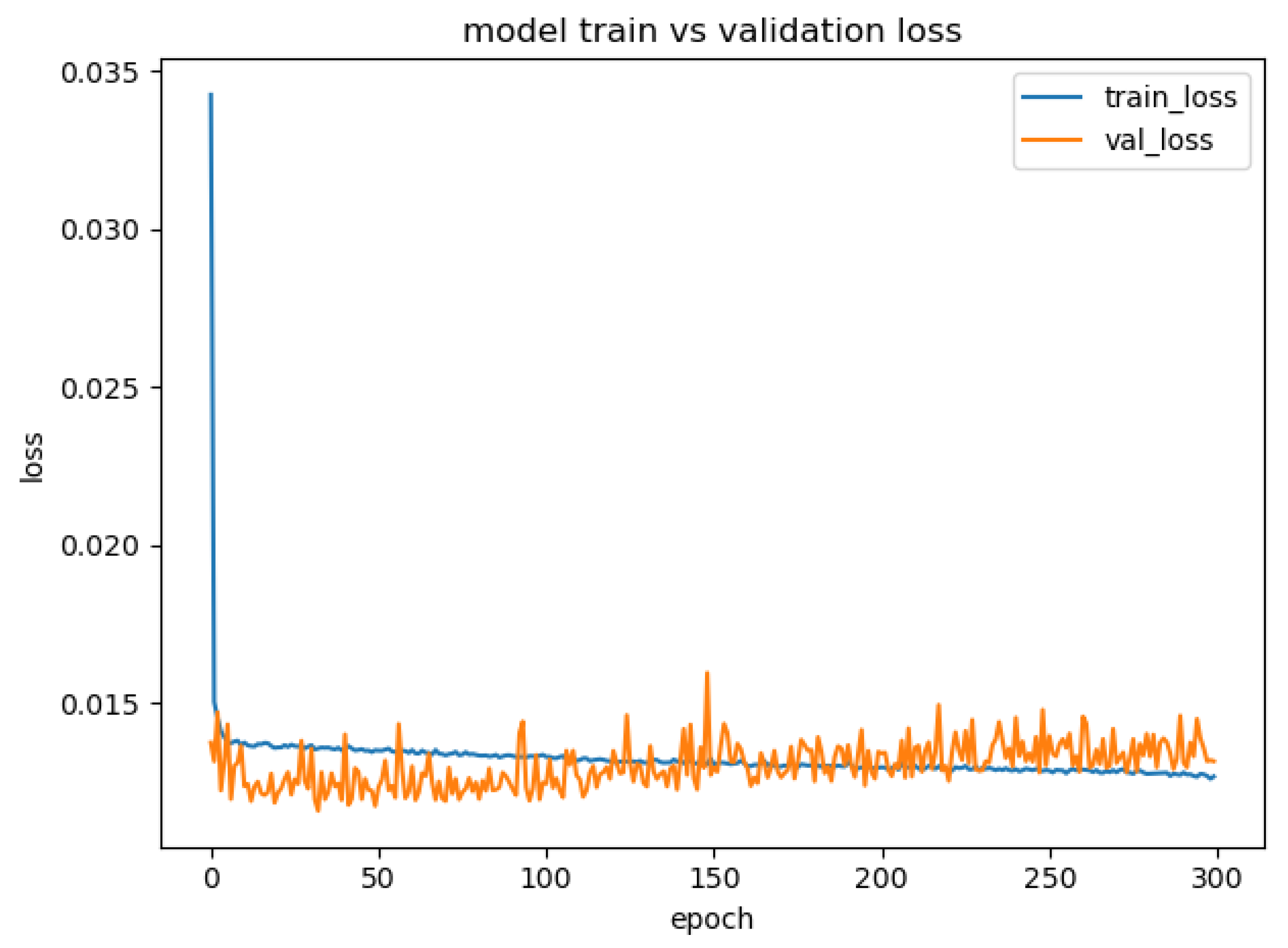
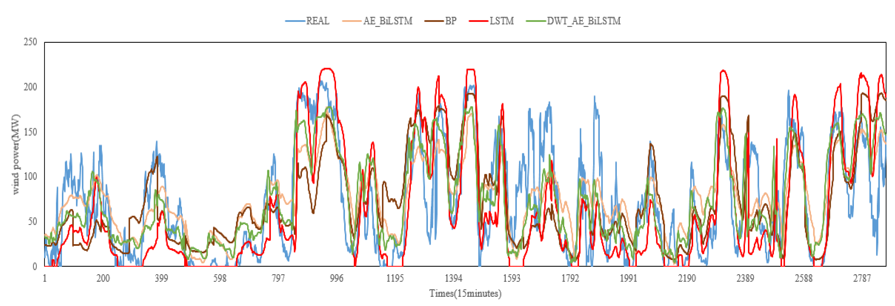
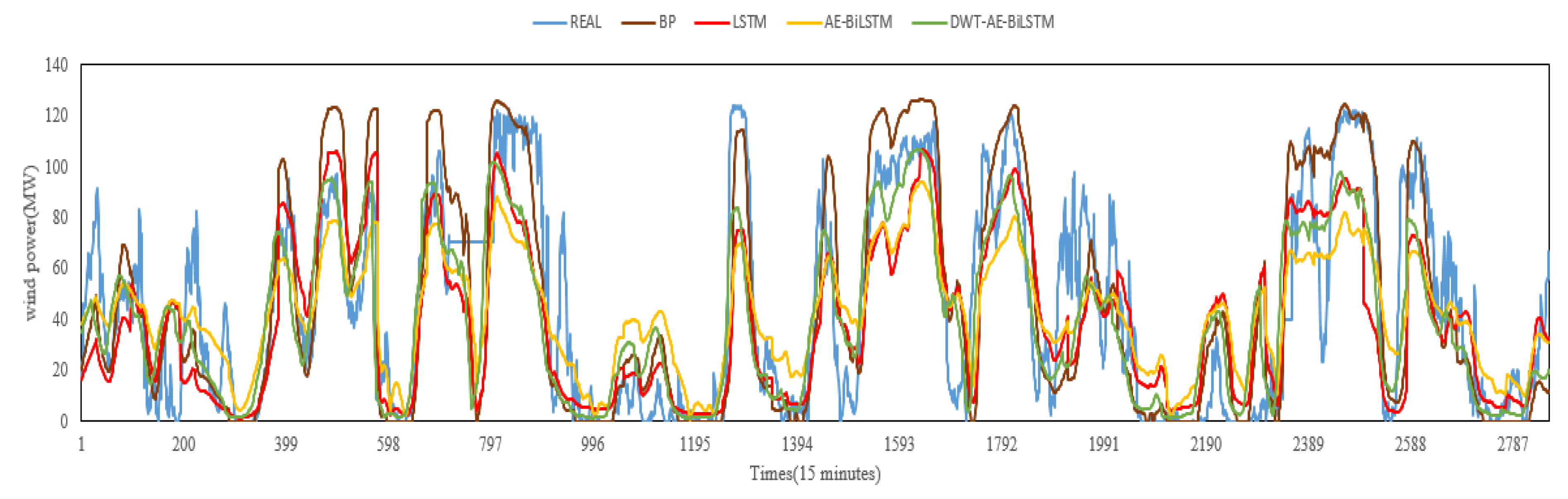
Forecast module: The compressed features in step (b) are input into the bidirectional LSTM to predict the short-term power generation of the wind farm combined with NWP. Bidirectional, two-layer stacked LSTMs are used. We apply the Adam optimization method for training. The grid search method is used to determine the hyper-parameters, and the optimal configuration of model parameters is obtained from the validation set. The final optimal parameters learn rate = 1 × 10⁻³ and batch size = 128. The dataset utilized in this study comprises data from the calendar year 2018, which has been divided into training and validation sets consisting of 70% and 30% of the data, respectively. In order to evaluate the predictive performance of the model, data from four representative months of the year 2019 were handpicked for comparison against the forecasted outcomes. The results are illustrated in Figure 3, which displays the respective losses of the training and validation sets for Wind Farm #1.

4. Experimental Design

The whole power forecast framework was completed in Python 3.7. We implemented our DWT_AE_BiLSTM framework based on a deep learning platform with Tensorflow version 1.13. All models were built using Keras 2.1.3. The models run on a Windows 7 operating system, Intel (R) Core (TM) i7-2600 CPU@3.40 GHz and 8 GB RAM.

4.1. Data Description

In order to make the experiment more representative, four typical months of a year were selected for each wind farm, namely the real-time wind farm power output data, wind tower measurements and numerical weather forecast. The time interval between two adjacent data points is 15 min. The unit for the wind power data is MW. The three wind farms are located in Suizhou (Wind Farm #1, installed capacity is 110 MW), Huanggang (Wind Farm #2, installed capacity is 220 MW), and Lichuan (Wind Farm #4, installed capacity is 126.3 MW). These wind farms are located in Hubei Province, which has different altitudes and topographical features.

4.2. Performance Evaluation Metrics

In this paper, we use four evaluation indicators to evaluate the performance of the forecasting model. The matrices are normalized root mean square error (PA), mean absolute error (MAE) and mean absolute percentage error (MAPE). These matrices are widely used to evaluate the performance of wind power forecasting models [43,44,45]. Prediction accuracy (PA) and the performance evaluation metrics are calculated by (6)–(9), respectively.

$$NRMSE=\frac{1}{Cap}\sqrt{\frac{1}{N}{\displaystyle \sum _{}^{}{(P_f^i-P_o^i)}^2}}$$

(6)

$$MAE=\frac{{\displaystyle \sum _{i=1}^N\left|P_f^i-P_o^i\right|}}{N}$$

(7)

$$MAPE=\frac{{\displaystyle \sum _{i=1}^N\left|P_f^i-P_o^i\right|}}{N}/Cap\times 100\%$$

(8)

$$PA=(1-NRMSE)\times 100\%$$

(9)

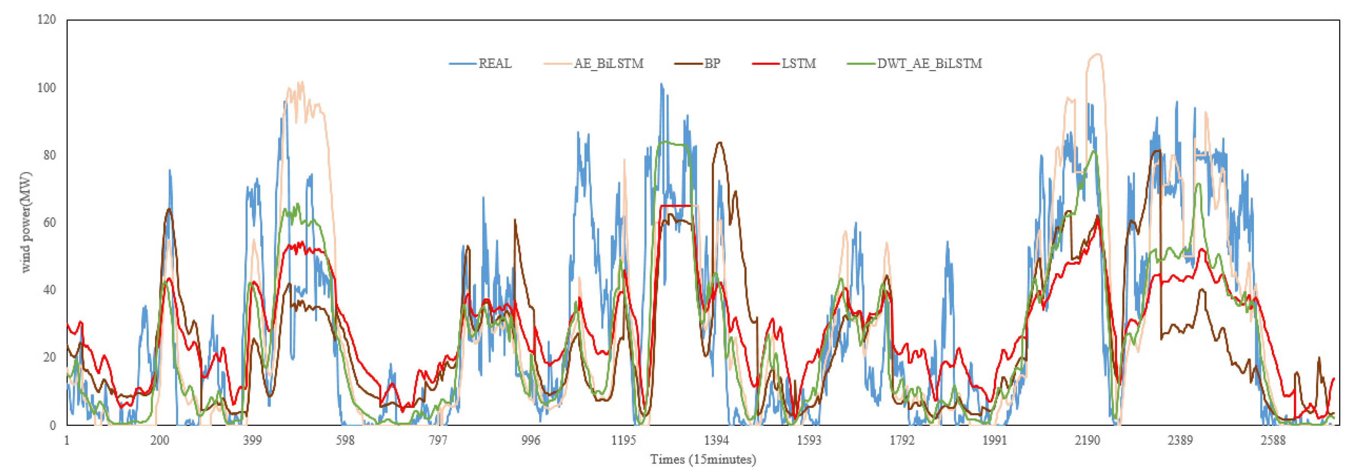
4.3. Results and Analysis

To verify the performance of the proposed model, the experiment was carried out on three wind farms. To validate the efficiency of the proposed model, we compared the DWT_AE_BiLSTM model with three models: autoencoder and bidirectional long short-term memory without DWT (AE_BiLSTM), long short-term memory (LSTM) and traditional back propagation (BP).

Table 1. Performance evaluation of each prediction algorithm in Wind Farm #1.

Month	Algorithms	PA (%)	MAE (MW)	MAPE (%)
1	DWT_AE_BiLSTM	84.69	12.03	10.94
	AE_BiLSTM	83.40	13.10	11.91
	LSTM	82.08	14.25	12.95
	BP	78.24	17.48	15.89
4	DWT_AE_BiLSTM	82.36	13.58	12.35
	AE_BiLSTM	81.33	15.73	14.30
	LSTM	79.04	16.33	14.85
	BP	78.77	16.93	15.39
7	DWT_AE_BiLSTM	83.63	11.65	12.41
	AE_BiLSTM	82.68	12.39	11.26
	LSTM	82.10	12.57	11.43
	BP	81.93	12.60	11.45
10	DWT_AE_BiLSTM	90.69	6.34	5.76
	AE_BiLSTM	89.76	7.14	6.49
	LSTM	88.30	9.05	8.23
	BP	86.99	10.02	9.11

presents the forecast performance of each model in Wind Farm #1. The DWT_AE_BiLSTM model demonstrates the highest prediction accuracy (PA) across all the months, with an increase of 6.45% compared with the BP algorithm in February and reaching a maximum of 90.69% in all months by October. DWT_AE_BiLSTM model is 6.45%, 3.59%, 1.7% and 3.7% higher than the BP algorithm in January, April, July and October, respectively, with an average increase of 3.86%, while MAE was decreased by 4.41 MW, 3.79 MW, 4.88 MW and 6.62 MW, respectively. The BP model forecast exhibits lower accuracy in the time periods 2352–2535 and 1259–1342, while it shows significantly greater accuracy in the time periods 961–1002 and 1387–1482, as depicted in Figure 4.

Table 2. Performance evaluation of each prediction algorithm in Wind Farm #2.

Month	Algorithms	PA(%)	MAE(MW)	MAPE(%)
1	DWT_AE_BiLSTM	84.75	29.27	13.30
	AE_BiLSTM	81.42	30.41	13.82
	LSTM	80.30	31.51	14.32
	BP	79.45	33.19	15.09
4	DWT_AE_BiLSTM	82.65	30.31	13.78
	AE_BiLSTM	81.71	33.94	15.43
	LSTM	80.45	34.23	15.56
	BP	80.35	34.47	15.67
7	DWT_AE_BiLSTM	84.11	28.17	12.80
	AE_BiLSTM	83.65	29.36	13.35
	LSTM	83.23	30.38	13.81
	BP	82.95	32.42	14.74
10	DWT_AE_BiLSTM	84.35	28.18	12.81
	AE_BiLSTM	81.57	29.49	13.40
	LSTM	81.31	32.07	14.58
	BP	80.25	34.94	15.88

illustrates the comparison of the prediction performance of each model in Wind Farm #2. The DWT_AE_BiLSTM model shows the highest PA in January (84.75%) and the lowest in April (82.65%). In April, the BP and LSTM forecast accuracies are similar, while the PA of BiLSTM is 1.26% higher than LSTM, and DWT_AE_BiLSTM is 0.94% higher than AE_BiLSTM, as indicated in Figure 5. In all months, DWT_AE_BiLSTM model is 5.3%, 2.3%, 1.16% and 4.1% higher than the BP algorithm in January, April, July and October, respectively, and 3.22% higher on average in 4 months.

Figure 6 shows that in the April forecast for Wind Farm #3, the proposed model DWT_AE_BiLSTM is 2.58%, 2.67%, 3.55% and 4.93% higher than the BP algorithm in January, April, July and October, respectively, and 3.42% higher on average in 4 months. The BP prediction model is significantly higher than the real result in the 471–511, 559–563 and 1538–1662 time periods, the PA of BiLSTM is 0.49% higher than that of LSTM, which also proves that the prediction accuracy can be improved by using an autoencoder feature extraction. After using DWT to denoise, the prediction accuracy was further improved.

In addition, Table 1, Table 2 and

Table 3. Performance evaluation of each prediction algorithm in Wind Farm #3.

Month	Algorithms	PA(%)	MAE(MW)	MAPE(%)
1	DWT_AE_BiLSTM	82.23	15.17	12.01
	AE_BiLSTM	81.47	15.53	12.30
	LSTM	81.02	18.81	14.89
	BP	79.65	19.58	15.50
4	DWT_AE_BiLSTM	82.12	16.86	13.35
	AE_BiLSTM	81.59	17.10	13.54
	LSTM	81.10	19.38	15.34
	BP	79.42	20.65	16.35
7	DWT_AE_BiLSTM	82.00	16.37	12.96
	AE_BiLSTM	81.48	17.30	13.70
	LSTM	79.47	18.91	14.97
	BP	78.45	21.25	16.83
10	DWT_AE_BiLSTM	88.66	8.27	6.55
	AE_BiLSTM	87.65	10.07	7.97
	LSTM	84.12	14.03	11.11
	BP	83.73	14.89	11.79

and Figure 4, Figure 5 and Figure 6 depict the performance of each model on all evaluation metrics in detail. Among all the models, the DWT_AE_BiLSTM model had the best prediction accuracy in terms of PA, MAE and MAPE. The BP model had the lowest prediction accuracy of all performance indexes. Obviously, through the comparative analysis of the short-term predictions of three wind farms, the prediction algorithm based on the deep learning frameworks LSTM, AE_LSTM, and DWT_AE_BiLSTM had a better prediction effect than the traditional neural network prediction algorithm BP.

In summary, it is clearly seen that the proposed model DWT_AE_BiLSTM shows the best prediction ability in three different wind farms. The performance of the BP prediction algorithm is extremely unstable; it oscillates up and down, and the prediction is either too large or too small. The proposed prediction algorithm shows better prediction performance than other algorithms. All deep learning models have better prediction performance than traditional neural networks. The prediction model using LSTM and an autoencoder for feature extraction is better than the LSTM model. Bidirectional LSTM is better than LSTM. Experiments show that a discrete wavelet transform can effectively remove the nonstationary noise data in wind power prediction, and an autoencoder can capture more abstract and hidden nonlinear features. The proposed DWT_AE_BiLSTM algorithm model has good universality and generalization ability in all situations.

5. Conclusions

This paper proposes a wind power forecast model that consists of a data processing and denoising module, a feature extract module and a bidirectional deep learning forecast module. The experiment is carried out on datasets collected from three different wind farms in Hubei Province. Compared with the BP model, the proposed model has increased by 3.86%, 3.22% and 3.42% in three wind farms, respectively. The comparison results show that: (a) by using a sparse autoencoder, the dimension of the original data is reduced, and it discovers more abstract hidden features; (b) all performance indexes of the proposed model outperform other machine learning models; and (c) the proposed model shows robustness and reliability in three wind farms.

References

1. GWEC. Global Wind Report 2021; Global Wind Energy Council: Brussels, Belgium, 2021. [Google Scholar]
2. Yuan, X.H.; Chen, C.; Yuan, Y.B.; Huang, Y.H.; Tan, Q.X. Short-term wind power prediction based on LSSVMGSA model. Energy Convers. Manag. 2015, 101, 393–401. [Google Scholar] [CrossRef]
3. Kim, H.; Powell, W. Optimal energy commitments with storage and inter-mittent supply. Oper. Res. 2011, 59, 1347–1360. [Google Scholar] [CrossRef] [Green Version]
4. Munoz, C.; Marquez, F.; Lev, B.; Arcos, A. New pipe notch detection and location method for short distances employing ultrasonic guided waves. Acta Acust. United Acust. 2017, 103, 772–781. [Google Scholar] [CrossRef] [Green Version]
5. Giebel, G.; Brownsword, R.; Kariniotakis, G.; Denhard, M.; Draxl, C. The State-of-the-Art in Short-Term Prediction of Wind Power: A Literature Overview. 2011. Available online: https://academic.microsoft.com/paper/2593375484 (accessed on 16 January 2023).
6. Carpinone, A.; Giorgio, M.; Langella, R.; Testa, A. Markov chain modeling for very-short-term wind power forecasting. Electr. Power Syst. Res. 2015, 122, 152–158. [Google Scholar] [CrossRef] [Green Version]
7. Monforti, F.; Gonzalez-Aparicio, I. Comparing the impact of uncertainties on technical and meteorological parameters in wind power time series modelling in the european union. Appl. Energy 2017, 206, 439–450. [Google Scholar] [CrossRef]
8. Wang, K.; Qi, X.; Liu, H.; Song, J. Deep belief network based k-means cluster approach for short-term wind power forecasting. Energy 2018, 165, 840–852. [Google Scholar] [CrossRef]
9. Lange, M.; Focken, U. Physical Approach to Short-Term Wind Power Prediction; Springer: Berlin/Heidelberg, Germany, 2006. [Google Scholar]
10. Liu, Y.; Shi, J.; Yang, Y.; Han, S. Piecewise support vector machine model for short-term wind-power prediction. Int. J. Green Energy 2009, 6, 479–489. [Google Scholar] [CrossRef]
11. Min, D.; Hao, Z.; Hua, X.; Min, W.; Kang-ZLiuc Yosuke, N. A time series model based on hybrid-kernel least-squares support vector machine for short-term wind power forecasting. ISA Trans. 2021, 108, 58–68. [Google Scholar]
12. Yang, L.; He, M.; Zhang, J.; Vittal, V. Support-vector-machine-enhanced markov model for short-term wind power forecast. IEEE Trans. Sustain. Energy 2015, 6, 791–799. [Google Scholar] [CrossRef]
13. Lahouar, A.; Slama, J.B.H. Hour-ahead wind power forecast based on random forests. Renew. Energy 2017, 109, 529–541. [Google Scholar] [CrossRef]
14. Wan, J.; Liu, J.; Ren, G.; Guo, Y.; Yu, D.; Hu, Q. Day-ahead prediction of wind speed with deep feature learning. Int. J. Pattern. Recogn. Artif. Intellig. 2016, 30, 1650011. [Google Scholar] [CrossRef]
15. Wang, H.; Wang, G.; Li, G.; Peng, J.; Liu, Y. Deep belief network based deterministic and probabilistic wind speed forecasting approach. Appl. Energy 2016, 182, 80–93. [Google Scholar] [CrossRef]
16. Yu, W.; Mechefske, C.; Kim, Y. Time Series Reconstruction Using a Bidirectional Recurrent Neural Network based Encoder-Decoder Scheme. In AIAC18: 18th Australian International Aerospace Congress (2019): HUMS—11th Defence Science and Technology (DST) International Conference on Health and Usage Monitoring (HUMS 2019): ISSFD—27th International Symposium on Space Flight Dynamics (ISSFD); Engineers Australia, Royal Aeronautical Society: Melbourne, Australia, 2019; pp. 876–884. Available online: https://search.informit.com.au/documentSummary;dn=324293936594299;res=IELENG (accessed on 15 February 2023).
17. Liu, X.; Zhou, J.; Qian, H. Short-term wind power forecasting by stacked recurrent neural networks with parametric sine activation function. Electr. Power Syst. Res. 2021, 192, 107011. [Google Scholar] [CrossRef]
18. Higashiyama, K.; Fujimoto, Y.; Hayashi, Y. Feature extraction of nwp data for wind power forecasting using 3d-convolutional neural networks. Energy Procedia 2018, 155, 350–358. [Google Scholar] [CrossRef]
19. Qu, X.; Kang, X.; Zhang, C.; Jiang, S.; Ma, X. Short-term prediction of wind power based on deep long short-term memory. In Proceedings of the 2016 IEEE PES Asia-Pacific Power and Energy Engineering Conference (APPEEC), Xi’an, China, 25–28 October 2016; pp. 1148–1152. [Google Scholar]
20. Liu, Y.; Liu, L. Wind power prediction based on LSTM-CNN optimization. Sci. J. Intell. Syst. Res. 2021, 277, 285. [Google Scholar]
21. Yin, H.; Ou, Z.; Chen, D.; Meng, A. Ultra-short-term wind power prediction based on quadratic mode decomposition and cascaded deep learning. Power Syst. Technol. 2020, 44, 445–453. [Google Scholar]
22. Lawal, A.; Rehman, S.; Alhems, L.M.; Alam, M.M. Wind speed prediction using hybrid 1d-CNN and BLSTM network. IEEE Access 2021, 9, 156672–156679. [Google Scholar] [CrossRef]
23. Wang, C.; Zhang, H.; Ma, P. Wind power forecasting based on singular spectrum analysis and a new hybrid laguerre neural network. Appl. Energy 2020, 259, 114139. [Google Scholar] [CrossRef]
24. Viet, D.; Phuong, V.; Duong, M.; Tran, Q. Models for short-term wind power forecasting based on improved artificial neural network using particle swarm optimization and genetic algorithms. Energies 2020, 13, 2873. [Google Scholar] [CrossRef]
25. Shi, Z.; Liang, H.; Dinavahi, V. Direct interval forecast of uncertain wind power based on recurrent neural networks. IEEE Trans. Sustain. Energy 2018, 9, 1177–1187. [Google Scholar] [CrossRef]
26. Dautov, Ç.P.; Özerdem, M.S. Introduction to Wavelets and their applications in signal denoising. Bitlis Eren Univ. J. Sci. Technol. 2018, 8, 1–10. [Google Scholar] [CrossRef] [Green Version]
27. Daubechies, I. Ten Lectures on Wavelets; SIAM: Philadelphia, PA, USA, 1992. [Google Scholar]
28. Montanari, L.; Basu, B.; Spagnoli, A.; Broderick, B. A padding method to reduce edge effects for enhanced damage identification using wavelet analysis. Mech. Syst. Signal Process. 2015, 52–53, 264–277. [Google Scholar] [CrossRef]
29. Hu, J.M.; Wang, J.Z. Short-term wind speed prediction using empirical wavelet transform and Gaussian process regression. Energy 2015, 93, 1456–1466. [Google Scholar] [CrossRef]
30. Gong, Z.Q.; Zou, M.W.; Gao, X.Q.; Dong, W.J. On the difference between empirical mode decomposition and wavelet decomposition in the nonlinear time series. Acta Phys. Sin. 2005, 54, 3947–3957. [Google Scholar] [CrossRef]
31. Li, S.; He, H.; Li, J. Big data driven lithium-ion battery modeling method based on SDAE-ELM algorithm and data pre-processing technology. Appl. Energy 2019, 242, 1259–1273. [Google Scholar] [CrossRef]
32. Chen, Y.; Lin, Z.; Zhao, X.; Wang, G.; Gu, Y. Deep learning-based classification of hyperspectral data. IEEE J. Sel. Top. Appl. Earth Observ. Remote Sens. 2014, 7, 2094–2107. [Google Scholar] [CrossRef]
33. Gensler, A.; Henze, J.; Sick, B.; Raabe, N. Deep learning for solar power forecasting—An approach using AutoEncoder and LSTM Neural Networks. In Proceedings of the 2016 IEEE International Conference on Systems, Man, and Cybernetics (SMC), Budapest, Hungary, 9–12 October 2016; pp. 2858–2865. [Google Scholar]
34. Cheng, F.; He, Q.; Zhao, J. A novel process monitoring approach based on variational recurrent autoencoder. Comput. Chem. Eng. 2019, 129, 106515. [Google Scholar] [CrossRef]
35. Klampanos, I.; Davvetas, A.; Andronopoulos, S.; Pappas, C.; Ikonomopoulos, A.; Karkaletsis, V. Autoencoder-driven weather clustering for source estimation during nuclear events. Environ. Model. Software 2018, 102, 84–93. [Google Scholar] [CrossRef] [Green Version]
36. Hochreiter, S.; Schmidhuber, J. Long short-term memory. Neural Comput. 1997, 9, 1735–1780. [Google Scholar] [CrossRef]
37. Goodfellow, I.; Bengio, Y.; Courville, A. Deep Learning; The MIT Press: Cambridge, MA, USA, 2016; p. 800. ISBN 978-0-262-03561-3. Available online: http://www.deeplearningbook.org (accessed on 15 February 2023).
38. Mesnil, G.; He, X.; Deng, L.; Bengio, Y. Investigation of recurrent-neural-network architectures and learning methods for spoken language understanding. In Proceedings of the 14th Annual Conference of the International Speech Communication Association, Lyon, France, 25–29 August 2013; pp. 1–5. [Google Scholar]
39. Pascanu, R.; Gulcehre, C.; Cho, K.; Bengio, Y. How to construct deep recurrent neural networks. arXiv 2013, arXiv:1312.6026. [Google Scholar]
40. Zhang, J.; Yan, J.; Infield, D.; Liu, Y.; Lien, F.-S. Short-term forecasting and uncertainty analysis of wind turbine power based on long short-term memory network and gaussian mixture model. Appl. Energy 2019, 241, 229–244. [Google Scholar] [CrossRef] [Green Version]
41. Graves, A.; Schmidhuber, J. Framewise phoneme classification with bidirectional Lstm and other neural network architectures. Neural Netw. 2005, 18, 602–610. [Google Scholar] [CrossRef] [PubMed]
42. Schuster, M.; Paliwal, K.K. Bidirectional recurrent neural networks. IEEE Trans. Signal Process. 1997, 45, 2673–2681. [Google Scholar] [CrossRef] [Green Version]
43. Wang, J.; Niu, T.; Lu, H.; Yang, W.; Du, P. A Novel Framework of Reservoir Computing for Deterministic and Probabilistic Wind Power Forecasting. IEEE Trans. Sustain. Energy 2019, 11, 337–349. [Google Scholar] [CrossRef]
44. Lin, Y.; Yang, M.; Wan, C.; Wang, J.; Song, Y. A multi-model combination approach for probabilistic wind power forecasting. IEEE Trans. Sustain. Energy 2019, 10, 226–237. [Google Scholar] [CrossRef] [Green Version]
45. Zhao, Y.; Ye, L.; Pinson, P.; Tang, Y.; Lu, P. Correlation-constrained and sparsity-controlled vector autoregressive model for spatio-temporal wind power forecasting. IEEE Trans. Power Syst. 2018, 33, 5029–5040. [Google Scholar] [CrossRef] [Green Version]
Figure 1. The schematic diagram of discrete wavelet transform decomposition.
Applsci 13 04042 g001
Figure 2. Proposed flowchart of DWT_AE_BiLSTM deep learning algorithm framework. Numerical weather prediction (NWP) and historical observation data are used as input data, discrete wavelet transform (DWT) is used to denoise the data, autoencoder (AE) is used for feature extraction and Bi-LSTM is used for prediction.
Applsci 13 04042 g002
Figure 3. The loss of the validation set and the training set of Wind Farm #1.
Applsci 13 04042 g003
Figure 4. Comparison among different wind power short-term prediction models of Wind Farm #1 in April 2019.
Applsci 13 04042 g004
Figure 5. Comparison among different wind power short-term prediction models of Wind Farm #2 in April 2019.
Applsci 13 04042 g005
Figure 6. Comparison among different wind power short-term prediction models of Wind Farm #3 in April 2019.
Applsci 13 04042 g006