Moment-Based Stochastic Analysis of a Bistable Energy Harvester with Matching Network

Abstract

We discuss the analysis of a piezoelectric energy harvester for random mechanical vibrations, and we assess the performance improvement guaranteed by interposing a matching network between the transducer and the electrical load, in terms of average output power and power efficiency. The mathematical model describing the harvester is a system of stochastic differential equations, where both cases of linear and nonlinear devices are considered. In the linear case, the power delivered to the load is increased by a factor of about 20 with respect to the direct connection, with a similar increase in the conversion efficiency. In the nonlinear case, we use a moment closure technique to calculate the first- and second-order moments of the electro-mechanical variables in the weak noise limit. Moment calculation is used to determine the optimal values of the matching network components that maximize the performance. In the strong noise limit, the state equations are integrated numerically to determine the same performance metrics. Our analysis shows that a properly designed matching network improves the performance by a significant amount, especially at low noise intensity.

1. Introduction

Scavenging ambient dispersed energy available for conversion to electrical power represents the ultimate solution for self-powering individual nodes of wireless sensor networks [1,2,3,4] and, more in general, internet of things (IoT) wireless interconnected devices.

Although the possible energy sources are quite varied, ranging from human motion to thermal gradients and high-frequency electromagnetic radiation [5,6,7,8], ambient parasitic vibrations are particularly promising due to several characteristics, such as their significant power availability, the ease of conversion into an electrical form making use of a certain number of transducers, and, last but not least, the fact that they are ubiquitous [9,10,11,12,13].

The modeling, and thus also the design, of vibration energy harvesters requires in the first place to properly describe the energy source, i.e., the mechanical vibrations available for energy collection. Some considerations on the harvester design can be carried out based on a simplified description, in which vibrations are assumed purely sinusoidal [14,15,16,17,18,19,20,21]. In other words, this amounts to assume that the energy is concentrated at a single frequency value or, mathematically speaking, the power spectrum is a delta function vs. frequency. On the other hand, a more physical description should take into account the spread of the vibration energy over a continuous frequency range. For this task, the more obvious approach amounts to a random description of vibrations [22,23,24,25,26,27,28,29].

From the designer point of view, a stochastic description of external sources poses major challenges, especially when nonlinear effects are taken into account, as the application of the combined machinery of stochastic analysis [30,31] and nonlinear dynamics [32] is required.

A second major challenge is represented by the obvious requirement to design harvesting systems with a very high efficiency. In fact, energy harvesters (or, more in general, electrical power supplies), are often working far from their optimal condition due to a non-ideal energy transfer from the (mechanical) source to the (electrical) load. Such an operating condition can be conveniently represented exploiting an electro-mechanical analogy, allowing for the construction of an equivalent circuit describing the entire harvester [28,33]: this representation, in turn, suggests the introduction of a matching network between the harvesting device and the electrical load to eliminate, or at least mitigate, the mismatch [18,19,34]. Impedance matching is a classical design technique that has been exploited in RF and microwave electronics for about 70 years [35,36,37]; however, in other electronics areas, the energy transfer improvement is mostly limited to power factor correction schemes.

A solution inspired by power factor correction is the connection of a shunted reactive element (capacitor or inductor) in parallel to the resistive load [18,34,38,39]. The role of the shunted element is to reduce the time lag between the voltage and current in the load, thus reducing the amount of power reflected from the load to the source. An alternative solution, based on impedance matching theory, consists in interposing a matching network between the harvester and the electrical load. The matching network must be designed to eliminate the impedance mismatch between the mechanical and the electrical parts. The advantage offered by the matching network solution is that it not only reduces the power reflected from the load to the source but also maximizes the average power absorbed by the load, in general outperforming power factor corrected solutions. Obviously, perfect matching is achievable only at a specific frequency. Still, the matching network can be optimized to offer partial matching over a relatively wide frequency interval, maximizing the average power absorbed by the load and the power conversion efficiency, even for multi-frequency or broadband inputs.

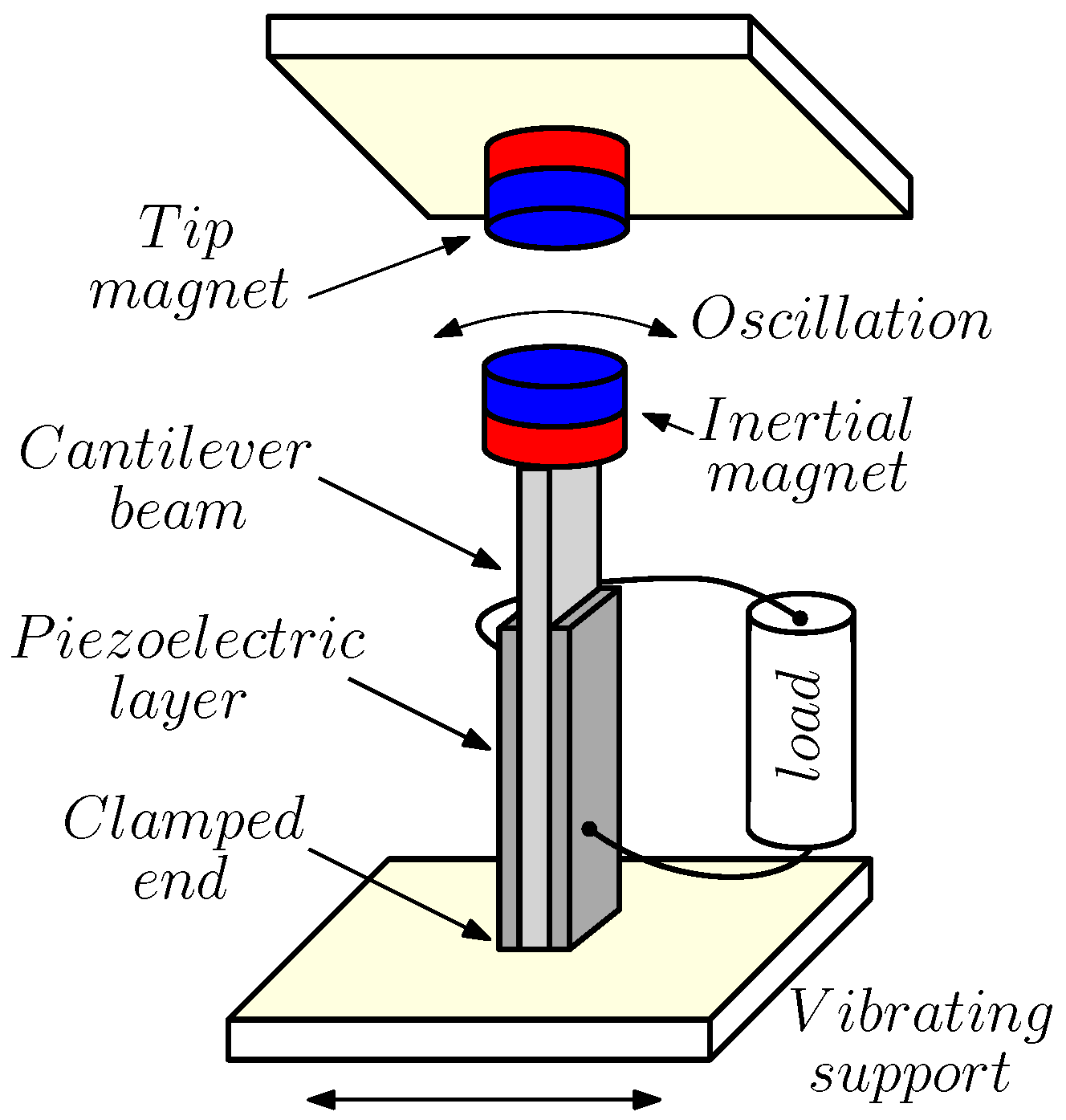
In this work, we study a bistable piezoelectric energy harvester, as schematized in Figure 1, subject to random mechanical vibrations. In this device, a cantilever beam is fixed at one end to a vibrating support, with a magnet of mass m at the opposite end to amplify oscillations. Vibrations of the support induce oscillations of the beam that in turn are transformed into electrical power by means of layers of a piezoelectric material deposed on the cantilever. Nonlinearity is introduced in the design by the tip magnet, that is fixed to a support in front of the inertial magnet but with opposed polarities, to create a biased inverted pendulum with magnetic repulsive force. When the two magnets are close enough, magnetic repulsion forces the beam to the left or to the right of the vertical position. The unforced system exhibits bi-stability, with two stable equilibrium points, each with its own basin of attraction, separated by an unstable saddle, corresponding to the vertical position.

We show novel results derived through stochastic analysis complemented by numerical approaches. The energy harvester description derives from modeling the mechanical part, the linear piezoelectric materials, and the circuit representation of the electrical load. Nonlinearities are included by means of a proper model for the mechanical elastic potential. The result is a description in the form of a stochastic differential equation (SDE) system.

For the linear energy harvester, we use stochastic calculus to analytically evaluate the output average power and the power efficiency. For the nonlinear system, the same quantities cannot be computed analytically, because the resulting stochastic differential equations are nonlinear and cannot be solved. To overcome this issue, we resort to a moment closure technique that permits to calculate the moments of the probability distribution for the electro-mechanical variables in the weak noise limit. In the medium-strong noise regime, we use stochastic numerical integration schemes to calculate the output average power and power efficiency.

Inspired by our recent work on the application of circuit theory to improve the efficiency of energy harvesting systems, we interpose an $LC$ matching network between the transducer and the load [18,19], whose advantages are assessed in terms of the output (i.e., on the load) average voltage, output average power and conversion power efficiency.

The paper is organized as follows: In Section 2, we derive the stochastic differential equations that describe the energy harvester subject to random vibrations, modeled as a white Gaussian noise. As a first contribution, in Section 3, we derive the equation governing the power balance of the electro-mechanical system, showing that determination of the output average power and of the power efficiency requires to calculate the variance of the output voltage. Section 4 is dedicated to the second main contribution: we introduce a novel, systematic procedure to derive dimensionless stochastic differential equations describing the system. In particular, we show how dimensionless time must be introduced to correctly take into account the stochastic nature of the governing equations. Section 5 is devoted to the analysis of a linear energy harvester, showing how stochastic calculus can be used for the design and optimization of the matching network.

Section 6 represents the main contribution of the work: we develop a methodology based on the Gaussian moment closure technique for the design and optimization of the matching network for nonlinear energy harvesters, a quite important result, as few techniques exist for the design of nonlinear systems. We show that the optimized matching network increases the average harvested power and power conversion efficiency by more than 30 times in the weak noise limit, and by more than 5 times for medium-strong noise intensity. Finally, Section 7 is devoted to conclusions.

2. Stochastic Differential Equations and Energy Harvesting System Modeling

Mechanical vibrations are random in nature, and thus they are best described as a stochastic process.

Let $(\mathsf{\Omega },\mathcal{F},P)$ be a probability space, where $\mathsf{\Omega }$ is the sample space, $\mathcal{F}={\left({\mathcal{F}}_t\right)}_{t\ge 0}$ is a filtration, i.e., the $\sigma$-algebra of all the events, and P a probability measure. A vector-valued stochastic process ${\mathbf{X}}_t$ is a vector of random variables parameterized by $t\in T$. We adopt the standard notation used in probability: capital letters denote random variables, while lower case letters denote their possible values. The parameter space T is usually the half-line $[0,+\infty ]$. Alternatively, the stochastic process can be thought of as the function ${\mathbf{X}}_t:\mathsf{\Omega }\times T\mapsto {\mathbb{R}}^d$.

The energy of mechanical vibrations is typically concentrated at low frequencies, but if the frequency spectrum is wide enough, and the noise correlation time is negligible, a white Gaussian noise process may represent a reasonable approximation. A truly white noise process cannot exist in the real world, as the flat spectrum characteristic of a white process implies an infinite power. Even if the white source overestimates the available power, a finite bandwidth is usually recovered since the deterministic dynamics normally embeds a low-pass behavior. Therefore, the white process approximation is quite common in the literature, and a well-developed theory is available, making the white noise approximation very convenient from the mathematical point of view [22,23,25,30,31,39,40,41,42,43].

White Gaussian noise is the “formal” derivative of a Wiener process. A one-dimensional Wiener process $W_t=W\left(t\right)$ is characterized by $\mathrm{E}\left[W_t\right]=0$ (symbol $\mathrm{E}\left[X_t\right]$ denotes expectation of the stochastic process $X_t$ with respect to the measure P), covariance $\mathrm{cov}(W_t,W_s)=\mathrm{E}\left[W_t{W}_s\right]=min(t,s)$ and $W_t\sim \mathcal{N}(0,t)$, where symbol ∼ means “distributed as”, and $\mathcal{N}(0,t)$ denotes the normal distribution, centered at zero.

A d-dimensional system of stochastic differential equations (SDEs) driven by the one-dimensional Wiener process $W_t$ reads

$$d{\mathbf{Z}}_t=\mathbf{a}\left({\mathbf{Z}}_t\right)dt+\mathbf{B}\left({\mathbf{Z}}_t\right)d{W}_t$$

(1)

where ${\mathbf{Z}}_t:\mathsf{\Omega }\times T\mapsto {\mathbb{R}}^d$ is a vector valued stochastic process, the vector valued function $\mathbf{a}:{\mathbb{R}}^d\mapsto {\mathbb{R}}^d$ is called the drift function, and $\mathbf{B}:{\mathbb{R}}^d\mapsto {\mathbb{R}}^d$ is termed diffusion. Drift and diffusion are measurable functions satisfying a global Lipschitz condition to ensure the existence and uniqueness solution theorem [31]. If function $\mathbf{B}\left({\mathbf{Z}}_t\right)$ is constant, noise is called unmodulated or additive; otherwise, it is modulated or multiplicative.

The SDEs for the energy harvesting system can be derived from classical mechanics, from the characterization of piezoelectric materials, and from the circuit description of the electrical load [18,19,28]. For the mechanical part and the piezoelectric transducer, we have

$$\begin{array}{cc}\hfill m\ddot{x}+\gamma \dot{x}+U^{\prime }\left(x\right)+\alpha e=& f_{\mathrm{ext}}\left(t\right)\hfill \end{array}$$

(2a)

$$\begin{array}{c}\hfill C_{\mathrm{pz}}\dot{e}+\alpha \dot{x}+I_{\mathrm{L}}=0\end{array}$$

(2b)

Equation (2a) describes the mechanical domain. Here, m is the inertial mass, x represents the displacement of the mass from the rest position (dots denote derivation with respect to time), $\gamma$ is the internal friction constant, $U\left(x\right)$ is the elastic potential of the beam (symbol ${}^{\prime }$ denotes derivation with respect to the argument), $\alpha$ is the electro-mechanical coupling constant (in N/V or As/m), e is the output voltage of the piezoelectric transducer, and $f_{\mathrm{ext}}\left(t\right)$ is the external force due to the vibrating support that, as discussed above, will be modeled as white Gaussian noise. Equation () describes the piezoelectric transducer, where $C_{\mathrm{pz}}$ is the electrical capacitance of the transducer, and $I_{\mathrm{L}}$ is the current through the electrical load. This model was experimentally validated by several groups; see, for instance, [14,16,26,29,44].

Finally, we consider the circuit description of the load. A matched load is composed by an electrical element that absorbs average power, such as a sensor, an actuator or a battery, modeled by a resistor (Figure 2b) and by a matching network (Figure 2a) made of reactive elements (inductors and/or capacitors) that do not absorb average power, designed to reduce the impedance mismatch between the load and the power source.

Perfect matching can be achieved only at one specific frequency, even if wide-band matching networks can be designed to achieve a partial matching over a relatively wide frequency interval. In this work, we consider a low-pass L-matching network, such as the one shown in Figure 2a. The network is composed by an inductor and a shunt capacitor, connected to form an L-shaped structure. The network behavior is low-pass, as at very low frequency, the inductor and the capacitor behave as a short circuit and an open circuit, respectively, and thus $v_o\left(t\right)=e\left(t\right)$. Conversely, at very high frequency, the asymptotic behavior of the inductor and of the capacitor are reversed so that $v_o\left(t\right)=0$ V. The low-pass behavior is the most convenient for mechanical vibrations scavenging, as the energy of ambient vibrations is mostly concentrated at low frequencies.

Application of Kirchhoff current law and of the capacitor characteristic relationship gives

$$-I_L+C_P{\dot{v}}_o+G_L{v}_o=0$$

(3)

Similarly, application of Kirchhoff voltage law and using the inductor characteristic relationship provides

$$L_S{\dot{I}}_L+v_o-e=0$$

(4)

Combining (2), (3) and (4), and rewriting as an SDEs system, finally yields

$$\begin{array}{ll}d{Z}_1=\hfill & Z_{2}dt\hfill \end{array}$$

(5a)

$$\begin{array}{ll}d{Z}_2=\hfill & {\displaystyle \frac{1}{m}}\left(-U^{\prime }\left(Z_1\right)-\gamma Z_2-\alpha Z_3\right)dt+{\displaystyle \frac{\epsilon }{m}}d{W}_t\hfill \end{array}$$

(5b)

$$\begin{array}{ll}d{Z}_3=\hfill & {\displaystyle \frac{1}{C_{\mathrm{pz}}}}\left(\alpha Z_2-Z_4\right)dt\hfill \end{array}$$

(5c)

$$\begin{array}{ll}d{Z}_4=\hfill & {\displaystyle \frac{1}{L_S}}\left(Z_3-Z_5\right)dt\hfill \end{array}$$

(5d)

$$\begin{array}{ll}d{Z}_5=\hfill & {\displaystyle \frac{1}{C_P}}\left(Z_4-G_L{Z}_5\right)dt\hfill \end{array}$$

(5e)

where ${\mathbf{Z}}_t={[Z_1,\dots ,Z_5]}^T={[x,\dot{x},e,I_L,v_o]}^T$ is the state vector of electro-mechanical variables, and $\epsilon d{W}_t$ is the external forcing that models ambient vibrations as a white Gaussian noise process with intensity $\epsilon$.

To assess the performance of the matching network, we compare the output average power and the power efficiency of the matched load with those of a simple resistive load, as that shown in Figure 2b, which is used as a benchmark. For the resistive load, Ohm’s law gives $I_L=G_L{v}_o$ that, combined with (2) and rewritten as an SDEs system, yields

$$\begin{array}{cc}\hfill d{Z}_1=& Z_{2}dt\hfill \end{array}$$

(6a)

$$\begin{array}{cc}\hfill d{Z}_2=& {\displaystyle \frac{1}{m}}\left(-U^{\prime }\left(Z_1\right)-\gamma Z_2-\alpha Z_3\right)dt+{\displaystyle \frac{\epsilon }{m}}d{W}_t\hfill \end{array}$$

(6b)

$$\begin{array}{cc}\hfill d{Z}_3=& {\displaystyle \frac{1}{C_{\mathrm{pz}}}}\left(\alpha Z_2-G_L{Z}_3\right)dt\hfill \end{array}$$

(6c)

where ${\mathbf{Z}}_t={[Z_1,Z_2,Z_3]}^T={[x,\dot{x},e]}^T$ is the state vector of electro-mechanical variables.

3. Energy Balance Equation, Output Average Power and Power Efficiency

The total energy stored within the harvester is the sum of the kinetic energy of the inertial mass, of the elastic potential energy of the beam, of the energy stored in the piezoelectric transducer, and, possibly, of the electric energy stored in the reactive elements of the matching network.

The instantaneous power absorbed by the piezoelectric transducer is the sum of the power transferred from the mechanical part to the transducer, and of the electrical power transferred form the transducer to the electrical load. Using the passive sign convention, and taking into account that the force exerted by the mechanical part is $f_{\mathrm{tr}}\left(t\right)=\alpha e=\alpha Z_3$, we have

$$p_{\mathrm{tr}}\left(t\right)=f_{\mathrm{tr}}\left(t\right)\dot{x}-e{I}_{\mathrm{L}}=C_{\mathrm{pz}}e\dot{e}$$

(7)

where the last result is derived using (2b). The energy stored in the transducer is $E_{\mathrm{tr}}\left(t\right)=\int p_{\mathrm{tr}}\left(t\right)dt=C_{\mathrm{pz}}{Z}_3^2/2+K_E$, where $K_E$ is an arbitrary energy constant.

The total energy stored in the harvester is (obviously, the last two terms are not present for the harvester with resistive load)

$$E\left(t\right)={\displaystyle \frac{1}{2}}m{Z}_2^2+U\left(Z_1\right)+{\displaystyle \frac{1}{2}}{C}_{\mathrm{pz}}{Z}_3^2+{\displaystyle \frac{1}{2}}{L}_S{Z}_4^2+{\displaystyle \frac{1}{2}}{C}_P{Z}_5^2+E_0$$

(8)

where $E_0$ is an arbitrary energy constant. Taking the differential, using the SDEs system (5), and applying Itô’s lemma, we obtain

$$dE=\left(-\gamma Z_2^2-G_L{Z}_5^2+\frac{{\epsilon }^2}{2m}\right)dt+\epsilon Z_{2}d{W}_t$$

(9)

After taking the stochastic expectation and using the martingale property of Itô stochastic integral, we have (the same formulas hold for both the power balance and the power efficiency for the resistive load, with $Z_5$ replaced by $Z_3$)

$$\mathrm{E}\left[{\displaystyle \frac{dE\left(t\right)}{dt}}\right]=-\gamma \mathrm{E}\left[Z_2^2\right]-G_L\mathrm{E}\left[Z_5^2\right]+{\displaystyle \frac{{\epsilon }^2}{2m}}$$

(10)

Equation (10) represents a power balance equation. At a steady state, the harvester reaches a state where the average power injected by ambient vibrations $P_{\mathrm{in}}={\epsilon }^2/\left(2m\right)$ equals the average power (dissipated by internal friction plus that absorbed by the load) $P_{\mathrm{out}}=\gamma \mathrm{E}\left[Z_2^2\right]+G_L\mathrm{E}\left[Z_5^2\right]$.

The power efficiency $\eta$ is defined as the ratio between the average power absorbed by the load and the average power injected by the ambient vibrations, so that

$$\eta ={\displaystyle \frac{2m{G}_L}{{\epsilon }^2}}\mathrm{E}\left[Z_5^2\right]$$

(11)

4. Dimensionless SDEs System

For practical manipulation, it is often more convenient to work with dimensionless equations. For this purpose, consider an SDEs system written in the form

$$d{\mathbf{Z}}_t=\left(\widehat{\mathbf{A}}{\mathbf{Z}}_t+\widehat{\mathbf{n}}\left({\mathbf{Z}}_t\right)\right)dt+\epsilon \widehat{\mathbf{B}}d{W}_t$$

(12)

where $\widehat{\mathbf{A}}\in {\mathbb{R}}^{n,n}$, is a matrix representing the coefficients of the linear part of the drift vector, while $\widehat{\mathbf{n}}:{\mathbb{R}}^n\mapsto {\mathbb{R}}^n$ collects the nonlinear part, and $\widehat{\mathbf{B}}\in {\mathbb{R}}^n$ is a constant diffusion vector. Consider the linear variable transformation $\mathbf{y}=\mathbf{P}\mathbf{z}$, where $\mathbf{P}\in {\mathbb{R}}^{n,n}$ is a constant regular matrix. For dimensionless variables, matrix $\mathbf{P}$ is diagonal with entries represented by normalizing parameters. Using Itô’s lemma [30,31], the following SDEs system for the stochastic processes ${\mathbf{Y}}_t$ is obtained:

$$d{\mathbf{Y}}_t=\left(\mathbf{P}\widehat{\mathbf{A}}{\mathbf{P}}^{-1}{\mathbf{Y}}_t+\mathbf{P}\widehat{\mathbf{n}}\left({\mathbf{P}}^{-1}{\mathbf{Y}}_t\right)\right)dt+\epsilon \mathbf{P}\widehat{\mathbf{B}}d{W}_t$$

(13)

As a dimensionless time, we introduce the new time variable $\tau \left(t\right)=\omega t$, where $\omega >0$ is a frequency. If ${\mathbf{Y}}_t$ solves (13), then ${\mathbf{Y}}_{\tau }$ solves the SDEs system

$$d{\mathbf{Y}}_{\tau }={\displaystyle \frac{1}{\omega }}\left(\mathbf{P}\widehat{\mathbf{A}}{\mathbf{P}}^{-1}{\mathbf{Y}}_{\tau }+\mathbf{P}\widehat{\mathbf{n}}\left({\mathbf{P}}^{-1}{\mathbf{Y}}_{\tau }\right)\right)d\tau +\epsilon \mathbf{P}\widehat{\mathbf{B}}d{W}_t$$

(14)

The change of time theorem for Itô integrals ([31], p. 156) implies that

$$W_{\tau \left(t\right)}\sim \sqrt{{\tau }^{\prime }\left(t\right)}{W}_t=\sqrt{\omega }{W}_t$$

(15)

where symbol ∼ means, again, “distributed as”. Denoting as ${\mathbf{X}}_{\tau }$ the solution to the SDEs system

$$d{\mathbf{X}}_{\tau }={\displaystyle \frac{1}{\omega }}\left(\mathbf{A}{\mathbf{X}}_{\tau }+\mathbf{n}\left({\mathbf{X}}_{\tau }\right)\right)d\tau +{\displaystyle \frac{\epsilon }{\sqrt{\omega }}}\mathbf{B}d{W}_{\tau }$$

(16)

where $\mathbf{A}=\mathbf{P}\widehat{\mathbf{A}}{\mathbf{P}}^{-1}$, $\mathbf{n}\left(\mathbf{x}\right)=\mathbf{P}\widehat{\mathbf{n}}\left({\mathbf{P}}^{-1}\mathbf{x}\right)$, and $\mathbf{B}=\mathbf{P}\widehat{\mathbf{B}}$, it follows that ${\mathbf{X}}_{\tau }\sim {\mathbf{Y}}_{\tau }$, because they are solutions for the same SDEs system, for two different realizations of the Wiener process.

In most practical applications the distribution of the stochastic process is the most relevant information because knowledge of the expected quantities is more important than knowledge of the particular solution associated to a specific realization of the noise process, e.g., a strong solution.

5. Linear System Analysis

First, we consider the case where the inertial magnetic mass and the tip magnet are far apart so that the magnetic repulsive force can be neglected and the cantilever beam behaves as a linear inverted pendulum.

The elastic potential of the beam is assumed of the form $U\left(x\right)=k{x}^2/2$. Substituting the potential into the SDEs system (5), a linear system of SDEs for the dimensionless variables can be obtained using the diagonal matrix

$$\mathbf{P}=\mathrm{diag}[l_0^{-1},T{l}_0^{-1},C_{\mathrm{pz}}{Q}_0^{-1},T{Q}_0^{-1},C_{\mathrm{pz}}{Q}_0^{-1}]$$

(17)

where $l_0$, $Q_0$ are normalizing constants equal to one, with dimension of a length and of a charge, respectively, and $T=1/\omega =\sqrt{m/k}$ is a normalization time. The following SDEs system is obtained:

$$d{\mathbf{X}}_t=\mathbf{A}{\mathbf{X}}_{t}dt+\epsilon \mathbf{B}d{W}_t$$

(18)

where

$$\mathbf{A}=\left[\begin{array}{ccccc}0& 1& 0& 0& 0\\ -1& -\rho & -\beta & 0& 0\\ 0& \alpha & 0& -1& 0\\ 0& 0& \mu & 0& -\mu \\ 0& 0& 0& \eta & -\delta \end{array}\right],\mathbf{B}={[0,\sigma ,0,0,0]}^T$$

(19)

and with the following values of the parameters

$$\begin{array}{c}\hfill \rho ={\displaystyle \frac{\gamma }{\sqrt{mk}}},\beta ={\displaystyle \frac{\alpha }{C_{pz}k}},\mu ={\displaystyle \frac{m}{k{C}_{\mathrm{pz}}{L}_S}}\\ \hfill \eta ={\displaystyle \frac{C_{pz}}{C_P}},\delta ={\displaystyle \frac{G_L}{C_P}}\sqrt{{\displaystyle \frac{m}{k}}},\sigma ={\displaystyle \frac{1}{m}}{\left({\displaystyle \frac{m}{k}}\right)}^{\frac{3}{4}}\end{array}$$

(20)

Note that, by definition, all parameters are positive.

First of all, we observe that for the set of parameters that we shall use, all eigenvalues of the matrix $\mathbf{A}$ will have negative real parts. Taking the stochastic expectation in Equation (18), we obtain the ordinary differential equations (ODEs) system

$${\displaystyle \frac{d}{dt}}\mathrm{E}\left[{\mathbf{X}}_t\right]=\mathbf{A}\mathrm{E}\left[{\mathbf{X}}_t\right]$$

(21)

Because matrix $\mathbf{A}$ is stable, it follows that $\mathrm{E}\left[{\mathbf{X}}_t\right]\to 0$ for $t\to +\infty$.

For the second-order moments, we evaluate

$$\begin{array}{cc}\hfill d\left({\mathbf{X}}_t{\mathbf{X}}_t^T\right)=& d{\mathbf{X}}_t{\mathbf{X}}_t^T+{\mathbf{X}}_{t}d{\mathbf{X}}_t^T+d{\mathbf{X}}_{t}d{\mathbf{X}}_t^T\hfill \\ \hfill =& \left(\mathbf{A}{\mathbf{X}}_t{\mathbf{X}}_t^T+{\mathbf{X}}_t{\mathbf{X}}_t^T{\mathbf{A}}^T+{\epsilon }^2\mathbf{B}{\mathbf{B}}^T\right)dt+\epsilon \left(\mathbf{B}{\mathbf{X}}_t^T+{\mathbf{X}}_t{\mathbf{B}}^T\right)d{W}_t\hfill \end{array}$$

(22)

where we use Itô’s lemma, e.g., $d{t}^2=dtd{W}_t=0$, and $d{W}_t^2=dt$. Taking expectations on both sides, using the martingale property of Itô’s integral and the fact that asymptotically $\mathrm{E}\left[{\mathbf{X}}_t\right]=0$, we obtain the Lyapunov equation

$${\displaystyle \frac{d\sigma }{dt}}=\mathbf{A}\sigma +\sigma {\mathbf{A}}^T+{\epsilon }^2\mathbf{B}{\mathbf{B}}^T$$

(23)

where $\sigma =\mathrm{E}\left[{\mathbf{X}}_t{\mathbf{X}}_t^T\right]$ is the covariance matrix, and we used the fact that $\sigma$ is symmetric. Because matrix $\mathbf{A}$ is stable and $\mathbf{B}{\mathbf{B}}^T$ is symmetric, the solution of (23) is unique. The asymptotic solution is obtained solving the stationary Lyapunov equation

$$\mathbf{A}\sigma +\sigma {\mathbf{A}}^T+{\epsilon }^2\mathbf{B}{\mathbf{B}}^T=0$$

(24)

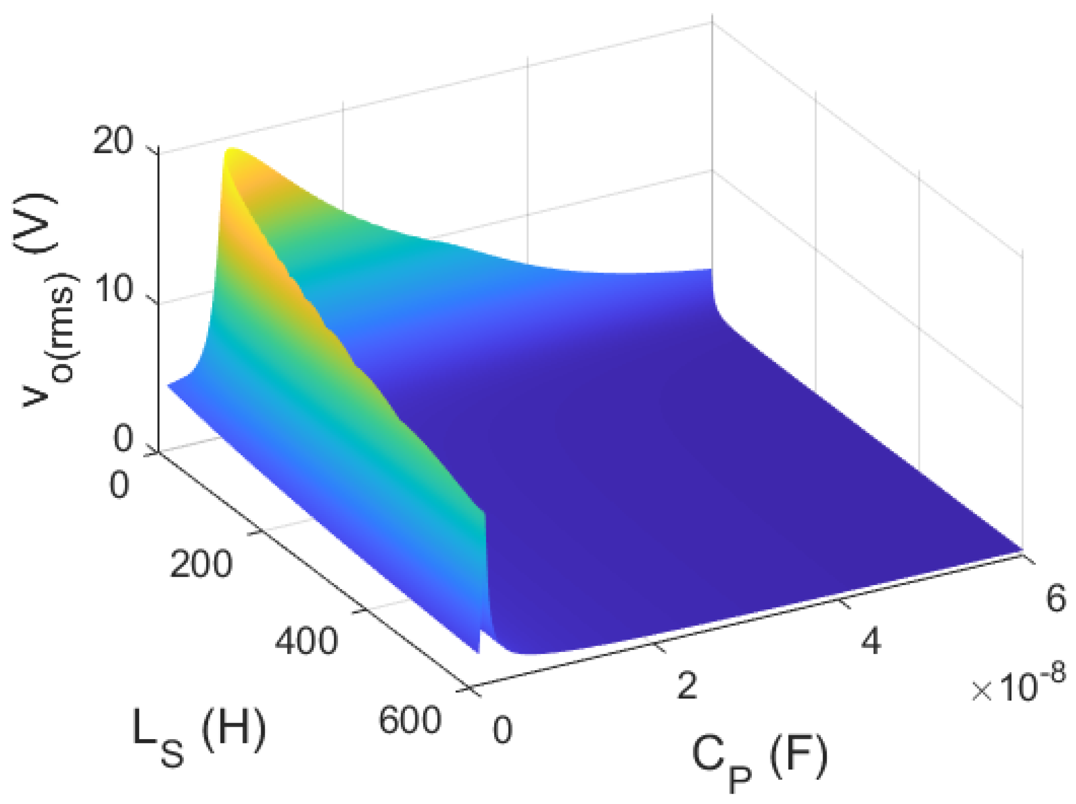
To optimize the matching network, we solved the stationary Lyapunov Equation (24) for many values of the parameters $L_S$ and $C_P$ within a given interval. Figure 3 shows the root mean square value of the output voltage $v_{o\left(\mathrm{rms}\right)}=\sqrt{\mathrm{E}\left[v_o^2\left(t\right)\right]}$ versus the values of $L_S$ and $C_P$. The values of the other parameters used in our analysis are summarized in

Table 1. Values of the energy harvester parameters.

Parameter	Value
m	1 g
$\gamma$	0.012 Ns/m
k	5.4046 · 10${}^3$ N/m
$C_{\mathrm{p}z}$	80 nF
$R_L$	1 M$\mathsf{\Omega }$
$\alpha$	0.0042 N/V (As/m)
$\epsilon$	${10}^{-3}$ (dimensionless)

, and they are well comparable to those used in several other recent works, e.g., [33,38,45]. The output voltage shows a maximum for $L_S^{\left(\mathrm{opt}\right)}=22.91$ H, and $C_P^{\left(\mathrm{opt}\right)}=8.53$ nF, with $v_{o\left(\mathrm{rms}\right)}^{\max }=20.59$ V. For comparison, the energy harvester with resistive load offers an output voltage $v_{o\left(\mathrm{rms}\right)}^{\max }=4.43$ V. The average output voltage, average output power and power efficiency for the two setups are summarized in

Table 2. Root mean square value of the output voltage, output average power and power efficiency for the energy harvester with the two different load setups.

Configuration	Voltage (rms)	Maximum Power	Efficiency
Resistive load	4.43 V	19.61 $\mathsf{\mu }$W	3.9%
Matched load	20.59 V	424.1 $\mathsf{\mu }$W	84.8%

.

The high value for the inductance in the matching network is a numerical artifact, a consequence of the relatively high value assumed for the inertial mass $m=1$ g. The inductance could be reduced considering a lighter inertial mass and of course also reducing the harvested power. An alternative solution could be the use of an active element (an inductance emulator) in the matching network that can produce high inductance values but would require an external power source. Notice that a significant increment of the harvested power can be obtained even using a sub-optimal value of the inductance. Finally, it is well known that piezoelectric transducers require high inductance values for shunting and matching. The realization of large inductances is an important research topic, and very promising results have recently been obtained, see, for example, [46].

6. Nonlinear System Analysis

When the inertial magnetic mass and the tip magnet are close enough, magnetic repulsion induces bi-stability, forcing the beam to the left or to the right of the vertical position. The magnetic force makes two vertically tilted positions stable equilibrium points, associated to the local minima of the potential energy, while the vertical position becomes an unstable equilibrium associated to a local potential energy maximum. For ambient mechanical vibrations of small amplitude, the beam is expected to oscillate around one of the two equilibria, remaining confined within the corresponding potential well. If the vibration intensity is large enough, however, fluctuations of the beam around the resting position are combined with random jumps from one well to the other. As the noise intensity becomes large enough, the beam will exhibit more frequent excursions between the two wells, with a motion ultimately resembling a random wandering around the vertical position.

To account for such bi-stability, we shall assume a potential function of the form $U\left(x\right)=-k_1{x}^2/2+k_3{x}^4/4+U_0$, where $k_1$ and $k_3$ are the linear and the nonlinear elastic constants, respectively, and $U_0=k_1^2/\left(4k_3\right)$. Using the diagonal matrix (17), the following SDEs system is obtained:

$$d{\mathbf{X}}_t=\left({\mathbf{A}}_0{\mathbf{X}}_t+\mathbf{n}\left({\mathbf{X}}_t\right)\right)dt+\epsilon \mathbf{B}d{W}_t$$

(25)

where

$${\mathbf{A}}_0=\left[\begin{array}{ccccc}0& 1& 0& 0& 0\\ 1& -\rho & -\beta & 0& 0\\ 0& \alpha & 0& -1& 0\\ 0& 0& \mu & 0& -\mu \\ 0& 0& 0& \eta & -\delta \end{array}\right],\mathbf{B}={[0,\sigma ,0,0,0]}^T$$

(26)

and $\mathbf{n}\left(x\right)={[0,-\kappa x^3,0,0,0]}^T$, with $\kappa =k_3/k_1$.

Proceeding in full analogy with the linear case, the evaluation of the output average power corresponds to the calculation of the second-order moments. However, differently from the linear case, for a generic nonlinear systems, it is impossible to derive closed equations for the moments. In fact, because of the nonlinear term in (25), the ODEs system for $\mathrm{E}\left[{\mathbf{X}}_t^n\right]$ will include terms such as $\mathrm{E}\left[{\mathbf{X}}_t^{n+2}\right]$ for all $n=1,2,\dots$, thus leading to an infinite hierarchy of coupled ODEs. A possible workaround is to make some a priori assumption about the probability density function for ${\mathbf{X}}_t$. Under a suitable hypothesis, it is possible to express higher-order moments as functions of the lower-order ones, a methodology termed moment closure technique [47].

A quite common choice amounts to assume that the stochastic process obeys a multivariate Gaussian distribution. In general, it is neither possible to justify such an assumption rigorously nor to prove that the approximated results converge to the exact values. However, there is a large amount of evidence that the method provides accurate enough results, especially if the system is subject to weak white Gaussian noise and is characterized by underlying deterministic dynamics exhibiting a stable solution [47].

We proceed as follows:

• We assume ${\mathbf{X}}_t\sim \mathcal{N}(\mu ,\sigma )$, and we derive the ODEs system for the first two order moments. All higher order moments in the ODE system are expressed as functions of the first and second order moments.
• We solve the moment ODEs system in the weak noise limit, for all values of the matching network parameters $L_S$ and $C_P$ in a given interval, finding the optimal values that maximize the output average power and power efficiency.
• In the strong noise limit, we solve the full SDEs system numerically, using the values of $L_S$ and $C_P$ determined in the previous step, to verify whether the matched load offers better performance in terms of output average power and power efficiency with respect to the resistive load setup.

To begin with, we introduce the centered variable ${\overline{\mathbf{X}}}_t={\mathbf{X}}_t-\mu$. Then, ${\overline{\mathbf{X}}}_t\sim \mathcal{N}(0,\overline{\sigma })$, where $\overline{\sigma }=\mathrm{E}\left[{\overline{\mathbf{X}}}_t{\overline{\mathbf{X}}}_t^T\right]$ is the covariance matrix, and

$$d{\overline{\mathbf{X}}}_t=\left({\mathbf{A}}_0({\overline{\mathbf{X}}}_t+\mu )+\mathbf{n}({\overline{\mathbf{X}}}_t+\mu )\right)dt+\epsilon \mathbf{B}d{W}_t$$

(27)

By definition, asymptotically ${\overline{\mathbf{X}}}_t\to 0$ for $t\to +\infty$, and therefore, taking expectations, $\mu$ solves

$${\mathbf{A}}_0\mu +\mathrm{E}\left[\mathbf{n}({\overline{\mathbf{X}}}_t+\mu )\right]=0$$

(28)

For a multivariate centered normal distribution, k-th order central moments are null if k is odd, while even orders can be expressed in terms of the elements of the covariance matrix. In particular,

$$\mathrm{E}\left[{({\overline{X}}_1+{\mu }_1)}^3\right]=3{\mu }_1{\overline{\sigma }}_{11}+{\mu }_1^3$$

(29)

and using the definition of $\mathbf{n}({\overline{\mathbf{X}}}_t+\mu )$, we have

$$\mathrm{E}\left[\mathbf{n}({\overline{\mathbf{X}}}_t+\mu )\right]=-\kappa {\mu }_1\left[\begin{array}{c}0\\ {\mu }_1^2+3{\overline{\sigma }}_{11}\\ 0\\ ⋮\\ 0\end{array}\right]$$

(30)

For the second-order central moment, repeating the steps (22) and (23), we obtain the nonlinear Lyapunov equation

$${\displaystyle \frac{d\overline{\sigma }}{dt}}={\mathbf{A}}_0\overline{\sigma }+\overline{\sigma }{\mathbf{A}}_0^T+\mathrm{E}\left[\mathbf{n}({\overline{\mathbf{X}}}_t+\mu ){\overline{\mathbf{X}}}_t^T\right]+\mathrm{E}\left[{\mathbf{X}}_t{\mathbf{n}}^T({\overline{\mathbf{X}}}_t+\mu )\right]+{\epsilon }^2\mathbf{B}{\mathbf{B}}^T$$

(31)

A straightforward calculation yields

$$\mathbf{n}({\overline{\mathbf{X}}}_t+\mu ){\mathbf{X}}_t^T=-\kappa \left[\begin{array}{cccc}0& 0& \dots & 0\\ {({\overline{X}}_1+{\mu }_1)}^3{\overline{X}}_1& {({\overline{X}}_1+{\mu }_1)}^3{\overline{X}}_2& \dots & {({\overline{X}}_1+{\mu }_1)}^3{\overline{X}}_n\\ 0& 0& \dots & 0\\ ⋮& ⋮& \ddots & ⋮\\ 0& 0& \dots & 0\end{array}\right]$$

(32)

For a multivariate centered normal distribution,

$$\begin{array}{cc}\hfill \mathrm{E}\left[{({\overline{X}}_1+{\mu }_1)}^3{\overline{X}}_1\right]& =3{\overline{\sigma }}_{11}\left({\overline{\sigma }}_{11}+{\mu }_1^2\right)\hfill \end{array}$$

(33a)

$$\begin{array}{cc}\hfill \mathrm{E}\left[{({\overline{X}}_1+{\mu }_1)}^3{\overline{X}}_j\right]& =3{\overline{\sigma }}_{1j}\left({\overline{\sigma }}_{11}+{\mu }_1^2\right)\hfill \end{array}$$

(33b)

and therefore,

$$\begin{array}{cc}\hfill & \mathrm{E}\left[\mathbf{n}({\overline{\mathbf{X}}}_t+\mu ){\mathbf{X}}_t^T\right]+\mathrm{E}\left[{\mathbf{X}}_t{\mathbf{n}}^T({\overline{\mathbf{X}}}_t+\mu )\right]=\hfill \\ \hfill & \hspace{1em}\hspace{1em}-3\kappa \left({\overline{\sigma }}_{11}+{\mu }_1^2\right)\left[\begin{array}{ccccc}0& {\overline{\sigma }}_{11}& 0& \cdots & 0\\ {\overline{\sigma }}_{11}& 2{\overline{\sigma }}_{12}& {\overline{\sigma }}_{13}& \cdots & {\overline{\sigma }}_{1n}\\ 0& {\overline{\sigma }}_{13}& 0& \cdots & 0\\ ⋮& ⋮& ⋮& \ddots & ⋮\\ 0& {\overline{\sigma }}_{1n}& 0& \cdots & 0\end{array}\right]\hfill \end{array}$$

(34)

Substituting (30) and (34) into (28) and (31), respectively, we obtain a system of nonlinear differential algebraic equations (DAEs) that can be solved numerically to determine the admissible values for $\mu$ and $\overline{\sigma }$, from which the covariance matrix $\sigma$ is readily derived.

Figure 4 shows the root mean square output voltage for the nonlinear bistable energy harvester, as a function of the matching network parameters $L_S$ and $C_P$. The elastic constant model parameters are set to the values $k_1=5.4046$ kN/m and $k_3=5.4046$ TN/m. The latter is chosen to be very large to achieve a reasonably small value for the displacement x. The other parameters are the same as those of Table 1. The output voltage achieves the maximum value of $v_{o\left(\mathrm{rms}\right)}^{\max }=20.59$ V for $L_S^{\left(\mathrm{opt}\right)}=11.6$ H and $C_P^{\left(\mathrm{opt}\right)}=8.63$ nF. Interestingly, the optimal inductance value is a little lower for the nonlinear system with respect to the linear case. Note that since the noise intensity is very small, the figure resembles that of the linear system. However, since the equilibrium position is not the vertical resting state, the optimal values of the parameters are different.

Figure 5 shows the root mean square output voltage as a function of the noise intensity. Red squares refer to the energy harvester with matched load with optimal values of the circuit components given above. Blue circles refer to the energy harvester with a simple resistive load. The output voltage was obtained from the numerical integration of the SDEs system using the stochastic Runge–Kutta method. For each value of the noise intensity, we averaged over 20 simulations, each one with a different realization of the noise process, with time length $\mathsf{\Delta }T={10}^4$ s and time integration step $\delta t\approx 50$ $\mathsf{\mu }$s. Root mean square values were calculated averaging over all simulations, after removing the initial transients. We notice that although the matching network optimization is carried out for a small noise intensity, the matched load setup offers higher output voltage, and therefore higher output average power and better power efficiency, also for a relatively high noise intensity. 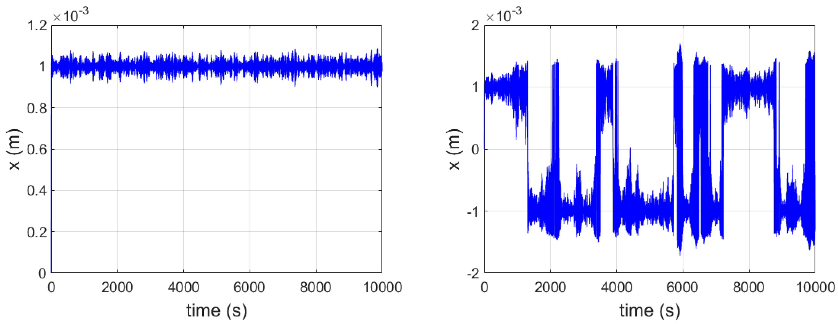Figure 6 shows the displacement x versus time for two values of the noise intensity. On the left, for $\epsilon ={10}^{-3}$, the beam–inertial mass system remains confined in the right potential well, vibrating around the equilibrium position with small amplitude. On the right, for $\epsilon =5·{10}^{-3}$, the beam–inertial mass system jumps irregularly back and forth from one well to the other. In all our simulations, the initial condition was set to $\mathbf{X}\left(0\right)=0$, with the beam–mass system falling in the left or in the right potential well depending on the initial value of the Wiener process.

To validate the accuracy of the method based on Gaussian moment closure, we compare theoretical predictions with results from numerical simulations. Figure 7 shows the relative error between theoretical predictions obtained using the Gaussian moment closure method and numerical simulations changing the noise intensity, for both the root mean square output voltage (red squares) and the power efficiency (blue circles). The relative error is evaluated as

$$\mathsf{\Delta }x=\left|{\displaystyle \frac{x_{\mathrm{theoretical}}-x_{\mathrm{numerical}}}{x_{\mathrm{numerical}}}}\right|$$

(35)

As expected, the relative error is very small for weak noise, and it increases along with the noise intensity. The error becomes rapidly significant when the beam begins to jump between the two potential wells because the corresponding probability density function is no longer a multivariate Gaussian.

7. Conclusions

Ambient dispersed energy is a potentially unlimited energy source that can be exploited for supplying power to the next generation of wireless connected IoT electronic devices. In particular, parasitic mechanical vibrations are very promising for their relatively high power density and they widespread presence.

In this work, we studied a bi-stable piezoelectric energy harvester for parasitic ambient mechanical vibrations scavenging. We showed that the application of matching network, interposed between the piezoelectric transducer and the electrical load, increases the harvested power and the power conversion efficiency by more than 30 times in the weak noise limit, and by more than five times for medium–strong noise intensity.

The matching network is designed to reduce the impedance mismatch between the mechanical and the electrical domains of the harvester. With respect to other previously proposed solutions based on power factor correction, the new setup not only reduces the reactive power reflected by the load to the source but also maximizes the average power absorbed by the load.

To properly optimize the matching network, we developed a novel design methodology. For a linear harvester, the optimal values of the matching network elements can be determined analytically applying stochastic analysis methods and solving the resulting Lyapunov equation. For a nonlinear harvester, we developed a technique based on finding an approximate solution for a nonlinear Lyapunov equation applying the Gaussian moment closure method. The proposed methodology represents a significant improvement for the design of nonlinear systems, for which few techniques are currently available.

Although the design methodology is best suited for weak noise intensity, we verified through numerical simulations that the application of the optimized matching network offers a significant boost in the power performance of the energy harvester, even for the medium–high intensity of ambient mechanical vibrations.