A Study of Wind Shear Influences on the Aerodynamic Performances of a UAV Airfoil

Featured Application

This paper investigates the aerodynamic performances of a UAVs airfoil in different shear wind environments, and the results will provide guidance for flight attitude control and flight trajectory selection in different shear winds, especially for long-range flight with very low energy consumption of bionic UAVs using shear wind field energy.

Abstract

In order to study the flight strategies of birds in shear wind and realize the long-range flight of an unmanned aerial vehicle (UAV), the aerodynamic performances of a UAV’s airfoil under different shear wind are studied using numerical methods. The results are calculated using the RANS method in shear wind with a linear and logarithmic distribution of velocity. The results show that the slope of the lift curve, the maximum lift coefficient and the stall angle decrease when the velocity gradient is positive or increasing, conversely, they increase at a negative gradient compared to gradient-free wind fields. A positive gradient of wind significantly increased the maximum lift-drag ratio and the effective angle of attack. Compared with linear distributed shear wind with the same velocity at both the lowest and highest points of the flow field, logarithmic distribution decreases the slope of the lift curve, the maximum lift coefficient and the maximum lift-drag ratio and the effective angle of attack. Therefore, a shear wind with a positive gradient is beneficial to the increase of lift-drag ratio and more conducive to cruise flight, and a negative gradient is beneficial for increased lift and more conducive to take-off and landing of UAVs. The velocity distributions influence the aerodynamic performances of the airfoil which is related to the speed and gradient distribution of shear wind.

1. Introduction

Shear wind is a very common flow in the atmosphere [1] resulting in the temporal or spatial variability of wind. In 1983, the National Research Council (NRC) gave a more specific definition of shear wind as wind speed at two points in space divided by the distance between two points [2]. For aircraft flight and mechanical operation, shear wind is generally considered to be a critical factor. For example, shear wind can reduce the generated power of large wind turbines [3] but increase wind turbine blade loads [4]. Shear wind also affects civil aviation aircraft, with rapidly changing airspeeds in a low-altitude shear wind causing sudden changes in aircraft lift and manoeuvrability, resulting in aircraft deflection from the intended trajectory or even flight accidents [5,6,7]. Aiming at reducing flight accidents, NASA has proposed an F-factor capable of assessing the degree of shear wind hazard from a flight mechanics perspective [8]. In addition, shear wind also has an impact on the flight and control of long-range shell rockets, which can easily cause flight deviation and the reduction of flight stability [9,10]. Therefore, for conventional aircraft and fluid machinery, how to reduce the effects of shear wind is an important research topic to ensure flight safety and maintain operational efficiency. However, for birds in nature, shear wind is a common flow pattern.

In nature, many birds have the ability to use wind field energy to achieve long-distance flight. For example, frigate birds and albatrosses use shear wind and updrafts [11] to achieve long-distance gliding flight with very low energy consumption by harnessing the energy of the wind field. The king of flight-albatross can traverse strong wind gradients near the sea surface [12] and climbs and glides down at high and low altitudes in shear wind fields. During the flight, they obtain frontal energy and offset drag consumption to achieve long-range flight [13].

Nowadays, the flight range of UAVs is constrained by power supply, and flight time and range are greatly limited. Studies have shown that there are two ways to extend UAV flight range. First, the endurance performance of a UAV can be improved by optimizing the aerodynamic layout and drag reduction design. However, the efficiency is limited. In the second, a UAV can use wind energy through flight attitude adjustment with the help of wind field flow. In this manner, its own energy consumption can be significantly reduced to achieve long-range flight. Therefore, according to the flight mode of albatrosses in shear wind, people have carried out studies on UAV trajectory planning [14], flight strategies [15] and dynamic glide monitoring [16] in shear wind. Flight trajectory optimization [17,18,19,20] and flight attitude adjustment [21] in shear wind have been examined to achieve low-energy flight.

However, the flight performance of a man-made glider controlled by a dynamic model is much less [22,23] than that of the albatross. Imitating the flight attitude and trajectory of birds cannot achieve low-energy flight to achieve long-range flight, and analysis of aerodynamic performance under a flow field environment should be carefully performed to achieve excellent performances.

Therefore, according to the safety and efficiency requirements of UAV flight, utilizing the shear wind energy during flying just like a bird can be a good bionic inspiration, which is considered to be favorable for UAV design. The shear wind effect on the aerodynamic performance of a UAV’s airfoil is studied by numerical simulation. A series of shear winds are generated, and the impact of shear wind velocity distribution on aircraft flight performance is investigated. Lift enhancement, drag reduction and range increase are the expected result for UAV flight. How to perform flight control from the perspective of aerodynamics in shear wind is studied in the current research. Therefore, in this paper, it is estimated that the findings can be a guide for long-range flight with low energy consumption.

2. Numerical Simulation Model and Shear Wind Model

2.1. Numerical Model

As an important aerodynamic component of UAVs, the aerodynamic distribution of the wing is of great significance to an aircraft. The findings of the current investigation are intended to lay fundamental research for the design and flight attitude control of a small UAV. The drone has been designed with a wingspan of two meters, and a maximum flight speed of 100 m/s. A symmetrical wing airfoil NACA0012 is chosen for the drone.

In this paper, we study the effect of shear wind on the aerodynamic performances of a two-dimensional NACA0012 airfoil with a chord length of 0.573 m using ANSYS Fluent software. In the numerical calculations, the finite volume method is used to discretize Navier-Stokes equations, a second-order windward format is used for spatial discretization, and a k-ω SST turbulence model [24] is selected. A 15-times chord length is used for the far field in the computational domain. A C-H type structure grid with a size of 715 × 201 is generated, and the first layer grid height is generated according to the law of y+ = 1. Details of the grid are shown in Figure 1.

2.2. Shear Wind Model

Numerous velocity distributions usually appear in a natural shear wind, which has a great influence on UAV performances. In this paper, three different wind profiles, gradient-free wind, linear distributed shear wind and logarithmic distribution shear wind are selected to study these influences. The three wind profiles are defined as follows:

Gradient-free wind: The wind field without gradient is defined in the gradient-free wind model, which is defined in Equation (1).

$$V_{\mathrm{W}}=C$$

(1)

In Equation (1), V_W is the wind speed at height h, which is selected as Mach number 0.3, Mach number Ma = V_W/a, and a is sound speed. The Mach number corresponding to C in this paper is 0.3. As shown in Figure 2, the velocity has no gradient along the height direction and wind speed is constant.

Linear distributed shear wind: The velocity magnitude varies linearly along the height direction while the wind direction remains the same. The velocity profile against height is defined in Equation (2), i.e., dV_W/dh is constant. Schematic diagrams of the shear wind field with positive and negative gradients are shown in Figure 3.

$$V_{\mathrm{W}}=V_{\mathrm{W}hmin}+\left(\frac{V_{\mathrm{W}hmax}-V_{\mathrm{W}hmin}}{h_{max}-h_{min}}\right)(h-h_{min})$$

(2)

where h_min and h_max are heights at the lowest and highest positions in the wind field, V_Whmin and V_Whmax are the corresponding velocities. It is shown that velocity gradient with dV_W/dh = ±3.05, 2.29 and 1.52 are used for the four wind profiles, while the Mach number M = 0.3 is set for wind speed, as listed in

Table 1. Parameters of four wind models.

Ma_VWhmin	Ma_VWhmax	dVW/dh	Ma_VWhavg
0.2	0.4	3.05	0.3
0.4	0.2	−3.05	0.3
0.225	0.375	2.29	0.3
0.25	0.35	1.52	0.3

. A positive and negative gradient velocity gradient is characterized using the dV_W/dh, and dV_W/dh = −3.05 is used for the negative one.

Logarithmic distribution shear wind: A logarithmically distributed shear wind profile is established using the experimental wind data proposed by Ricardo Bencatel [25]. The observed wind data is fitted and estimated using a particle filtering approach to establish the mathematical model, as defined in Equation (3).

$$\begin{gathered} V_{\mathrm{W}}=V_{\mathrm{W}hmin}+\frac{∆V_{\mathrm{W}h}}{2}[1+\mathrm{erf}(4\frac{h-h_{avg}}{h_{max}-h_{min}})] \\ ∆V_{\mathrm{W}h}={V_{\mathrm{W}hmax}-V}_{\mathrm{W}hmin} \\ {h}_{avg}=(h_{max}+h_{min})/2 \end{gathered}$$

(3)

where erf is the error function; ΔV_Wh is the velocity difference within the wind field, ΔV_Wh = V_Whmax − V_Whmin; h_avg represents the average height of the wind field, h_avg = (h_max + h_min)/2. The Mach numbers corresponding to V_Whmin and V_Whmax are 0.2 and 0.4, respectively. A typical velocity profile is shown in Figure 4.

3. Results and Discussion

3.1. Numerical Method Validation

In order to verify the numerical method, numerical simulation of the NACA0012 airfoil is performed at a freestream condition with Mach number Ma = 0.3 and Reynolds number Re = 4.0 × 10⁶. It should be noted that grid independence has been verified. The grid mesh size and distribution are carefully adjusted to ensure the numerical results are no longer changed due to the change of the grid. Because NACA0012 is a very common benchmark which has been discussed in many studies, grid independence will not be discussed in this paper. As a result, the numerical calculation results are consistent with the experimental results as shown in Figure 5. Compared with experimental results [26], the results show that the lift curve and airfoil surface pressure are in good agreement with experimental results in the literature. Therefore, the numerical simulation method and calculation grid of this paper meet the calculation requirements, the results of subsequent numerical calculations in this paper are credible and the conclusions obtained are reliable.

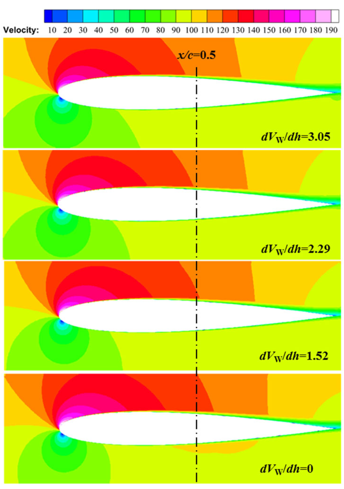
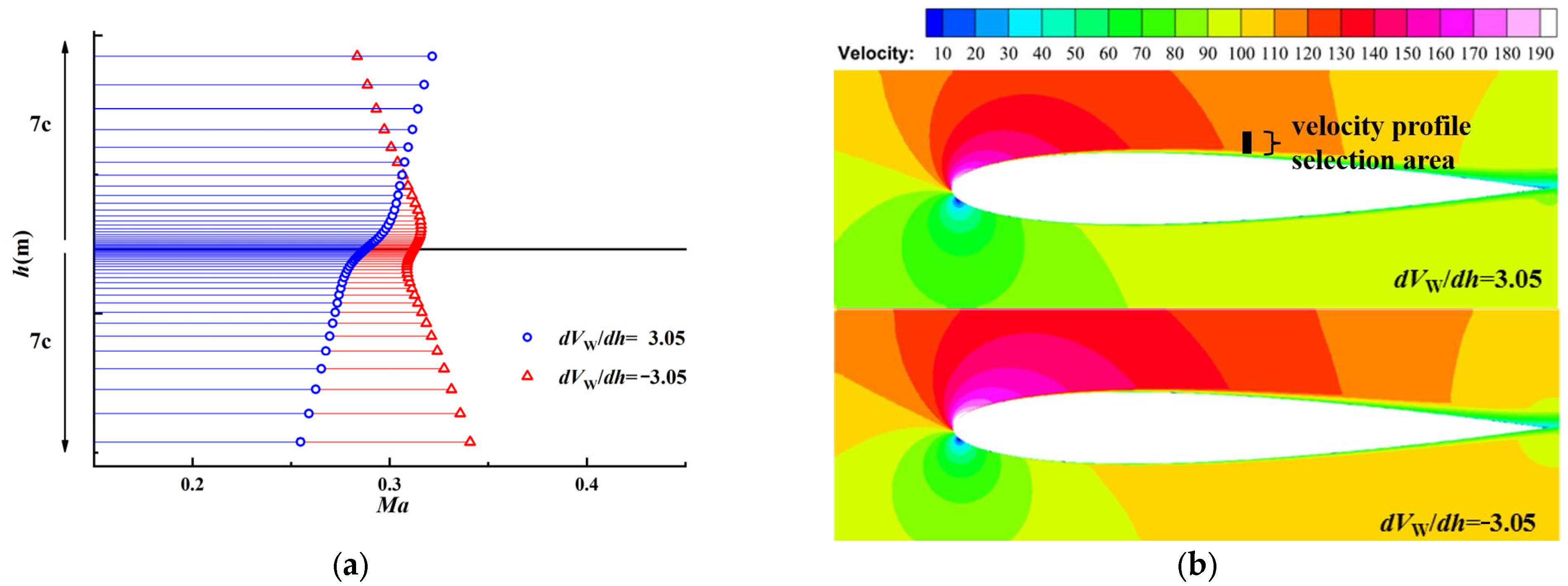
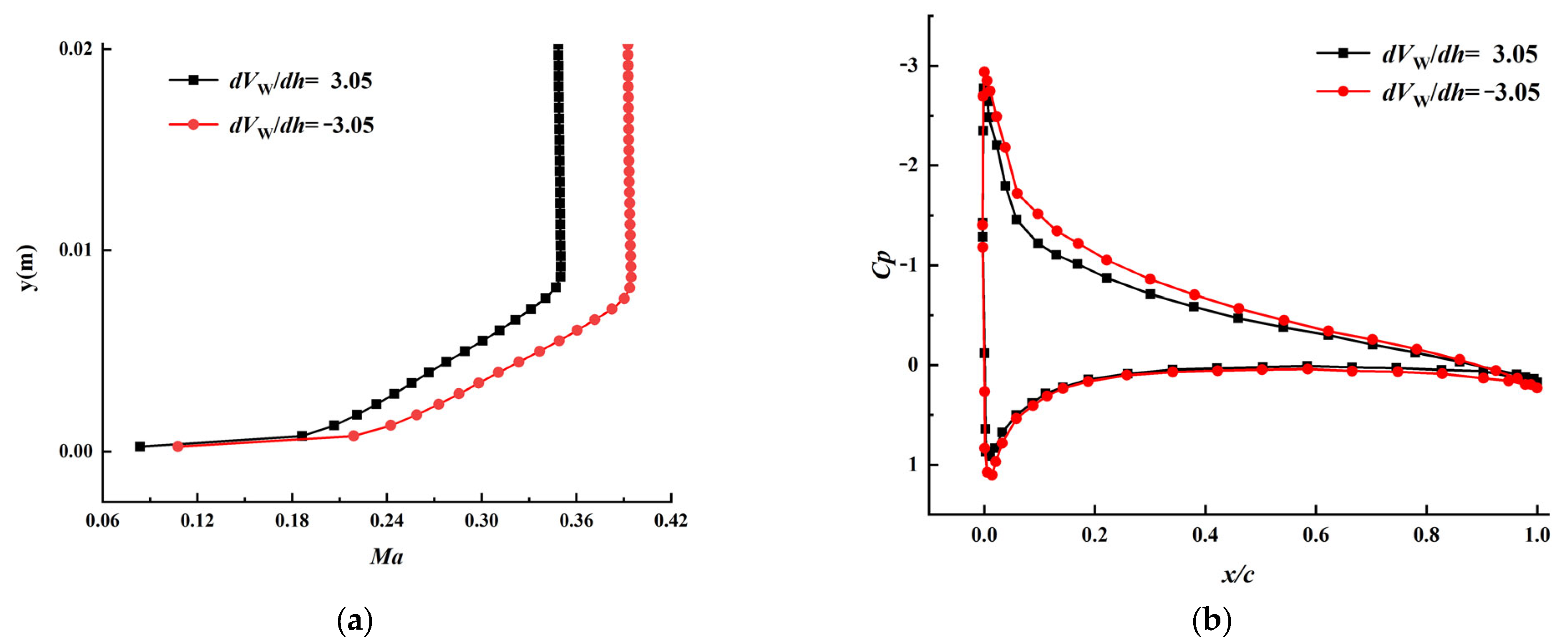
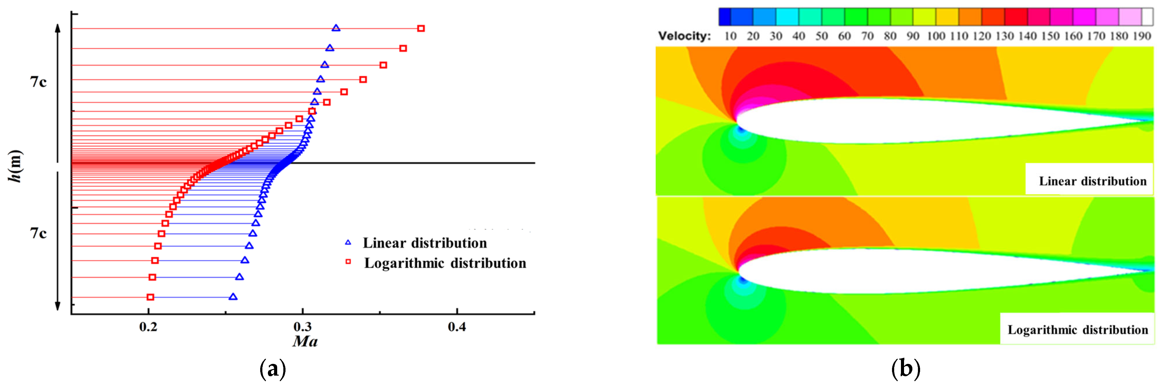
3.2. Effect on Velocity Distribution

Wind shear affects aerodynamic performance by changing the air direction flow across the airfoil. As a result, velocity distribution at the leading edge of the airfoil is changed. As seen in Figure 6a, L is the distance to the leading edge of the airfoil. When the wind velocity gradient is positive, velocity near the chord axis at L = c (c is the chord length of the airfoil) is smaller than that of the Gradient-free wind case. It is found that the surface pressure is reduced as wind velocity decreases, resulting in a lift reduction. Shear velocity near the airfoil surface and friction drag is also reduced as the wind velocity gradient near the chord axis decreases.

The velocity profile before the airfoil was under different gradients is illustrated in Figure 6b. As the airflow passes the airfoil, the rearranged velocity distributions are depicted in Figure 7. It is shown that the velocity magnitude near the chord axis decreases from 125 m/s to 118 m/s as the velocity gradient increase from 0 to 3.05. On the other hand, air velocity behind the lower airfoil surface remains almost the same in the four cases. It can be estimated that lift has decreased as the velocity gradient increased from 0 to 3.05.

Influences of negative velocity gradient are also discussed in the current research as shown in Figure 8. Wind velocity decreases with height for the negative velocity gradient case. Contrary to the positive gradient case, more large wind velocity appears near the chord axis at L = c, as shown in Figure 8a. The velocity contour around the airfoil is illustrated in Figure 8b. In order to quantitively measure the variation of the flow field, both velocity profile and pressure distribution along the airfoil upper surface are extracted as shown in Figure 9a,b. It is shown that air around the airfoil has been accelerated above the airfoil up surface due to the negative effect while the one below the lower surface remains almost the same. On the other hand, a negative gradient has decreased pressure along the upper surface but increased the one along the lower surface. This negative effect is impressively found at the airfoil leading edge resulting in an enhanced pressure suction phenomenon. Thus, the lift is estimated to be enhanced. Furthermore, surface shear stress increases against the velocity gradient which usually implies a larger frictional drag.

As shown in Figure 10, the Logarithmic distribution of shear wind, velocities at L = c ahead of the leading edge is found to be smaller than the one of the linear distributed shear wind field with dV_W/dh = 3.05. Because the velocity gradient dV_W/dh ahead of the leading edge is larger than 3.05 for the logarithmic distribution shear wind case, it results in smaller airfoil leading edge velocities and velocity gradients compared with those of linear distributions shear wind which is dV_W/dh = 3.05. The logarithmically distributed effect results in dramatically slowed down air above the upper surface which in turn leads to a decrease in lift. Similarly, the logarithmic distribution leads to a decrease in the velocity gradient near the chord axis, which in turn reduces the shear stress and frictional drag.

This section discusses shear wind fields with different velocity gradients and distributions, containing linear shear wind fields with positive velocity gradients, linear shear wind fields with negative velocity gradients, and shear wind fields with logarithmic velocity distributions. In the paper, the effects of different shear wind fields on the aerodynamic performance of the airfoil are discussed by analyzing the velocity distribution and pressure distribution near the leading edge and surface of the airfoil.

3.3. Effect of Shear Wind on Lift

Both lift and lift-drag ratios are critical for a bionic UAV design, thus the effect of shear wind on lift and lift-drag ratio is further discussed in the current research. According to the previous study on velocity and pressure distributions, both lift and drag have been estimated. The lifts of the four position cases of the linear distributed shear wind are illustrated in Figure 11a and the negative case is compared in Figure 11b. It is shown that the maximum CL has decreased as dV_W/dh increases. Compared with a wind field with zero gradient, the maximum lift coefficient was reduced by 18% in a shear wind with dV_W/dh = 3.05, 13.4% for dV_W/dh = 2.29 shear wind, and 8% for dV_W/dh = 1.52 shear wind. So, it is verified that a positive gradient reduces the maximum lift coefficient, and the greater the gradient is, the lower the maximum lift coefficients are. A positive velocity gradient also decreases the corresponding stall angle. For an aircraft, a positive gradient at the same angle of attack usually reduces lift which is not beneficial to take-off and landing which may lead to a flight accident. Therefore, a UAV needs to increase the angle of attack to maintain lift under a positive gradient shear wind situation.

The lift curve of a negative gradient case is shown in Figure 11b. It is shown that a negative gradient increases lift which is consistent with the conclusion discussed in the previous Section 3.2. Compared to a positive gradient, a negative gradient also increases the slope of the lift curve, maximum lift coefficient and stall angle of attack. Compared to a gradient-free wind, the maximum lift coefficient of the negative gradient is increased by 19.6% and the stall angle of attack is increased to 16°. Therefore, a negative gradient increases lift and delays stall at the same average speed, which is the reason why birds use shear wind to keep rising to gain potential energy and finally achieve long-distance gliding flight. Therefore, only a small angle of attack is needed to generate sufficient lift required for the ascent in a negative gradient wind, which is of great value for the take-off and landing of UAVs.

Similarly, shear wind velocity studies show that logarithmic distribution reduces lift. For the same conditions of V_Whmin, V_Whmax and V_Whavg, logarithmic distribution decreases the slope of the lift curve and maximum lift coefficient, and increases stall angle. The maximum lift coefficient is also decreased by 39.9% compared to linear distribution with dV_W/dh = 3.05, as shown in Figure 12.

3.4. Effect of Shear Wind on Lift-Drag Ratio

Based on previous velocity analysis, it can be concluded that a positive gradient of shear wind decreases lift and drag, a negative gradient increases lift and drag, and logarithmic distribution decreases lift and drag, which shows that variations of lift and drag under shear wind are consistent with each other. In order to comprehensively evaluate the effect of shear wind on airfoil lift and drag, this section seeks the optimal performance of airfoil in a shear wind field through the study of the lift-drag ratio of the airfoil. The effectiveness of an airfoil is highly dependent on the lift-drag ratio which is an important parameter of airfoil aerodynamic performance.

Figure 13a shows that the maximum lift-drag ratio of an airfoil, as well as the corresponding angle of attack, increases significantly when the velocity gradient is increased. When the gradient is reduced to dV_W/dh = 1.52, the maximum lift-drag ratio is decreased by 28.8% for the dV_W/dh = 3.05 condition. Considering decreases in lift and increases in lift-drag ratio at a positive gradient, it can be deduced that airfoil drag has been significantly reduced. Therefore, a positive gradient is more conducive to the cruising flight of a vehicle, which is the reason why birds can cruise long distances in shear wind fields with very little energy consumption. If aircraft could adopt air energy in shear winds, they will achieve long-distance flight with very low energy consumption.

A negative gradient will significantly reduce the maximum lift-drag ratio of the airfoil and its corresponding angle of attack. As a result, the maximum lift-drag ratio is lower than the one of the gradient-free case, and the corresponding angle of attack is shifted forward, as shown in Figure 13b. Considering the increased lift, increased drag and decreased lift-drag ratio, it can be deduced that the drag has been significantly increased due to the negative gradient effect. Thus, a negative gradient effect is not conducive to the cruise flight of aircraft. On the contrary, it is beneficial for landing and reducing glide distance as larger lift and drag are both required in the flight situation. The logarithmic distribution of shear wind will also reduce the lift, drag and lift-drag ratio as shown in Figure 14. The maximum lift-drag ratio and the corresponding angle of attack are slightly decreased compared with those of the gradient-free case.

4. Conclusions

Shear wind has great influences on the aerodynamic performances of a UAV, and the effect of shear wind on the velocity distributions, lifts and lift-drag ratios are investigated. In this paper, we evaluate that:

• Three wind shear models are established to present a comparative analysis of the altitude impact on velocity. Shear wind velocity gradient has a significant influence on both velocity profile and velocity gradient which affects pressure and fluctuating velocity distribution around the airfoil. A positive gradient reduces velocities near the airfoil leading edge, but a negative gradient increases them. On the other hand, a positive gradient and logarithmic distribution will reduce the lift curve slope, the maximum lift coefficient and the stall angle of attack. Conversely, a negative gradient will increase the slope of the lift curve, maximum lift coefficient, and stall angle of attack.
• A positive gradient of shear wind increases the maximum lift-drag ratio and its corresponding angle of attack. Therefore, a UAV can obtain a larger lift-drag ratio when suffering a positive gradient shear wind. On the contrary, high lift and high drag can be achieved for the negative gradient case which can greatly reduce the take-off and landing distance of the UAV. The vertical take-off and landing capability is expected to be realized through the comprehensive optimization design of the UAV.

The findings in the current research can be used for the UAV design to achieve long-range flight and they provide a foundation for further experimental and computational studies on bird flight with low energy consumption.

References

1. Bencatel, R.; Sousa, T.J.D.; Girard, A. Atmospheric Flow Field Models Applicable for Aircraft Endurance Extension. Prog. Aerosp. Sci. 2013, 61, 1–25. [Google Scholar] [CrossRef] [Green Version]
2. Federal Aviation Administration. Windshear Training Aid, Example Training Program; Federal Aviation Administration: Washington, DC, USA, 1986.
3. Kavari, G.; Tahani, M.; Mirhosseini, M. Wind shear effect on aerodynamic performance and energy production of horizontal axis wind turbines with developing blade element momentum theory. J. Clean. Prod. 2019, 219, 368–376. [Google Scholar] [CrossRef]
4. Chun, C.; Chiang, P. Turbulence effects on the wake flow and power production of a horizontal-axis wind turbine. J. Wind. Eng. Ind. Aerodyn. 2014, 124, 82–89. [Google Scholar]
5. Keohan, C. Ground-based wind shear detection systems have become vital to safe operations. ICAO J. 2007, 62, 16–19, 33–34. [Google Scholar]
6. Eggers, A.J., Jr.; Digumarthi, R.; Chaney, K. Wind Shear and Turbulence Effects on Rotor Fatigue and Load Control. J. Sol. Energy Eng. 2003, 125, 402–409. [Google Scholar] [CrossRef]
7. Roland, J. White Effect of wind shear on airspeed during airplane landing approach. J. Aircr. 1992, 29, 237–242. [Google Scholar]
8. Proctor, F.H. The Terminal Area Simulation System, Vol. I: Theoretical Formulation; NASA CR-4046, DOT/FAA/PM-86/50,I; NASA: Washington, DC, USA, 1987. [Google Scholar]
9. Wuh, Z.; Songw, D.; Zhang, L. Low level wind model building and its influence on trajectory characteristic of projectiles. J. Ordance Eng. Coll. 2015, 27, 38–42. [Google Scholar]
10. Gao, T.C.; Tu, X.W.; Fang, H.X.; Niu, Z.C. Three dimensional numerical analysis about influences of atmospheric wind field on ballistic trajectory. J. PLA Univ. Sci. Technol. Nat. Sci. Ed. 2011, 12, 178–183. [Google Scholar]
11. Pennycuick, C.J. The Concept of Energy Height i Animal Locomotion: Separating Mechanics from Physiology. J. Theor. Biol. 2003, 224, 189–203. [Google Scholar] [CrossRef] [PubMed]
12. Richardson, P.L. How Do Albatrosses Fly Around the World without Flapping their Wings? Prog. Oceanogr. 2011, 88, 46–58. [Google Scholar] [CrossRef] [Green Version]
13. Sachs, G. Minimum Shear Wind Strength Required for Dynamic Soaring of Albatrosses. IBIS 2005, 147, 1–10. [Google Scholar] [CrossRef]
14. Zhao, Y.J. Optimal Patterns of Glider Dynamic Soaring. Optim. Control Appl. Methods 2004, 25, 67–89. [Google Scholar] [CrossRef]
15. Deittert, M.; Richards, A.; Toomer, C.A.; Pipe, A. Engineless Unmanned Aerial Vehicle Propulsion by Dynamic Soaring. J. Guid. Control Dyn. 2009, 32, 1446–1457. [Google Scholar] [CrossRef]
16. Kaushik, H.; Mohan, R.; Prakash, K.A. Utilization of Wind Shear for Powering Unmanned Aerial Vehicles in Surveillance Application: A Numerical Optimization Study. Energy Procedia 2016, 90, 349–359. [Google Scholar] [CrossRef]
17. Bonnin, V.; Benard, E.; Moschetta, J.M.; Toomer, C.A. Energy-Harvesting Mechanisms for UAV Flight by Dynamic Soaring. Int. J. Micro Air Veh. 2015, 7, 213–229. [Google Scholar] [CrossRef]
18. Silva, W.; Frew, E.W. Experimental Assessment of Online Dynamic Soaring Optimization for Small Unmanned Aircraft. In Proceedings of the AIAA Infotech @ Aerospace, San Diego, CA, USA, 4–8 January 2016. [Google Scholar]
19. Shaw-Cortez, W.E.; Frew, E. Efficient Trajectory Development for Small Unmanned Aircraft Dynamic Soaring Applications. J. Guid. Control Dyn. 2015, 38, 519–523. [Google Scholar] [CrossRef]
20. Gao, C.; Liu, H.H.T. Dubins Path-Based Dynamic Soaring Trajectory Planning and Tracking Control in a Gradient Wind Field. Optim. Control. Appl. Methods 2016, 38, 147–166. [Google Scholar] [CrossRef]
21. Gao, C.; Liu, H.H.T. Dynamic Soaring Surveillance in a Gradient Wind Field. In Proceedings of the AIAA Guidance, Navigation, and Control Conference, Boston, MA, USA, 19–22 August 2013; pp. 2013–4863. [Google Scholar]
22. Lissaman, P. Wind energy extraction by birds and flight vehicles. In Proceedings of the 43rd AIAA Aerospace Sciences Meeting and Exhibit, Reno, NV, USA, 10–13 January 2005. [Google Scholar]
23. Bower, G.C. Boundary Layer Dynamic Soaring for Autonomous Aircraft Design and Validation; Stanford University: Stanford, CA, USA, 2011. [Google Scholar]
24. Scheuerer, M.; Heitsch, M.; Menter, F.; Egorov, Y.; Toth, I.; Bestion, D.; Pigny, S.; Paillere, H.; Martin, A.; Boucker, M.; et al. Evaluation of Computational Fluid Dynamic Methods for Reactor Safety Analysis (ECORA). Nucl. Eng. Des. 2005, 235, 359–368. [Google Scholar] [CrossRef]
25. Bencatel, R.; Sousa, J.; Faied, M.; Girard, A. Shear wind estimation. In Proceedings of the AIAA Guidance, Navigation, and Control Conference, Portland, OR, USA, 8–11 August 2011. [Google Scholar]
26. Dindar, M.; Kaynak, U. Effect of Turbulence Modeling on Dynamic Stall of A NACA0012 Airfoil. In Proceedings of the Aerospace Sciences Meeting and Exhibit, Reno, NV, USA, 6–9 January 1992. [Google Scholar]
Figure 1. NACA0012 airfoil grid.
Applsci 13 03764 g001
Figure 2. Schematic diagram of gradient-free wind.
Applsci 13 03764 g002
Figure 3. Schematic diagram of Linear distributed shear wind: (a) Positive gradient; (b) Negative gradient.
Applsci 13 03764 g003
Figure 4. Schematic diagram of logarithmically distributed shear wind.
Applsci 13 03764 g004
Figure 5. Aerodynamic distribution of NACA0012 (Ma = 0.3, Re = 4.0 × 10⁶): (a) Lift curve; (b) Airfoil surface pressure distribution (α = 13.5°).
Applsci 13 03764 g005
Figure 6. Velocity distribution near the chord axis in Linear distributed shear wind (L = c, α = 7°): (a) At a positive gradient and no gradient state; (b) At a different positive gradient state.
Applsci 13 03764 g006
Figure 7. Velocity magnitude contour near the airfoil surface (α = 7°).
Applsci 13 03764 g007
Figure 8. Velocity distribution of linear distributed shear wind field: (a) Velocity distribution near chord axis (L = c, α = 7°); (b) Velocity magnitude contour near the airfoil surface (α = 7°).
Applsci 13 03764 g008
Figure 9. Velocity profile and pressure distribution around airfoil surface (α = 7°): (a) Velocity profile of upper surface (x/c = 0.5); (b) Pressure distribution.
Applsci 13 03764 g009
Figure 10. Velocity distribution of logarithmically distributed shear wind field: (a) Velocity distribution near chord axis (L = c, α = 7°); (b) Velocity magnitude contour near the airfoil surface (α = 7°).
Applsci 13 03764 g010
Figure 11. Lift curve with linear wind gradient: (a) Positive gradient; (b) Negative gradient.
Applsci 13 03764 g011
Figure 12. Lift curves of the airfoil under a linear and logarithmic distribution of shear winds.
Applsci 13 03764 g012
Figure 13. The lift-drag ratio of an airfoil in Linear distributed shear wind: (a) Positive gradients; (b) Positive gradient versus negative gradient.
Applsci 13 03764 g013
Figure 14. Lift-drag ratio of airfoil with different velocity distribution of shear wind.
Applsci 13 03764 g014